Revisiting the differential freezing nucleus spectra derived from drop-freezing experiments: methods of calculation, applications, and confidence ...
←
→
Page content transcription
If your browser does not render page correctly, please read the page content below
Atmos. Meas. Tech., 12, 1219–1231, 2019
https://doi.org/10.5194/amt-12-1219-2019
© Author(s) 2019. This work is distributed under
the Creative Commons Attribution 4.0 License.

Revisiting the differential freezing nucleus spectra
derived from drop-freezing experiments: methods
of calculation, applications, and confidence limits
Gabor Vali
Department of Atmospheric Science, University of Wyoming, Laramie, Wyoming, USA

Correspondence: Gabor Vali (vali@uwyo.edu)

Received: 13 September 2018 – Discussion started: 14 November 2018
Revised: 3 February 2019 – Accepted: 6 February 2019 – Published: 26 February 2019

Abstract. The differential nucleus concentration defined in                widely used already because of its direct connection to the
Vali (1971) is re-examined and methods are given for its ap-               readily obtained frozen fraction. These functions were orig-
plication. The purpose of this document is to facilitate the               inally defined in Vali (1971; V71) and their link to different
use of differential spectra in describing the results of drop              forms, namely the differential and integral site density func-
freezing, or similar, experiments and to thereby provide ad-               tions, is described in Vali (2014; V14). All these different
ditional insights into the significance of the measurements.               forms represent quantitative descriptions of the abundance
The additive nature of differential concentrations is used to              and activity of INPs present in water samples as functions of
show how the background contribution can be accounted for                  temperature. The abundance (concentration) is defined with
in the measurements. A method is presented to evaluate the                 respect to either the volume of water in which the INPs are
confidence limits of the spectra derived from given sets of                suspended or the mass or total surface area of the INPs them-
measurements.                                                              selves. These functions are empirical results that represent
                                                                           the most relevant characteristics (activity described in terms
                                                                           of the characteristic temperature) of the INPs based on the
                                                                           singular model of freezing nucleation. This model is time-
1   Introduction
                                                                           independent and is justified by the much greater influence
                                                                           of temperature than of time in the activity of INPs. Justifi-
Ice nucleation, more specifically freezing nucleation, re-
                                                                           cation for this manner of describing INP activity, as well as
mains a topic of interest in a variety of disciplines. Exper-
                                                                           the degree to which time dependence may alter the singular
iments with multiple externally identical sample units have
                                                                           description, is presented in more detail in V14.
demonstrated the range of activities present in most sam-
                                                                              The spectra defined in the preceding paragraph are useful
ples, for both known materials added to the water and wa-
                                                                           for quantitative definitions of activity as a function of temper-
ter derived from precipitation, lakes, rivers, or other sources.
                                                                           ature for given INPs and to distinguish different INP popula-
Freezing experiments are important sources of information
                                                                           tions by their activity. They also provide measures of ice for-
about ice-nucleating particles (INPs) and hence are in fairly
                                                                           mation in clouds, deduced from tests with precipitation sam-
widespread use. This paper addresses the calculation and uti-
                                                                           ples. In the following, the differential spectrum is given most
lization of the differential nucleus spectrum1 derived from
                                                                           emphasis, partly because it is less well known, and more im-
data obtained in drop-freezing experiments and denoted
                                                                           portantly because it is perhaps the most effective definition
as k(T ). The closely related cumulative spectrum has been
                                                                           of INP activity in a sample. All impacts of INPs depend on
    1 Strictly speaking the quantity of interest is the differential nu-   temperature; the specific activity expected at some temper-
cleus concentration. The differential spectrum is the graphical rep-       ature, quantitatively expressed, is the information most rel-
resentation of the concentration. However, it is convenient to refer
to both as spectra.

Published by Copernicus Publications on behalf of the European Geosciences Union.
1220                                                                     G. Vali: Revisiting the differential freezing nucleus spectra

evant to the impact being studied2 . Perhaps most important                  Because the differential spectra are additive, i.e., repre-
is the fundamental perspective that motivates these studies.              sent the sum at each temperature of the contributions from
We would like to have a clearer understanding of the surface              all sources of the INPs in a given water sample, the differ-
and kinetic factors that determine ice nucleation activity and            ential spectra provide a way to correct for background noise
of the temperature dependence of those factors. The abun-                 in drop-freezing experiments. This correction is detailed in
dance of nucleating sites of different activities (characteris-           Vali (2018) and in Sect. 6 of this paper. Another advantage of
tic temperatures) for given substances is the key information             the differential spectrum is that confidence limits can be cal-
which needs to be explained in terms of structural and com-               culated for each point of the spectrum over the temperatures
positional features of the surfaces. This is the empirical input          covered by the measurements. This is detailed in Sect. 7.
needed to formulate theories of ice nucleation.
   There are many analogs in physics to the differential con-
centration information discussed here. The most prominent                 2   Definitions
is perhaps the spectral intensity of light. More mundane is
                                                                          The INP3 spectra are derived from drop-freezing experi-
the population distribution by age group. In these examples,
                                                                          ments. The term drop-freezing experiment is used here to
each segment of the spectrum or age group can be directly
                                                                          represent the class of experiments in which freezing is ob-
observed and quantified. However, this is not the case in
                                                                          served with multiple subunits drawn from a sample of water
freezing experiments because freezing of a drop at some tem-
                                                                          containing dispersed INPs. The experiments involve steady
perature forecloses obtaining information about other poten-
                                                                          cooling of a number, No , of drops and the freezing temper-
tial INPs active at colder temperatures. These INPs not di-
                                                                          ature of each drop, Ti , is recorded. In practice, several runs
rectly detectable have to be accounted for in order to acquire
                                                                          with the same sample may be combined to accumulate a suf-
a meaningful result. Thus, it is necessary to obtain data with
                                                                          ficiently large sample size No for useful statistical validity of
many drops in order to arrive at measures of the population
                                                                          the results. Such a step, practically all that is treated in this
at all temperatures. This problem is treated in the derivation
                                                                          paper, assumes that the sample is stable, that is, unaltered in
of k(T ) in V71.
                                                                          any way during the time the measurements are performed.
   From an experimental perspective, quantitation of ice-
                                                                             The differential nucleus concentration, k(T ), is defined in
nucleating ability depends on a successful choice of the drop
                                                                          Eq. (11) of V71 as
sizes and of the number of suspended INPs. Because ice-
nucleating ability in general is a strong function of tem-                               1              1N
                                                                          k(T ) = −          · ln 1 −            ,                      (1)
perature, small drop volumes and low amounts of particle                              X · 1T            N (T )
content result in freezing temperatures at low temperatures.
                                                                          where T stands for temperature in degrees Celsius, N is the
Conversely, with large drop volumes and high particle load-
                                                                          number of drops not frozen, 1N is the number of freezing
ing, most drops will freeze at roughly the same temperature.
                                                                          events observed between T and (T − 1T ), i.e., drops for
The range of usable drop volumes is often defined by the
                                                                          which (T −1T ) < Ti < T , and X is the normalization to unit
design of the apparatus, but, for laboratory preparations, par-
                                                                          volume of water, unit mass, or surface of INPs, or else, of the
ticle concentration is controlled by the experimenter. For wa-
                                                                          INPs. It is to be remembered that this expression is the re-
ter samples obtained with indigenous INPs (rain, river water,
                                                                          sult of considering that a freezing event in the interval 1T
etc.) particle concentrations can be altered by dilution and
                                                                          is the result of a drop containing at least one INP active in
partial evaporation. The functions defined in the following
                                                                          that temperature interval (see V71). For relatively small 1T
section are useful only when the data to be analyzed describe
                                                                          values and for large N values this approximation to having
a substantial spread of observed freezing temperatures.
                                                                          a single INP per drop responsible for the observed freezing
   2 The dominant role of temperature in determining activity is
                                                                          event is very good (and can be quantified from the properties
                                                                          of the Poisson distribution).
dimmed somewhat by the fact that gradual cooling from above 0 ◦ C
                                                                             For experiments with an adequate number of drops, the
is usually involved before reaching the specific temperature of ac-
tivity. This introduces a combination of influences from the whole        value of 1N/N (T ) is going to be small, so that an approx-
sequence of temperatures. Gradual cooling is the case for laboratory      imate expression is valid with negligible error, except for
experiments with previously prepared samples and also in clouds if        the lowest temperatures observed, when N (T ) also becomes
the majority of INPs are incorporated into cloud droplets before          small. The error in k(T ) (deviation from the exact value
cooling to sub-zero temperatures. In some experiments and in some         obtained from Eq. 1) reaches 10 % when 1N/N (T ) ex-
cloud situations, INPs enter into the water droplets (samples) at         ceeds 0.2. This estimate is based on the fact that for a Poisson
the supercooled temperature of interest, but in these cases observed      distribution the standard deviation is equal to the square root
freezing events may include effects often referred to as contact nu-      of the mean (see chap. 9 in Blank, 1980). The approximate
cleation. This complication is set aside in this paper, so the nucleus    relationship is
spectra have to be viewed with that caveat in mind. The simplifica-
tion is of relatively minor magnitude, as argued in Vali (2008) and         3 In all of the following the terminology given in Vali et al. (2015;
in references quoted there.                                               V15) is followed.

Atmos. Meas. Tech., 12, 1219–1231, 2019                                                       www.atmos-meas-tech.net/12/1219/2019/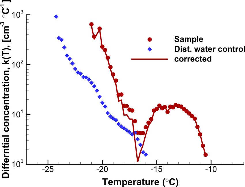
G. Vali: Revisiting the differential freezing nucleus spectra                                                                   1221

                                                                    are good measures of expected ice nucleation in the water
            1       1N       1N                                     samples tested and, for prepared suspensions of known ma-
k(T ) =           ·    ; for        → 0.                     (2)
        X · N (T ) 1T        N (T )                                 terials, k(T ) and K(T ) can readily be used as the basis of
  The cumulative concentration, the integral of k(T ) over          refinements in terms of different models of material proper-
temperature, is given by Eq. (13) in V71 as                         ties and site configurations. The first step in that direction is
                                                                    the active site density description discussed in Sect. 8.
          1
K(T ) =     · [ln No − ln N (T )] ,                          (3)
          X
                                                                    3   Sample data
which can be rewritten in terms of the fraction of drops
frozen f (T ) as                                                    Data from an experiment with a SnomaxTM sample is used
               1                                                    here4 for demonstrating the manner of calculating the dif-
K(T ) = −        · ln[1 − f (T )].                           (4)    ferential concentration. Observed freezing temperatures for
               X
                                                                    507 drops are listed in Table 1. The observations were made
   Because f (T ) is readily obtained in most experiments,          with steady cooling of the drops. Freezing events spread
this direct link to K(T ) is used in a number of publications       over the temperature range from near −4 ◦ C to near −35 ◦ C.
(e.g., DeMott et al., 2017; Hader et al., 2014; Häusler et al.,     Freezing events are most frequent in two temperature re-
2018; Harrison et al., 2018; Kumar et al., 2018; Paramonov          gions, one near −8 ◦ C and the other at the lowest tempera-
et al., 2018; Tarn et al., 2018; Whale et al., 2015) to represent   tures. As can be seen, some temperature values occur more
the results in terms of K(T ).                                      than once due to the finite resolution of the detection and
   A third alternative to obtaining K(T ) is to perform a nu-       recording system used. These characteristics of these data
merical integration of k(T ), remembering that the k(T ) val-       make it useful to demonstrate various points about the cal-
ues here are at discreet T values, not a function:                  culations.
          T
          X
K(T ) =         k(T ) · 1T .                                 (5)
           0                                                        4   Choice of temperature interval
For normalization of k(T ) and K(T ) to unit volume of wa-          The main decision in applying either Eq. (1) or Eq. (2) to
ter, we set X = V , where V is the volume of the drops (as-         experimental results is what numerical values to use for 1T ,
suming drops of uniform sizes). For normalization to unit           taking into account constraints arising from the resolution of
surface area of material dispersed in the drops X = A, with         the temperature measurements and from finite sample sizes.
A denoting the average surface area of particles in each drop.      While all other quantities in Eqs. (1) to (3) are directly mea-
In this case, many authors replace K(T ) with ns (T ), where        sured, 1T is not an empirical value but is one chosen in
ns stands for the site density. See Sect. 8 for further discus-     analysis for desirable representation of the observations. For
sion of the determination of active site density.                   the assumptions involved in the derivation of k(T ), as de-
   Mention has been made already that sample stability is as-       scribed in V71, infinitesimally small intervals δT should be
sumed for valid representations of nucleating activity in any       applied, but this would necessitate infinite, or very large,
quantitative way. Since most INPs are insoluble solid mate-         sample sizes No in order to avoid a large number of intervals
rials, they can be considered stable. Many different potential      without any events. Thus a finite 1T is required. It will be
site configurations, such as crystal steps, dislocations, cracks,   argued that a uniform 1T over the entire temperature range
voids, inclusions, and adsorbed substances, are likely to be        of an experiment is the simplest and most effective choice.
stable. However, since ice nucleation takes place on the sub-       The choice is made, principally, on the basis of sample size
strate surface, stability of the surface is required and that is    (number of drops in the experiment) and not based on instru-
much more difficult to be assured of. The stability require-        mental variables, such as the recording interval of freezing
ment is clearly not fulfilled by samples such as cellulose be-      events.
cause they undergo changes when introduced into water. In              One possible solution for calculating k(T ) with high res-
general, the applicability of active site density may not be        olution would be to use 1N = 1 and with the temperature
known a priori but can be assessed by testing for consistency       intervals between individual freezing events as 1T . This
with different particle loadings, treatments, or other methods.     would yield as many points on the spectrum plot as the num-
   A great advantage of quantifying ice-nucleating ability in       ber of drops. However, this approach would have variable
terms of the spectra defined here is the simplicity of these        1T values, which in turn leads to variations in the calcu-
quantities. No assumptions are needed about intrinsic parti-        lated k(T ) values. The magnitude of each point would de-
cle properties, as for example contact angle, and neither are
the results interpreted in terms of quantities not readily de-         4 These data are from work described in Polen et al. (2018) and
termined independently. While presentation of empirical re-         are used here with kind permission from Ryan Sullivan of Carnegie
sults as counts of INPs may seem overly simple, the spectra         Mellon University.

www.atmos-meas-tech.net/12/1219/2019/                                                 Atmos. Meas. Tech., 12, 1219–1231, 2019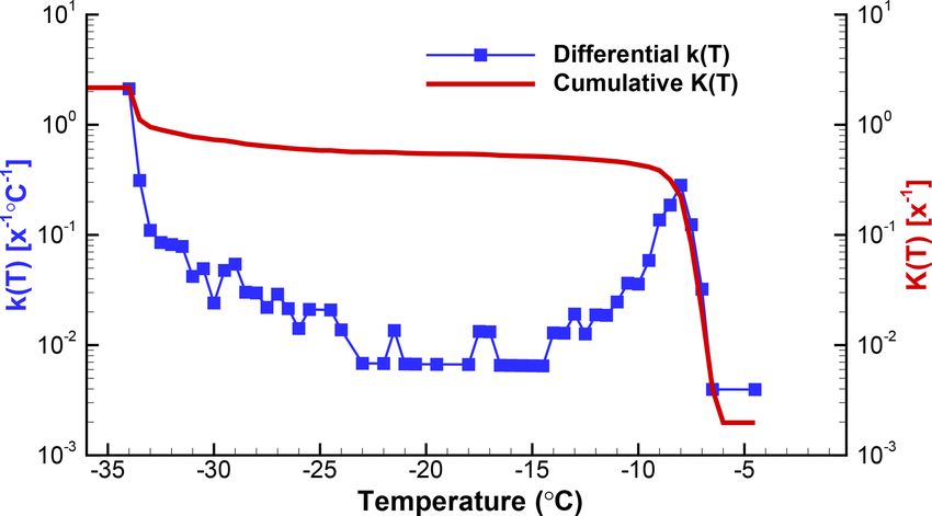
1222                                                                   G. Vali: Revisiting the differential freezing nucleus spectra

Table 1. Observed freezing temperatures for 507 drops of a sample of SnomaxTM dispersed in purified water. Freezing temperatures are
listed in decreasing order. Multiple values are due to time steps of the detection system used. These data are from work described in Polen et
al. (2018).

   −4.42     −6.34      −6.63      −6.71      −6.79      −6.84     −6.84      −6.92      −6.92      −6.92      −7.01     −7.01      −7.01
   −7.01     −7.01      −7.05      −7.14      −7.14      −7.14     −7.14      −7.14      −7.14      −7.14      −7.21     −7.21      −7.21
   −7.21     −7.29      −7.29      −7.29      −7.29      −7.29     −7.34      −7.34      −7.34      −7.43      −7.43     −7.43      −7.43
   −7.50     −7.50      −7.50      −7.50      −7.57      −7.57     −7.57      −7.57      −7.57      −7.57      −7.57     −7.57      −7.57
   −7.57     −7.57      −7.63      −7.63      −7.63      −7.63     −7.63      −7.63      −7.63      −7.63      −7.71     −7.71      −7.71
   −7.71     −7.71      −7.71      −7.71      −7.71      −7.71     −7.71      −7.79      −7.79      −7.79      −7.79     −7.79      −7.79
   −7.79     −7.86      −7.86      −7.86      −7.86      −7.86     −7.86      −7.93      −7.93      −7.93      −7.93     −7.93      −7.93
   −7.93     −7.93      −7.98      −7.98      −7.98      −7.98     −8.05      −8.05      −8.05      −8.05      −8.05     −8.05      −8.05
   −8.05     −8.05      −8.05      −8.11      −8.11      −8.11     −8.21      −8.21      −8.21      −8.21      −8.21     −8.21      −8.21
   −8.27     −8.27      −8.27      −8.27      −8.27      −8.27     −8.27      −8.34      −8.34      −8.40      −8.40     −8.40      −8.40
   −8.40     −8.40      −8.50      −8.50      −8.55      −8.55     −8.55      −8.55      −8.55      −8.55      −8.63     −8.63      −8.70
   −8.70     −8.77      −8.77      −8.77      −8.84      −8.84     −8.84      −8.84      −8.92      −8.99      −8.99     −8.99      −8.99
   −9.06     −9.06      −9.06      −9.06      −9.06      −9.12     −9.21      −9.21      −9.26      −9.35      −9.50     −9.55      −9.55
   −9.71     −9.79      −9.93     −10.00     −10.00     −10.08    −10.13     −10.29     −10.34     −10.57     −10.57    −10.64     −10.71
  −11.29    −11.29     −11.36     −11.94     −11.94     −11.94    −12.02     −12.16     −12.69     −12.69     −12.92    −13.28     −13.48
  −13.56    −13.99     −14.42     −14.94     −15.30     −15.67    −16.03     −16.82     −16.82     −17.19     −17.32    −17.54     −19.30
  −20.40    −20.85     −21.13     −21.13     −21.87     −22.66    −23.73     −23.73     −24.12     −24.17     −24.26    −25.06     −25.34
  −25.42    −25.77     −25.84     −26.07     −26.29     −26.36    −26.51     −26.56     −26.65     −26.93     −27.07    −27.07     −27.30
  −27.65    −27.81     −27.87     −27.94     −28.08     −28.31    −28.36     −28.47     −28.52     −28.60     −28.60    −28.68     −28.80
  −28.89    −28.89     −29.04     −29.16     −29.25     −29.31    −29.46     −29.46     −29.55     −29.69     −29.91    −30.05     −30.05
  −30.21    −30.48     −30.48     −30.48     −30.70     −30.78    −30.78     −30.85     −30.93     −31.00     −31.06    −31.16     −31.16
  −31.32    −31.32     −31.32     −31.32     −31.41     −31.56    −31.63     −31.77     −31.77     −31.83     −31.92    −31.92     −31.92
  −31.97    −32.22     −32.22     −32.28     −32.28     −32.28    −32.33     −32.42     −32.49     −32.49     −32.64    −32.64     −32.70
  −32.78    −32.86     −32.86     −32.86     −32.86     −32.94    −32.94     −32.94     −33.00     −33.00     −33.00    −33.06     −33.06
  −33.14    −33.14     −33.23     −33.23     −33.29     −33.29    −33.29     −33.35     −33.35     −33.35     −33.43    −33.43     −33.43
  −33.43    −33.43     −33.43     −33.49     −33.49     −33.49    −33.49     −33.49     −33.49     −33.59     −33.59    −33.59     −33.59
  −33.59    −33.59     −33.59     −33.59     −33.59     −33.59    −33.65     −33.65     −33.65     −33.65     −33.65    −33.65     −33.65
  −33.65    −33.65     −33.65     −33.71     −33.71     −33.71    −33.71     −33.71     −33.71     −33.71     −33.71    −33.79     −33.79
  −33.79    −33.79     −33.79     −33.79     −33.79     −33.79    −33.79     −33.79     −33.79     −33.79     −33.79    −33.79     −33.79
  −33.79    −33.86     −33.86     −33.86     −33.86     −33.86    −33.86     −33.86     −33.86     −33.86     −33.86    −33.86     −33.86
  −33.86    −33.86     −33.86     −33.86     −33.92     −33.92    −33.92     −33.92     −33.92     −33.92     −33.92    −33.92     −33.92
  −33.92    −33.92     −33.92     −33.92     −33.92     −33.92    −33.92     −33.92     −33.92     −33.92     −33.92    −33.92     −33.92
  −33.92    −33.92     −33.92     −33.92     −33.92     −33.92    −33.92     −34.01     −34.01     −34.01     −34.01    −34.01     −34.01
  −34.01    −34.01     −34.01     −34.01     −34.01     −34.01    −34.01     −34.01     −34.01     −34.01     −34.01    −34.01     −34.01
  −34.01    −34.01     −34.01     −34.07     −34.07     −34.07    −34.07     −34.07     −34.07     −34.07     −34.07    −34.07     −34.07
  −34.07    −34.07     −34.07     −34.07     −34.07     −34.07    −34.07     −34.07     −34.07     −34.07     −34.13    −34.13     −34.13
  −34.13    −34.13     −34.13     −34.13     −34.13     −34.13    −34.13     −34.13     −34.13     −34.13     −34.13    −34.23     −34.23
  −34.23    −34.23     −34.23     −34.23     −34.23     −34.23    −34.23     −34.23     −34.23     −34.23     −34.23    −34.23     −34.23

pend on the temperature interval between successive freez-               recorded. Both the zeros and these minimum nonzero val-
ing events. A given freezing event would correspond to a                 ues are most numerous near −8 ◦ C and near −33 ◦ C where
k(T ) value whose magnitude is changed depending on the                  there are high numbers of freezing occurrences. Larger gaps
previous freezing event in the sample. In effect, the quanti-            become more frequent in the temperature range between the
tive significance of the results would be negated. To see this           two groups due to the sparsity of freezing events. These large
for the SnomaxTM data, the temperature gaps, the differences             and irregular gaps would scramble the k(T ) values.
between the freezing temperatures for successive events, are                Conversely, using a constant value across the range of tem-
shown in Fig. 1. Each point corresponds to one drop and is               peratures covered by the data assures that all points are on the
plotted at the freezing temperature of that drop. The large              same scale. If the observed freezing temperatures are close to
number of points at zero gap size indicates coincidences in              each other, varying the interval width would be compensated
the recorded temperatures for several drops due to the fi-               for by the inclusion of more or fewer events, so the results
nite resolution of the recording system. Another grouping of             would be acceptable, but there is no practical reason for do-
points just below 0.1 is due to the temperature change during            ing that. Thus, it is recommended to select a suitable value
the time intervals with which the number of frozen drops was             for 1T and use it for the whole data set.

Atmos. Meas. Tech., 12, 1219–1231, 2019                                                      www.atmos-meas-tech.net/12/1219/2019/
G. Vali: Revisiting the differential freezing nucleus spectra                                                                       1223

                                                                      Figure 2. Plots of k(T ) for 0.2 and 0.5 ◦ C bin sizes for the data
Figure 1. Temperature gaps between successive freezing events in      from Table 1. The right-hand scale is shifted down slightly to allow
the data given in Table 1. Fewer events in the middle range of tem-   the two plots to be clearly seen. Zero values are indicated for the
peratures produce fewer and larger gaps.                              0.5 ◦ C graph with values below the range covered by the ordinate.
                                                                      The ordinate values are for X = 1 of unspecified dimension, and
                                                                      thus the units are given as [x −1 ◦ C−1 ].

   In the majority of experiments, Ti is irregularly distributed
over the range of all freezing events for a given sample. Thus,       to show these values. For one of the plots in Fig. 2 the zeros
if 1T is chosen too small there will be intervals with zeros          were replaced by a low value well below the range covered
and ones only. That would result in an almost meaningless             by actual data in order to indicate the presence of the zero
representation of the results as k(T ) would also consist of ze-      values. Without this, the presence of zeros, or empty bins,
ros and a uniform small value. The density of points along the        is seen as gaps between points, and as horizontal lines. This
T axis would show some pattern but only in a qualitative way.         matters in judging the significance of the points surrounding
The value chosen for 1T is a compromise between what is               the zeros. Clearly, the dip in k(T ) between −26 and −17 ◦ C
ideal and what is practical. The latter perspective of course         is perceived to be much deeper when the zeros are indicated.
involves judgements over several factors. Most importantly,
these factors are the sample size and associated statistical va-
lidity, the precision with which Ti values are determined, and        5   Calculation of k(T ) and K(T )
the detail in the final spectrum that is believed to hold mean-
ingful information. In view of these conflicting influences,          Once the interval width has been decided, calculation of the
there is no single recipe for setting 1T , but the variations         differential concentration is a straightforward matter, result-
that result in the specific choice do not diminish the objec-         ing in a value of k(T ) for each temperature interval. The cu-
tive value of the derived k(T ) spectrum if normalized to unit        mulative concentration is then also calculated for the same
temperature interval.                                                 temperatures if it is performed by summation of the differ-
   For the sake of simplicity and generality, equal drop vol-         ential values. This is not a requirement; the cumulative spec-
umes are assumed in the calculations here, X is set to unity,         trum can also be calculated without binning of the data and
and the differential concentrations are presented with units          for as many temperatures as wanted.
of ◦ C−1 . Depending on the choice for X, (drop volume,                  Based on the comparison presented in Fig. 2 and on the
particle surface area per drop, mass of particles per drop)           text associated with it, calculations for the SnomaxTM sample
the units of k(T ) will be different, for example ◦ C−1 cm−3 ,        are processed here with 1T = 0.5 ◦ C. The result of that bin-
◦ C−1 µm−2 , or ◦ C−1 g−1 .                                           ning of Ti values is shown in Fig. 3 as a histogram. After bin-
   To illustrate the impacts of the choice of 1T , Fig. 2             ning, values of N (T ) were calculated by stepwise addition
shows the spectra for the SnomaxTM sample with two dif-               of the 1N values from the lowest to the highest temperature,
ferent values. The data shown in Table 1 were binned us-              ending up with No for the first interval with nonzero 1N.
ing 1T = 0.2 ◦ C and 1T = 0.5 ◦ C. For 1T = 0.2 ◦ C there             Performing the accumulation of 1N from lowest to high-
are 51 empty bins (zeros) between −6 and −34 ◦ C. For                 est temperature produces N values at the upper end (warmer
1T = 0.5 ◦ C there are only eight zeros in the same tempera-          temperature) of each interval. The frozen fraction expressed
ture range. Equation (2) was then used to obtain k(T ). Plots         with respect to the lower end (colder temperature) of the in-
of k(T ) shown in Fig. 2 differ, principally, in the degree of        terval is obtained as
noisiness of the data points. Because of the large range of val-                     N (T ) − 1N
ues covered, plots of k(T ) almost always use a logarithmic           f (T ) = 1 −               .                                    (6)
                                                                                          No
ordinate scale. This eliminates the possibility of including
zero values, and special steps need to be taken for the plots

www.atmos-meas-tech.net/12/1219/2019/                                                    Atmos. Meas. Tech., 12, 1219–1231, 2019
1224 G. Vali: Revisiting the differential freezing nucleus spectra Table 2. Differential and cumulative spectra for the SnomaxTM sample with 0.5 ◦ C intervals, as discussed in Sect. 5. Ellipses indicate the range in which not all temperatures are included, for brevity. [1] [2] [3] [4] [5] [6] [7] Temperature Number of events Number unfrozen Number frozen Frozen fraction Differential Cumulative interval center in interval at beginning of interval at end of interval at end of interval per ◦ C at end of interval T 1N N Nf f (T ) k(T ) K(T ) −3.75 0 507 0 0.000 0.000 0.000 −4.25 1 507 1 0.002 0.004 0.002 −4.75 0 506 1 0.002 0.000 0.002 −5.25 0 506 1 0.002 0.000 0.002 −5.75 0 506 1 0.002 0.000 0.002 −6.25 1 506 2 0.004 0.004 0.004 −6.75 8 505 10 0.020 0.032 0.020 −7.25 29 497 39 0.077 0.120 0.080 −7.75 58 468 97 0.191 0.265 0.212 −8.25 35 410 132 0.260 0.178 0.302 −8.75 24 375 156 0.308 0.132 0.368 −9.25 10 351 166 0.327 0.058 0.397 −9.75 6 341 172 0.339 0.036 0.414 −10.25 6 335 178 0.351 0.036 0.432 −10.75 4 329 182 0.359 0.024 0.445 −11.25 3 325 185 0.365 0.019 0.454 −11.75 3 322 188 0.371 0.019 0.463 −12.25 2 319 190 0.375 0.013 0.470 ... ... ... ... ... ... ... ... ... ... ... ... −28.75 7 265 249 0.491 0.054 0.676 −29.25 6 258 255 0.503 0.047 0.699 −29.75 3 252 258 0.509 0.024 0.711 −30.25 6 249 264 0.521 0.049 0.735 −30.75 5 243 269 0.531 0.042 0.756 −31.25 9 238 278 0.548 0.077 0.795 −31.75 9 229 287 0.566 0.080 0.835 −32.25 9 220 296 0.584 0.084 0.877 −32.75 11 211 307 0.606 0.107 0.930 −33.25 27 200 334 0.659 0.290 1.075 −33.75 89 173 423 0.834 1.445 1.798 −34.25 84 84 507 1.000 0.000 1.798 −34.75 0 0 507 1.000 0.000 1.798 −35.25 0 0 507 1.000 0.000 1.798 −35.75 0 0 507 1.000 0.000 1.798 The differential concentration was calculated from Eq. (1) is smaller in magnitude than the differential because the dif- and the cumulative from Eq. (3). Results are given in Table 2. ferential is normalized to degrees Celsius intervals, making The table is given from highest to lowest temperature to make the values, for 1T = 0.5 ◦ C used in this example, double the it match the way the data are obtained in the experiment with value without that normalization. gradual cooling. The temperature in the first column is the Plots of the differential and cumulative spectra are given midpoint of the interval over which the data were evaluated. in Fig. . In this graph, zero values are skipped over to give As indicated in the preceding paragraph, columns [4], [5], the graph a less cluttered appearance. By using the same or- and [7] are shifted by one line with respect to the others in dinate for both plots, the cumulative curve starts lower than order that they refer to the low end of the temperature inter- the differential, as explained above. Normalization to per unit val. These distinctions of interval midpoint and high and low volume of the drops or to site density is a matter of applying ends are somewhat unnecessary considering the magnitude the relevant multiplier to the ordinate values. In this exam- of the interval width but are included here to avoid misin- ple, and in most of this paper, plots of the spectra are shown terpretation of the tabulated data. It is also worth noting that with individual points for each temperature interval. In some at the initial part of the table, the cumulative concentration Atmos. Meas. Tech., 12, 1219–1231, 2019 www.atmos-meas-tech.net/12/1219/2019/
G. Vali: Revisiting the differential freezing nucleus spectra                                                                           1225

Figure 3. Histogram of freezing temperatures and a plot of the frac-   Figure 4. Differential and cumulative spectra for data discussed in
tion of drops frozen for the data from Table 1 (SnomaxTM suspen-       Sect. 5 and displayed in different forms in Figs. 2 and 3. Zeros in the
sion).                                                                 differential spectrum are seen in these plots by larger gaps between
                                                                       adjacent points. The left and right ordinate scales are identical. As
                                                                       mentioned in the text, the cumulative curve starts at a lower value
                                                                       than the differential because the differential is expressed with refer-
cases, it might be desirable to fit algebraic equations to the
                                                                       ence to full degree intervals.
data.
   The effectiveness of transmitting the results of analyses
such as this, as mentioned, depends on the numerous fac-               incorrect only if, for some reason, interactions are expected
tors already discussed. From a purely data-processing per-             among INPs from the different sources. The most relevant
spective, the spectrum with lower resolution is better be-             example of additive behavior, applicable to essentially all ex-
cause it has fewer zero values. No claim is made that the              periments with laboratory preparations, is the addition of the
1T = 0.5 ◦ C choice is optimal. The resulting k(T ) spectrum           background activity to that of the material to be tested. The
still has considerable fluctuations in the middle portion of           water used to prepare suspensions of INPs is never totally
the temperature range. Conversely, the main peak is well re-           free of INPs, and there is potential for further contributions
solved, as is its asymmetric shape. There are many additional          to the “background” by the components of the apparatus used
steps that can be considered for smoothing the data, either at         in the experiment. While extreme care is taken in most cases
the 1N level or in k(T ).                                              to minimize the background, it is always present to greater
   From the point of view of showing what kind of INPs                 or lesser extent. Determination of the background is accom-
were contained in the sample, all the graphs clearly indicate          plished with control experiments.
peaks in activity near −8 ◦ C and near −33 ◦ C. The first peak            The usefulness of a quantitative assessment of the back-
is of greater interest because it is due to the INPs added to          ground activity is demonstrated with the following example5 .
the sample, while the low-temperature activity is due to the           A suspension of soil particles in distilled water, and con-
background related to the supporting surface of the drops and          trol measurements of the distilled water, yielded the frozen
to impurities in the water used to suspend the active INPs.            fraction curves in Fig. 5. From these graphs it would ap-
As a minor detail, it may be noted that the −8 ◦ C peak has            pear that the soil sample data are not reliable much below
a broader tail toward colder temperatures. This feature is             about −18 ◦ C because of the appreciable level of activity in
clearly seen in both of the graphs. Even finer details of the          the control. When the differential spectra are computed and
peak can be seen if the data are processed at higher resolu-           the control is subtracted from the k(T ) values for the sample,
tion, but very little significance can be attached to such de-         the resulting plot shown in Fig. 6 reveals that only in a nar-
tails in light of the sample size, the temperature precision of        row region near −17 ◦ C is the contribution from the distilled
the measurements, and other instrumental factors. Nonethe-             water comparable to the INP activity in the soil. Thus, the
less, it is important to note that the differential spectra can        INP activity in the soil sample below −18 ◦ C can be judged
resolve distinct peaks and thus can provide the type of acute          in a more objective fashion. Just considering this result, it
description of INP activity that is needed in many studies.            would not be baseless to conclude that the soil sample con-
                                                                       tained two types of INPs, those producing the peak centered
                                                                       at −13 ◦ C and those giving rise to high numbers of INPs be-
6   Background correction                                              low −18 ◦ C. In practice, further tests with different amounts
                                                                       of soil in suspension would be useful to judge that conclu-
The differential concentration in a sample with various                sion.
sources of INPs can be assumed to be the sum of the concen-
trations due to each of the sources. This assumption of addi-
tive behavior is likely to hold for many cases and would be               5 This is the same example as was used in Vali (2018).

www.atmos-meas-tech.net/12/1219/2019/                                                      Atmos. Meas. Tech., 12, 1219–1231, 2019
1226 G. Vali: Revisiting the differential freezing nucleus spectra
Figure 5. Observed fractions of droplets frozen for the soil sample
and for the distilled water control, as described in Sect. 6. Data are
Figure 6. Differential spectra for the same data as shown in Fig. 5.
from a single run with 103 drops of 0.01 cm3 volume.
Circle symbols are for the soil sample; diamond symbols are for
the control (blue). The spectrum for the soil sample after correction
for the distilled water background is shown with a line. The magni-
7 Confidence intervals tude of the correction is relatively minor in this case except in the
temperature region between about −14 and −18 ◦ C.
Several sources of error contribute to determining the con-
fidence limits or uncertainty ranges of results derived from
drop-freezing experiments. Temperature accuracy is a minor
contribution in most cases. Acuity of the detection of freez- about those values is the measure sought in the simulation.
ing is a larger concern. These and other error sources need to This can be viewed as if a new set of drops were taken each
be evaluated specifically for each experimental setup. A gen- time from the same bulk sample, or a new set of particles
eral and demanding problem is the evaluation of the statisti- were dispersed into the volume each time, and then a freez-
cal validity of results. That uncertainty, arising from sample ing run performed. Simulation allows as many of these runs
sizes, is of special concern because of the usually large tem- to be carried out as needed to reach a good estimate of the
perature range of the observations and the consequent small variability.
number of freezing events at each temperature. Uncertainty The simulation is relatively simple. The number of events
ranges specific to each temperature can be evaluated using in any given temperature interval can be expected to follow
the k(T ) spectra, as described in the following. a Poisson distribution on repeated testing. This probability
Even with identical drop volumes and with all drops pro- distribution fits the situation because the number of events
duced from the same bulk suspension, considerable spreads per interval is discrete and independent of other intervals,
in freezing temperatures are usually observed. As discussed and the observed numbers can serve as the assumed true val-
earlier, variations in freezing temperatures are associated ues. Hence, taking the observed values of 1N (T ) as the ex-
with specific differences in INPs so that the variations in pectation values λ(T ) and generating a large number, say p,
freezing temperatures indicate a nonrandom distribution of of Poisson-distributed numbers for each temperature interval
the INPs of different activities in the drops. Hence, basic sta- provides independent virtual realizations of the experiment.
tistical methods are not applicable to estimating the confi- The mean value of the 1Ni . . . 1Np numbers in each inter-
dence interval of the k(T ) or K(T ) spectra derived to charac- val will equal λ for that interval, and the standard deviation
terize the INP content. In the absence of many repetitions of will be λ0.5 . However, the Poisson distributions include ze-
the experiments to determine variability, Monte Carlo simu- ros even for mean values greater than zero. The chance of
lations provide a possible solution. In V71, such simulations this reduces as the mean increases; the number of zero val-
were applied to show how the spread in k(T ) spectra is re- ues is e−λ .
duced by increasing sample size. Monte Carlo methods of For a first demonstration of the simulation, a data set with
slightly different configurations were also used in Wright and a modest number of 106 drops is used here. Measured num-
Petters (2013) and in Harrison et al. (2018). bers of freezing events for 1T = 0.5 ◦ C intervals and the cal-
The differential concentration provides a convenient basis culated values of k(T ) are given in Table 3. As can be seen,
for simulations because values of k(T ) for given tempera- the number of events per interval is small and would contain
tures are independent of the values at other temperatures. Use many zeros using a smaller 1T . Values in the second column
of the cumulative concentration derived from the frozen frac- were taken as λ and 100 new sets of 1Ni values generated
tion would be less transparent. The simplest basis for sim- using a Poisson-distributed random number generator in IDL
ulations is the number of freezing events observed in each (Harris Geospatial Solutions, Inc.). From those 100 new sets
temperature interval, 1N (T ). Random variability expected of values, 100 new N (T ) values were derived and k(T ) cal-
Atmos. Meas. Tech., 12, 1219–1231, 2019 www.atmos-meas-tech.net/12/1219/2019/G. Vali: Revisiting the differential freezing nucleus spectra 1227
Table 3. Observed freezing data used as input to the Monte Carlo
simulation described in Sect. 7.
Temperature Number of events k(T )
T 1N = λ per ◦ C
−6.25 3 0.057
−6.75 4 0.079
−7.25 6 0.125
−7.75 5 0.111
−8.25 9 0.216
−8.75 5 0.131
−9.25 4 0.111
−9.75 6 0.179
−10.25 3 0.096 Figure 7. Calculated k(T ) values for 100 iterations of random as-
−10.75 2 0.067 signments of 1N from a Poisson distribution with the λ values
−11.25 2 0.069 shown in Table 3 for each interval. Numbers above the abscissa
−11.75 1 0.035 indicate the number of zero values in the simulation for selected
−12.25 2 0.073 temperatures.
−12.75 6 0.236
−13.25 1 0.042
−13.75 9 0.425
−14.25 12 0.759
−14.75 9 0.850
−15.25 13 2.894
culated using Eq. (1). The simulation results can be used in
many different ways to represent the resulting uncertainties
in the presentations of the empirical results. The scatter in
k(T ) values is an immediate way to show the results. Cu-
mulative spectra K(T ) can also be obtained, as can standard
deviations, or other measures. Figure 8. The 10th to 90th percentile range of k(T ) for the results
Simulated results in terms of k(T ) are shown in Fig. 7. shown in Fig. 7. The green diamonds show the values of k(T ) from
At a few places above the temperature axis, the number of the right-hand column of Table 3 for the observed sequence of freez-
zero values that occurred in the simulation for that inter- ing events. Points just above the abscissa are actually zero values.
val are indicated. In this approach, theP total number No for
any given run is not constrained to λ; the actual number
among the 100 simulated sets varied by 10 %. This variation perature intervals, the confidence limits would have become
alters the simulated k(T ) values at the low end of the tem- narrower at the cost of lower temperature resolution. In the
perature range to some degree but is insignificant at the high case presented here, this would be a reasonable choice even
end. There seems to be little reason to go to that extent or re- though the intuitive approach is to present the data with tem-
finement, but the problem could be eliminated by adjusting λ perature resolution justified by measurement precision. The
for lower temperatures for each choice of 1Ni in successive main limitation is from sample size.
steps. One point of assurance on this score is that the 50th As can be expected, the cumulative spectra are less sensi-
percentile of the simulated k(T ) points is only 3 % off from tive to random variations in the number of freezing events per
those shown in Table 3. temperature interval. To illustrate this point, K(T ) is plotted
The spread of 10 % to 90 % of values at each interval is for the 100 simulations in Fig. 9. Spread here decreases to-
shown in Fig. 8. This example shows roughly a factor of 4 ward lower temperatures and as values for more and more
spread in k(T ) over the whole range of temperatures, worse intervals are summed up. While at −6.25 ◦ C there is a fac-
for those points with low k(T ) and hence also having zero tor of 10 spread in values, near −15 ◦ C the spread is about a
values potentially expected in repetitions. As can be seen for factor of 2. This magnitude of error is for a sample of only
this example, it clearly is not justified to attach too much sig- 103 drops, which is encouraging for experiments in which
nificance to fine details of the spectrum, but there is reason- larger drop numbers are not practical. Larger sample sizes
ably good definition of the broad peak of activity centered can yield lower error ranges, but because the slope of the
on −8 ◦ C and of the rapid rise in numbers below −12 ◦ C. spectrum also has an influence no general statements are pos-
Should the observed data have been binned in larger tem- sible.
www.atmos-meas-tech.net/12/1219/2019/ Atmos. Meas. Tech., 12, 1219–1231, 20191228 G. Vali: Revisiting the differential freezing nucleus spectra
Figure 9. Cumulative spectra for 100 simulations for which differ-
ential spectra are shown in Fig. 7. Figure 10. The 10th to 90th percentile range of k(T ) in 100 simula-
tions for a segment of the spectrum shown in Fig. . Points just above
the abscissa stand for zero values. In contrast with other figures, a
linear ordinate scale is used because of the small range of values
covered. A value of X = 1 is used; actual drop volume of particle
As an illustration of the influence of sample size on the concentration is not accounted for.
confidence intervals for k(T ), the SnomaxTM sample for
which data were presented in Sect. 4 was also used in a
Monte Carlo simulation. The input to the simulation was sample sizes will likely pose the most serious limitation to
extracted from Table 1 for the region near the peak, where reaching statistical significance in such tests.
there are 30–50 events per bin. The simulation results for
100 iterations are shown in Fig. 10 and, as can be seen, the
8 Active site density
range of variation is less than a factor of 2 at the peak. At the
lower k(T ) values, the variability is similar to what is seen in Site density is defined in V15 as “the number of sites causing
Fig. 10. Here too, zero values are plotted along an ordinate nucleation per unit surface area of the INP, or equivalent, as
value of 10−2 . functions of temperature or supersaturation; the quantitative
The examples shown above illustrate one possible way measure of the abundance of sites of different ice nucleating
to assess the confidence limits of k(T ). The simulation ap- effectiveness”. Frequently, for added emphasis, the term is
proach is a realistic and readily envisioned method. Similar given as active site density and denoted as ns . This quantity
results for the confidence ranges could be obtained from ta- has already seen extended use in the literature (e.g., Con-
bles of Poisson distribution using the observed number of nolly et al., 2009; Niedermeier et al., 2015; Beydoun et al.,
events in some experiment as λ for each temperature inter- 2016; Paramonov et al., 2018; Boose et al., 2019). As stated
val. The standard deviation, λ0.5 , is another way to measure in Sect. 2, normalization of the cumulative spectrum by par-
variability. However, it cannot be used in the way it would ticle surface area, using X = A in Eq. (4), leads to ns , most
be for normally distributed values because, for example, the frequently in the inverted form
lower limit of the 95 % range at (λ − 2.14 · λ0.5 ) can be neg-
ative for small λ values and therefore not a physically realis- f (T ) = 1 − exp (−A · ns (T )) . (7)
tic value for expected δN. The main point is that confidence
limits can be delineated and with that the meaning of derived No use has been made in the literature of the concept of dif-
k(T ) spectra quantitatively assessed. The results shown here ferential active site density, although that metric has the same
also demonstrate the need for large sample sizes in order to validity as the cumulative one, and is readily derived from
reduce the variability of the derived spectra. Eq. (2) with the substitution of X = A.
Once sample variability has been estimated, statistical Somewhat unfortunately, the active site density term was
methods are available for comparisons of two samples by introduced in the literature in the cumulative form, i.e., ac-
testing, for example, the equivalence of means (e.g., Chap. 20 tivity summed over all temperatures up to the test value. This
in Blank, 1980). Performing that type of test interval by inter- happened because activity was generally understood to mean
val, as in the previous paragraphs, would test for activity in what is more precisely defined as the cumulative activity.
specific temperature regions. That may indeed be very useful The distinction between cumulative and differential activity
in certain cases but will definitely require large sample sizes. is less widely appreciated. Following the general definitions
More complex methods will need to be considered to make of the differential and cumulative spectra, k(T ) and K(T ),
broader overall comparisons of different samples. Combin- it is useful to define differential and cumulative site density
ing data from larger temperature segments – those of greatest functions ks (T ) and Ks (T ) recognizing that Ks (T ) is exactly
interest – could be helpful, but the strong temperature depen- equivalent to ns (T ). If it were not for the already established
dence of activity may be difficult to weigh adequately. Again, practice one could use the symbols ns (T ) and Ns (T ), but it
Atmos. Meas. Tech., 12, 1219–1231, 2019 www.atmos-meas-tech.net/12/1219/2019/G. Vali: Revisiting the differential freezing nucleus spectra 1229
seems better to avoid the confusion that could result when 9 Summary
comparing results from different publications.
The two expressions for active site density are The differential spectrum, k(T ), is a useful representation of
INP activity in heterogeneous freezing. This article examined
1 1N some of the factors that need to be considered in derivations
ks (T ) = − · ln 1 − , (8)
A · 1T N (T ) of k(T ) for experiments executed with gradual cooling of an
1 array of sample drops taken from the same bulk sample and
Ks (T ) = − · ln[1 − f (T )]. (9) with the freezing of drops at different temperatures recorded.
A
Freezing at a given temperature is taken to indicate the pres-
Use of A as average INP surface area included in each drop ence of INPs active at that temperature. In Sect. 4, the im-
implies some important constraint on when that use is justi- portance of the choice of temperature interval for computing
fied. First of all, it implies that the particles are stable and the spectra was elaborated. Methods of calculation and the
that the determination of A was carried out in the suspen- relation to other derived quantities were presented in Sect. 5.
sion, not in the dry state. The two determinations may differ, Two applications were discussed: Sect. 6 presents a method
for example, if the particles contain some soluble material, or for correcting empirical results for background effects. Cor-
they take up water and change in volume. Examples of aging rection for background is achieved by subtraction of the k(T )
and other effects altering particle effectiveness in water have values. In Sect. 7, a method was described for determination
already been reported (e.g., Emersic et al., 2015). Calcula- of confidence limits for k(T ) using Monte Carlo simulations.
tions of ks or Ks for macromolecule INPs are of questionable Sample size and spectral shape determine the error ranges
value; these materials are best characterized with reference to of k(T ). Lesser uncertainty is associated with the cumulative
the total mass of material or the number of individual macro- spectra. The background correction and the determination of
molecules in suspension, not with reference to surface area. error ranges can significantly augment the value of informa-
As for all of the quantitative characterizations discussed in tion derived from laboratory freezing experiments and can
this paper, temporal stability is assumed, at the minimum on improve model predictions of ice formation in clouds.
the timescale of the experiment.
In addition to the considerations of the previous paragraph,
valid use of an average surface area A also requires that de- Data availability. Raw data of observed freezing temperatures for
viations from the mean value be reasonably small and not be the three samples included in this paper are archived at the Univer-
the dominant source of error in the derived measures of ac- sity of Wyoming under https://doi.org/10.15786/y5xr-pw35 (Sulli-
tivity. Special attention is needed with respect to the larger van and Vali, 2019).
particles in polydisperse samples as these contribute dispro-
portionate fractions of the total surface area. With sufficient
knowledge of the particle size distributions, the error esti-
mated can be derived for deviations from the average. Since
A appears in the pre-factor in the equations for both ks (T )
and Ks (T ), the derived error estimate is valid for all values
of the spectrum.
Dependent on the material constituting the INPs, total sur-
face area may be an inadequate parameter to use in the cal-
culation of the active site density. For example, if only a cer-
tain crystal face contains ice-nucleating sites, the surface area
of that face is the relevant measure to include. Knowledge
of such morphological factors is the goal of many studies;
obtaining ks (T ) or Ks (T ) with variations in experimental
parameters may provide useful insights. Conversely, with-
out sufficient knowledge about particle surface characteris-
tics substantial caveats need to be recognized regarding ac-
tive site density spectra.
www.atmos-meas-tech.net/12/1219/2019/ Atmos. Meas. Tech., 12, 1219–1231, 20191230 G. Vali: Revisiting the differential freezing nucleus spectra
Appendix A: Nomenclature
A Average particle surface area contained in drops; m−2
f (T ) Fraction of sample drops frozen at T
k(T ) Differential nucleus concentration; x −1 ◦ C−1
ks (T ) Differential active site density; m−2 ◦ C−1
K(T ) Cumulative concentration of INPs active at temperatures above T ; x −1
Ks (T ) Cumulative site density on the INPs active at temperatures above T ; m−2
ns (T ) Same as Ks (T )
N (T ) Number of drops not frozen at temperature T
1N Number of freezing events per temperature interval
No Total number of sample drops
T Temperature; ◦ C
Ti Freezing temperature of a drop
X Reference quantity for normalization to unit volume of water, particle surface area, etc., as the case may be.
For generality, corresponding units are indicated in k(T ) and K(T ) as x.
λ Mean value of Poisson distribution, in the current context λ = 1Nobserved
Atmos. Meas. Tech., 12, 1219–1231, 2019 www.atmos-meas-tech.net/12/1219/2019/G. Vali: Revisiting the differential freezing nucleus spectra 1231
Competing interests. The authors declare that they have no conflict sions to detect freezing, Atmos. Meas. Tech., 11, 5629–5641,
of interest. https://doi.org/10.5194/amt-11-5629-2018, 2018.
Häusler, T., Witek, L., Felgitsch, L., Hitzenberger, R., and Grothe,
H.: Freezing on a Chip – A New Approach to Determine Hetero-
Acknowledgements. Ryan Sullivan of Carnegie Mellon University geneous Ice Nucleation of Micrometer-Sized Water Droplets, At-
is thanked for permission to use the data given in Table 1. Thanks mosphere, 9, 140, https://doi.org/10.3390/atmos9040140, 2018.
to the associate editor Wiebke Frey for identifying errors in the Kumar, A., Marcolli, C., Luo, B., and Peter, T.: Ice nucleation
original submission. Hinrich Grothe and the anonymous referee activity of silicates and aluminosilicates in pure water and
made suggestions that were helpful for rounding out some of the aqueous solutions – Part 1: The K-feldspar microcline, At-
arguments. Their questions led to the clarification of some details. mos. Chem. Phys., 18, 7057–7079, https://doi.org/10.5194/acp-
18-7057-2018, 2018.
Edited by: Wiebke Frey Niedermeier, D., Augustin-Bauditz, S., Hartmann, S., Wex, H.,
Reviewed by: Hinrich Grothe and one anonymous referee Ignatius, K., and Stratmann, F.: Can we define an asymp-
totic value for the ice active surface site density for hetero-
geneous ice nucleation?, J. Geophys. Res.-Atmos., 120, 5036–
5046, https://doi.org/10.1002/2014JD022814, 2015.
Paramonov, M., David, R. O., Kretzschmar, R., and Kanji, Z. A.: A
References laboratory investigation of the ice nucleation efficiency of three
types of mineral and soil dust, Atmos. Chem. Phys., 18, 16515–
Beydoun, H., Polen, M., and Sullivan, R. C.: Effect of parti- 16536, https://doi.org/10.5194/acp-18-16515-2018, 2018.
cle surface area on ice active site densities retrieved from Polen, M., Brubaker, T., Somers, J., and Sullivan, R. C.: Clean-
droplet freezing spectra, Atmos. Chem. Phys., 16, 13359–13378, ing up our water: reducing interferences from non-homogeneous
https://doi.org/10.5194/acp-16-13359-2016, 2016. freezing of pure water in droplet freezing assays of ice
Blank, L.: Statistical procedures for engineering, management, and nucleating particles, Atmos. Meas. Tech., 11, 5315–5334,
science, McGraw-Hill Book Company, New York and others, https://doi.org/10.5194/amt-11-5315-2018, 2018.
ISBN 0-07-005851-2, 649 pp., 1980. Sullivan, R. and Vali, G.: Data used in the publication Revisiting the
Boose, Y., Baloh, P., Plötze, M., Ofner, J., Grothe, H., Sierau, differential freezing nucleus spectra derived from drop freezing
B., Lohmann, U., and Kanji, Z. A.: Heterogeneous ice nucle- experiments; methods of calculation, applications and confidence
ation on dust particles sourced from nine deserts worldwide – limits, https://doi.org/10.15786/y5xr-pw35, 2019.
Part 2: Deposition nucleation and condensation freezing, At- Tarn, M. D., Sikora, S. N. F., Porter, G. C. E., O’Sullivan,
mos. Chem. Phys., 19, 1059–1076, https://doi.org/10.5194/acp- D., Adams, M., Whale, T. F., Harrison, A. D., Vergara-
19-1059-2019, 2019. Temprado, J., Wilson, T. W., Shim, J. U., and Murray, B.
Connolly, P. J., Möhler, O., Field, P. R., Saathoff, H., Burgess, J.: The study of atmospheric ice-nucleating particles via mi-
R., Choularton, T., and Gallagher, M.: Studies of heterogeneous crofluidically generated droplets, Microfluid. Nanofluid., 22, 52,
freezing by three different desert dust samples, Atmos. Chem. https://doi.org/10.1007/s10404-018-2069-x, 2018.
Phys., 9, 2805–2824, https://doi.org/10.5194/acp-9-2805-2009, Vali, G.: Quantitative evaluation of experimental results on the het-
2009. erogeneous freezing nucleation of supercooled liquids, J. Atmos.
DeMott, P. J., Hill, T. C. J., Petters, M. D., Bertram, A. K., Tobo, Sci., 28, 402–409, 1971.
Y., Mason, R. H., Suski, K. J., McCluskey, C. S., Levin, E. J. T., Vali, G.: Repeatability and randomness in heterogeneous
Schill, G. P., Boose, Y., Rauker, A. M., Miller, A. J., Zaragoza, J., freezing nucleation, Atmos. Chem. Phys., 8, 5017–5031,
Rocci, K., Rothfuss, N. E., Taylor, H. P., Hader, J. D., Chou, C., https://doi.org/10.5194/acp-8-5017-2008, 2008.
Huffman, J. A., Pöschl, U., Prenni, A. J., and Kreidenweis, S. M.: Vali, G.: Interpretation of freezing nucleation experiments: singu-
Comparative measurements of ambient atmospheric concentra- lar and stochastic; sites and surfaces, Atmos. Chem. Phys., 14,
tions of ice nucleating particles using multiple immersion freez- 5271–5294, https://doi.org/10.5194/acp-14-5271-2014, 2014.
ing methods and a continuous flow diffusion chamber, Atmos. Vali, G., DeMott, P. J., Möhler, O., and Whale, T. F.: Technical
Chem. Phys., 17, 11227–11245, https://doi.org/10.5194/acp-17- Note: A proposal for ice nucleation terminology, Atmos. Chem.
11227-2017, 2017. Phys., 15, 10263–10270, https://doi.org/10.5194/acp-15-10263-
Emersic, C., Connolly, P. J., Boult, S., Campana, M., and Li, 2015, 2015.
Z.: Investigating the discrepancy between wet-suspension- Vali, G.: Comment on the quantitative evaluation of background
and dry-dispersion-derived ice nucleation efficiency of noise in drop freezing experiments, Atmos. Meas. Tech. Dis-
mineral particles, Atmos. Chem. Phys., 15, 11311–11326, cuss., https://doi.org/10.5194/amt-2018-134-SC1, 2018.
https://doi.org/10.5194/acp-15-11311-2015, 2015. Whale, T. F., Murray, B. J., O’Sullivan, D., Wilson, T. W., Umo, N.
Hader, J. D., Wright, T. P., and Petters, M. D.: Contribution S., Baustian, K. J., Atkinson, J. D., Workneh, D. A., and Morris,
of pollen to atmospheric ice nuclei concentrations, Atmos. G. J.: A technique for quantifying heterogeneous ice nucleation
Chem. Phys., 14, 5433–5449, https://doi.org/10.5194/acp-14- in microlitre supercooled water droplets, Atmos. Meas. Tech., 8,
5433-2014, 2014. 2437–2447, https://doi.org/10.5194/amt-8-2437-2015, 2015.
Harrison, A. D., Whale, T. F., Rutledge, R., Lamb, S., Tarn, M. Wright, T. P. and Petters, M. D.: The role of time in heterogeneous
D., Porter, G. C. E., Adams, M. P., McQuaid, J. B., Morris, freezing nucleation, J. Geophys. Res.-Atmos., 118, 3731–3743,
G. J., and Murray, B. J.: An instrument for quantifying hetero- https://doi.org/10.1002/jgrd.50365, 2013.
geneous ice nucleation in multiwell plates using infrared emis-
www.atmos-meas-tech.net/12/1219/2019/ Atmos. Meas. Tech., 12, 1219–1231, 2019You can also read