Magnetic Biomonitoring as a Tool for Assessment of Air Pollution Patterns in a Tropical Valley Using Tillandsia sp.
←
→
Page content transcription
If your browser does not render page correctly, please read the page content below
atmosphere
Article
Magnetic Biomonitoring as a Tool for Assessment of
Air Pollution Patterns in a Tropical Valley Using
Tillandsia sp.
Daniela Mejía-Echeverry 1 , Marcos A. E. Chaparro 2, * ID , José F. Duque-Trujillo 1    ID
                                                                                             ,
Mauro A. E. Chaparro 3 and Ana G. Castañeda Miranda 2
 1   Escuela de Ciencias, Departamento de Ciencias de la Tierra, Universidad EAFIT,
     Carrera 49 7 Sur 50 Av. Las Vegas, 3300 Medellín, Colombia; dmejiae1@gmail.com (D.M.-E.);
     jduquetr@eafit.edu.co or jduquetr@gmail.com (J.F.D.-T.)
 2   Centro de Investigaciones en Física e Ingeniería del Centro de la Provincia de Buenos Aires
     (CIFICEN, CONICET-UNCPBA), Pinto 399, B7000GHG Tandil, Argentina; agmiranda82@gmail.com
 3   Centro Marplatense de Investigaciones Matemáticas (CEMIM-UNMDP), Consejo Nacional de
     Investigaciones Científicas y Técnicas (CONICET), Deán Funes 3350, B7602AYL Mar del Plata, Argentina;
     chaparromauro76@gmail.com
 *   Correspondence: chapator@exa.unicen.edu.ar; Tel.: +54-249-4385661

 Received: 5 May 2018; Accepted: 19 June 2018; Published: 19 July 2018

 Abstract: Recently, air pollution alerts were issued in the Metropolitan Area of Aburrá Valley (AVMA)
 due to the highest recorded levels of particulate matter (PM2.5 and PM10 ) ever measured. We propose
 a novel methodology based on magnetic parameters and an epiphytic biomonitor of air pollution
 in order to improve the air pollution monitoring network at low cost. This methodology relies
 on environmental magnetism along with chemical methods on 185 Tillandsia recurvata specimens
 collected along the valley (290 km2 ). The highest magnetic particle concentrations were found at
 the bottom of the valley, where most human activities are concentrated. Mass-specific magnetic
 susceptibility (χ) reaches mean (and s.d.) values of 93.5 (81.0) and 100.8 (64.9) × 10−8 m3 kg−1
 in areas with high vehicular traffic and industrial activity, while lower χ values of 27.3 (21.0) ×
 10−8 m3 kg−1 were found at residential areas. Most magnetite particles are breathable in size
 (0.2–5 µm), and can host potentially toxic elements. The calculated pollution load index (PLI, based on
 potentially toxic elements) shows significant correlations with the concentration-dependent magnetic
 parameters (R = 0.88–0.93; p < 0.01), allowing us to validate the magnetic biomonitoring methodology
 in high-precipitation tropical cities and identify the most polluted areas in the AVMA.

 Keywords: Aburrá Valley; environmental magnetism; multivariate statistical analysis; magnetite;
 magnetic particulate matter; pollution index PLI

1. Introduction
     Magnetic biomonitoring studies have gained importance in the field of environmental magnetism
in the last two decades, mainly because this technique has been used as a tool to study the changes
in the pollution load in specific environments, such as urban areas, through magnetic measurements
in a wide range of natural materials [1,2]. Concerning atmospheric pollution, some authors have
demonstrated the importance of magnetic biomonitoring for determining particulate matter pollution
levels in several cities in Central and South America [3–5].
     Most of the magnetic minerals in airborne particulate matter (PM) and total suspended particles
(TSP) come from human activities, termed anthropogenic. PM2.5 , PM10 , and TSP can be deposited and
accumulated in biological surfaces such as lichens, mosses, and tree leaves. When magnetic minerals,

Atmosphere 2018, 9, 283; doi:10.3390/atmos9070283                         www.mdpi.com/journal/atmosphere
Atmosphere 2018, 9, 283                                                                               2 of 19

elements, polycyclic aromatic hydrocarbons (PAHs), polychlorinated biphenyls (PCBs), etc. of such
deposited/accumulated particles are quantified; and these organisms present visible morphological
changes, they are called bioaccumulators or biomonitors [6]. The characterization of minerals as
magnetite, hematite, maghemite, products of fuels burning, or products of brake-linings, road surface,
and tire wear, could convey valuable information about air quality in places where biomonitors have
been growing or transplanted [7–10]. Additionally, the implementation of lichens, mosses, and tree
leaves as biomonitors is useful compared with traditional monitoring mechanisms due to the low cost
and quick analysis [5,11–17].
      The use of organisms to assess environmental impact is relatively widespread. Bioindicators and
biomonitors of environmental impact are used for the purpose of observing changes in biological
processes and the state of communities or species. Indeed, bioindication and biomonitoring techniques
are starting to be used in legal action (e.g., in Europe) because their relevance has already been
recognized by international committees (e.g., for lichens, mosses, and tobacco plants). The terms
biomonitoring and bioindication refer to specific uses. Bioindicators assess biotic response to
environmental stress qualitatively. For instance, the presence, reduction, or absence of a species
from the environment may be a bioindicator. Good indicators are common and abundant; their ecology
and physiology are well understood, and they are sensitive to environmental stress. For example,
exposure to pollutants may result in unspecific reactions by a particular species, which may allow us to
recognize a polluted site and an unpolluted site. Passive bioindicators are recognized as biomonitors.
Tillandsia recurvata L. is a good biomonitor because it is widespread and is an effective accumulator
of pollutants.
      T. recurvata L. is an epiphytic plant from the Bromeliaceae family that usually tends to create
a spheroidal shape and has a basic root system. These plants have foliar trichomes that allow the
absorption of water, nutrients, and dust from the air [18]; since they can colonize trees and cables,
they are available and well distributed in the Aburrá Valley (Colombia). Out of all vascular plants,
these species are considered to be the most tolerant to stress. The Tillandsia spp. have a high efficiency
of water economy, well-developed support structures, and the ability to obtain mineral nutrients from
very diluted resources such as rainwater. The absorption of minerals takes place when the buds are
wet immediately after rain. Tillandsia spp. are widely distributed in America and many of the islands
of the West Indies. These characteristics facilitate the study of their capacity as accumulator of different
pollutants, such as toxic elements, particles, and magnetic minerals [3].
      Properties of T. recurvata and T. capillaris as magnetic biomonitors of atmospheric pollution
have been reported by [3] in Querétaro metropolitan area (México) and by [4] in Córdoba province
(Argentina), respectively. Climatic conditions in those areas are different from AMVA, e.g., the average
annual temperature in Querétaro is 18 ◦ C and it has around 60 days a year with rain. The biomonitor’s
qualities for retaining airborne PM from the environment, even in rainy weather conditions, are
prominent. This species is not cleaned by rain; on the contrary, it retains more pollutants when it is
wet. In the Metropolitan Area of Aburrá Valley this epiphyte is abundant all along the valley, except in
locations exceeding 2000 meters above sea level, where it is scarce or absent. Nevertheless, T. usenoides
seems to be present at these locations.
      Schrimpff [19] conducted the first biomonitoring study in the Aburrá Valley in Colombia with
T. recurvata, assessing heavy metals, PAHs, and chlorinated hydrocarbons. This author obtained
concentration maps and discussed the possible sources of these airborne compounds. Recent studies
have used T. usenoides as an active monitor (using transplants) of heavy metals [20], and later studies
have used lichens at some air quality monitoring stations (REDAIRE) with the aim of determining
air quality [21].
      Given the adverse effect of PM2.5 and PM10 on human health, people living in highly contaminated
cities are more prone to developing breathing and cardiovascular diseases, asthma [22,23], and possibly
mental disorders [24]. In this sense, the implementation of additional methodologies to the regular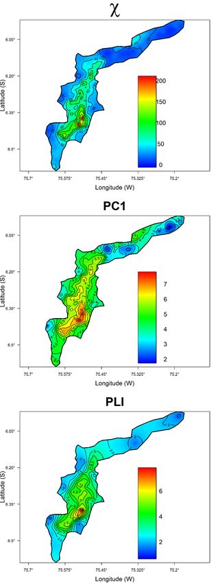
Atmosphere 2018, 9, 283                                                                                      3 of 19

air quality monitoring would be necessary to determine vulnerable places in extensive areas such as
the AVMA.
      The main goal of this study is to assess the airborne PM impact on an extensive and densely
    Atmospherearea
populated      2018,through:
                     9, x FOR PEER
                                (a)REVIEW                                                             3 of 19
                                    the characterization of magnetic particles present in collected samples;
(b) the use of multivariate statistical methods on magnetic and chemical variables in order to identify
    (b) the use of multivariate statistical methods on magnetic and chemical variables in order to
relevant magnetic parameters as potential pollution indicators; and (c) the detection of the most
    identify relevant magnetic parameters as potential pollution indicators; and (c) the detection of the
polluted sites in the AVMA.
    most polluted sites in the AVMA.
2. Experiments
    2. Experiments
2.1. Study Area
    2.1. Study Area
      The Aburrá Valley (a Colombian inter-Andean basin), is a N–S straight valley of 24 km in length
          The Aburrá Valley (a Colombian inter-Andean basin), is a N–S straight valley of 24 km in
and 12 km wide. It is surrounded by mountains that rise up to 1000 m above the bottom of the valley.
    length and 12 km wide. It is surrounded by mountains that rise up to 1000 m above the bottom of
The Aburrá Valley metropolitan area corresponds to a conglomerate of 10 municipalities, whose most
    the valley. The Aburrá Valley metropolitan area corresponds to a conglomerate of 10 municipalities,
populated entity is Medellín (Figure 1). According to [25], AVMA had about 3.8 million inhabitants in
    whose most populated entity is Medellín (Figure 1). According to [25], AVMA had about 3.8 million
2016, concentrated in an 1157 km2 area, reaching222.681 inhabitants per km2 .
    inhabitants in 2016, concentrated in an 1157 km area, reaching 22.681 inhabitants per km2.

      Figure 1. Study area and sampling sites in urban areas of Aburrá Valley (Colombia): Caldas, La Estrella,
         Figure 1. Study area and sampling sites in urban areas of Aburrá Valley (Colombia): Caldas, La
      Sabaneta, Envigado, Itagüí, Medellin, Bello, Copacabana, Girardota and Barbosa.
         Estrella, Sabaneta, Envigado, Itagüí, Medellin, Bello, Copacabana, Girardota and Barbosa.

          Emission inventories from AMVA assign 59% of PM2.5 to vehicle-derived traffic from a fleet of
    1.2 million of vehicles (motorcycles, cars, taxis, buses, and trucks), and an additional 34% of PM2.5 is
    attributed to industrial sources located mostly in the center of the valley [26].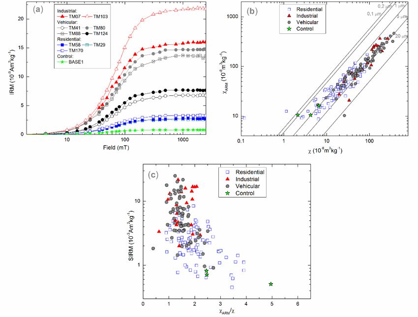
Atmosphere 2018, 9, 283                                                                           4 of 19

      Emission inventories from AMVA assign 59% of PM2.5 to vehicle-derived traffic from a fleet of
1.2 million of vehicles (motorcycles, cars, taxis, buses, and trucks), and an additional 34% of PM2.5 is
attributed to industrial sources located mostly in the center of the valley [26].
      The AVMA has tropical weather, where rainfall is mostly controlled by trade winds, defining two
rainy seasons in the year (April and October). Annual precipitation in the northern part of the valley
is ~1400 mm/year and ~3000 mm/year in the south [27]; such meteorological conditions are ideal
for the accumulation of gases and PM during cloudy periods, occurring mostly between March and
April, when sun radiation cannot reach the valley floor to heat the air, preventing air from rising and
dispersing the air pollutants. The wind regime inside the Aburrá Valley is dominated by pressure
canalization along the valley axis, marked by the Medellín River. During the day, the higher pressure
to the north pushes the wind from north to south (up the valley), coupled with anabatic winds that
push the wind upward from the bottom of the valley. During early night, katabatic winds dominate,
moving the air down the hill and then down the valley (south to north) [28].

2.2. Sampling
      A total of 185 samples of T. recurvata were collected in September 2016 from AVMA urban
areas. The sampling campaign was performed with predominantly sunny weather, and all samples
were collected over a period of four weeks, which minimized the climate variability during sample
collection. Regardless, Tillandsia recurvata has an advantage over tree leaves in that even heavy rains
do not seem to wash away the accumulated particles [3]. A sampling grid was designed in order to
divide the metropolitan area into 50 squares of 6 km2 (Figure 1). Each site was selected according
to epiphyte availability and following the methodology proposed by [3]. Samples were taken in
residential, vehicular, and industrial areas, from trees located along avenues and secondary streets.
Vehicular areas were identified as zones (avenues and freeways) used preferentially by regular traffic
to travel between industrial and residential areas, or between different residential areas. These areas
are affected by traffic, which commonly follows a stop-and-go pattern, resulting in increased brake
and road wear. The size of each specimen of T. recurvata was controlled in order to collect samples with
similar conditions and temporality, choosing individuals of T. recurvata of about 10–15 cm diameter.
A minimum collection height of 1.5 m was used in order to avoid, as much as possible, the influence of
re-suspended soil particles.
      Additionally, in order to obtain a baseline value, three individual control samples were collected
from the city outskirts in a forest area with minimum anthropogenic particle contribution. Samples
were carefully collected using latex gloves and non-magnetic tools to avoid contamination and stored
in paper bags. Samples were then dried in a laboratory furnace at 40 ◦ C in order to avoid mineralogical
transformation. The dried plants were crushed using a hand grinder with a ceramic finish. Grinded
material was packed in plastic containers of 8 cm3 , and firmly pressed to prevent movement during
magnetic measurements.

2.3. Magnetic Measurements
      Magnetic measurements were carried out at the Laboratory of Magnetism and Paleomagnetism
at the CIFICEN-IFAS-UNCPBA (Argentina) and the Environmental Magnetism and Paleomagnetism
Laboratory at EAFIT University (Colombia). Magnetic susceptibility (κ, volume) was measured using
a MS2 susceptibilimeter from Bartington Instruments Ltd. (Witney, England), linked to a MS2B dual
frequency sensor (0.47 and 4.7 kHz). Replicate measurements were done for each sample on the
higher sensitivity range (0.1 × 10⁻⁵ SI); moreover, κ values were corrected for drift through five
measurement cycles (two air readings and three sample readings). The accuracy of the measurement
of κ is 1%. Mass-specific magnetic susceptibility parameter χ was calculated using the κ measurements
and sample weight. Anhysteretic remanent magnetization (ARM) was imparted to all samples
using a device coupled with an alternating field (AF) demagnetizer (Molspin Ltd.), superposing
a DC bias field of 50 and 90 µT to a peak AF of 100 mT and at AF decay rate of 17 µT per cycle.
Atmosphere 2018, 9, 283 5 of 19 The remanent magnetization was measured using a spinner fluxgate magnetometer Minispin (Molspin Ltd., Newcastle upon Tyne, Tyne and Wear, England), which has a noise level
Atmosphere 2018, 9, 283                                                                               6 of 19

2.5. Statistical Analysis
     To analyze the relationship between magnetic parameters and PTE chemistry, a principal
component analysis (PCA) with matrix correlation was analyzed. Before applying this analysis,
a multi-normality analysis was performed. In order to fit it, transformations to multi-normality of [31]
were applied.
     Groups of samples were built based on the principal components coordinates accumulated over
80% of variance, ensuring that the dataset representation is adequate. The fuzzy clustering analysis
(FC) was performed in order to build these groups. The main difference between FC and the classical
clustering method lies in the possibility that a sample belongs to more than one cluster in the FC
method. In the FC method, each sample is assigned a membership value for all clusters as degrees
in the interval (0,1). Furthermore, these membership degrees offer finer detail to the data model [32].
This method is applied in order to determine features along sample transitions between extreme
clusters. The PLI values of the FC were calculated and contrasted with magnetic variables values.
     Based on a previous analysis and looking to show potentially polluted and less polluted sites,
the Ordinary Kriging method (OK) was used to build a prediction map of the most relevant magnetic
parameters and index PLI. The OK is the most popular interpolation spatial method because it considers
knowledge of the spatial variation as represented in the variogram function, and does not require
additional information than the measurement values and their geographic coordinates. The statistical
analyses were performed using the R free software (Vienna, Austria, R version 3.4.0, 2017).

3. Results and Discussion

3.1. Magnetic Properties
      Magnetic parameters and related ratios were determined for all samples. They can be described
as magnetic concentration (χ, ARM and SIRM), magnetic mineralogy (Hcr , S-ratio) and magnetic grain
size (SIRM/χ, χARM /χ and ARM/SIRM) dependent parameters. Such parameters are detailed in the
Supplementary Materials (Table S1).
      According to [33], the magnetic susceptibility parameter roughly approximates the concentration
of magnetic particles in a given sample. Measured χ values varied from 0.1 to 372.9 × 10⁻⁸ m3 kg−1
(Figure 1). The highest concentrations of magnetic particles correspond to sampling sites where land
use was classified as industrial (I) and vehicular (V), with mean values of 100.8 and 93.5 × 10⁻⁸ m3
kg−1 , respectively; while residential (R) areas dominantly show lower mean values of 27.3 × 10⁻⁸ m3
kg−1 (Table 1). ARM and SIRM parameters indicate a wide variation in concentration of ferrimagnetic
minerals that are mainly derived from anthropogenic sources in the AVMA. Minimum and maximum
values vary from 2.9 to 353.0 × 10⁻⁶ A m2 kg−1 for ARM, and from 0.3 to 25.0 × 10⁻³ A m2 kg−1
for SIRM.
      The variability of concentration for the magnetic dependent parameters in relation to different
land uses found in the AVMA is comparable to 38 Indian cities studied by [34], where these authors
reported that the magnetic properties of airborne dust particles collected in artificial containers reported
significant differences between R, V, and I areas. Figure 2a shows different IRM acquisition curves for
samples chosen from R, V, and I areas; the saturation is almost always reached at ~300 mT, showing the
predominance of ferrimagnetic particles [35]. Some samples from industrial areas do not seem to
reach saturation at such fields, indicating the possible contribution of high-coercivity minerals such as
hematite. Despite the acquisition curves not revealing marked mineralogical differences, the SIRM
values for samples V and I are higher with respect to samples R, thus denoting a higher concentration
and accumulation of ferrimagnetic minerals on T. recurvata for these studied sites.
Atmosphere 2018, 9, 283 7 of 19
Table 1. Descriptive statistics of residential, industrial, and vehicular areas. Magnetic concentration- and mineralogy-dependent parameters, elemental concentration,
and pollution index PLI.
ARM SIRM S-ratio SIRM/χ χARM /χ
Samples X (10−8 m3 kg−1 ) Hcr (mT) ARM/SIRM (a.u.)
(10−6 A m2 kg−1 ) (10−3 A m2 kg−1 ) (a.u.) (kA/m) (a.u.)
Residential (n = 91)
min 0.1 2.9 0.3 26.2 0.90 5.5 0.9 0.009
max 88.8 141.8 8.5 40.3 1.00 23.7 10.8 0.023
mean 27.3 38.4 2.5 34.2 10.7 2.1 0.015
s.d. 20.9 24.8 1.6 2.8 3.1 1.2 0.002
Industrial (n = 22)
min 19.7 25.2 2.0 32.5 0.91 6.7 0.6 0.011
max 267.9 282.1 21.7 42.7 1.00 13.5 2.2 0.016
mean 100.8 121.7 9.5 36.4 9.7 1.5 0.013
s.d. 64.9 73.2 5.9 2.4 1.8 0.4 0.001
Vehicular (n = 69)
min 6.2 14.1 0.9 23.8 0.83 5.1 0.4 0.012
max 372.9 353.0 25.0 42.1 1.00 14.7 2.7 0.019
mean 93.5 101.4 7.1 35.6 8.3 1.5 0.015
s.d. 81.0 74.6 5.4 3.8 1.7 0.4 0.001
Control (n = 3)
min 2.1 7.7 0.5 33.6 0.91 12.4 2.5 0.015
max 6.6 13.3 0.8 34.2 0.97 23.8 5.0 0.016
mean 4.3 10.8 0.7 33.8 17.7 3.3 0.016
s.d. 2.2 2.9 0.2 0.3 5.7 1.4 0.001
Ba Co Cr Cu Fe Mo Ni Pb Sb Sn V Zn PLI
Samples
(mg/kg) (mg/kg) (mg/kg) (mg/kg) (mg/kg) (mg/kg) (mg/kg) (mg/kg) (mg/kg) (mg/kg) (mg/kg) (mg/kg) (a.u.)
Residential (n = 19)
min 26.0 0.11 5.3 7.0 8.0 0.2 2.0 2.0 0.9 0.0 1.2 41.0 0.8
max 158.0 8.00 193.0 47.0 183.0 1.2 105.0 38.0 5.6 7.9 19.0 255.0 5.3
mean 80.6 1.24 35.4 19.8 47.1 0.5 15.6 9.7 2.2 1.6 7.8 119.1 2.2
s.d 41.4 1.73 42.0 11.9 37.1 0.3 22.8 8.9 1.2 1.8 4.7 67.1 1.2
Industrial (n = 8)
min 88.0 0.08 20.0 17.0 30.0 0.4 8.0 10.0 2.0 0.9 5.2 86.0 2.0
max 549.0 1.00 122.0 100.0 189.0 2.5 35.0 60.0 9.9 12.0 30.0 577.0 6.9
mean 276.3 0.57 48.1 54.6 85.5 1.6 18.3 27.0 5.9 6.9 15.4 302.4 4.9
s.d 159.9 0.30 33.0 32.6 48.0 0.7 8.5 18.4 2.7 4.1 7.4 166.5 1.8
Vehicular (n = 23)
min 72.0 0.08 9.4 14.0 18.0 0.4 5.0 2.0 0.2 0.7 2.8 71.0 1.8
max 505.0 4.30 174.0 209.0 181.0 6.3 80.0 70.0 20.0 46.0 33.0 333.0 10.7
mean 241.6 0.93 65.6 59.3 87.0 1.6 23.0 24.2 6.4 8.9 13.6 210.5 4.7
s.d 130.3 1.18 39.5 45.9 43.0 1.4 15.9 19.2 4.6 10.9 7.1 77.1 2.1reached at ~300 mT, showing the predominance of ferrimagnetic particles [35]. Some samples from
industrial areas do not seem to reach saturation at such fields, indicating the possible contribution
of high-coercivity minerals such as hematite. Despite the acquisition curves not revealing marked
mineralogical differences, the SIRM values for samples V and I are higher with respect to samples
R, thus denoting
Atmosphere 2018, 9, 283a higher concentration and accumulation of ferrimagnetic minerals on T. recurvata
8 of 19
for these studied sites.
Figure 2. Magnetic
Figure 2. Magnetic parameters
parameters and biplots. (a)
and biplots. (a) Measurements
Measurements of of IRM
IRM (isothermal remanent
(isothermal remanent
magnetization) acquisition for selected samples. (b) King’s Plot (χARM versus χ) for all samples. The
magnetization) acquisition for selected samples. (b) King’s Plot (χARM versus χ) for all samples.
magnetic
The graingrain
magnetic size size
of most of the
of most samples
of the samplesis is
between
between1 1and
and55μm.
µm. (c)
(c) Biplot
Biplot of concentration
of concentration
parameter SIRM
parameter SIRM (IRM
(IRM saturation)
saturation) versus
versus grain
grain size
size dependent
dependent parameter
parameter χχARM/χ /χfor
forall
allsamples.
samples.
ARM
The Hcr values indicate the presence of magnetite-like minerals [35]. According to land use, the
The Hcr values indicate the presence of magnetite-like minerals [35]. According to land use,
mean Hcr (s.d.) values vary in a narrow range, e.g., 34.2 (2.8) mT (R), 35.6 (3.8) mT (V) and 36.4 (2.4)
the mean Hcr (s.d.) values vary in a narrow range, e.g., 34.2 (2.8) mT (R), 35.6 (3.8) mT (V) and
mT (I). Complementary to Hcr, the S ratio is widely used in order to assess the relative contribution
36.4 (2.4) mT (I). Complementary to Hcr , the S ratio is widely used in order to assess the relative
of ferrimagnetic versus antiferromagnetic minerals [36]. Obtained S ratio values evidence the
contribution of ferrimagnetic versus antiferromagnetic minerals [36]. Obtained S ratio values evidence
predominance of low-coercivity phases, with most of values ranging between 0.95 and 1. Although
the predominance of low-coercivity phases, with most of values ranging between 0.95 and 1. Although
magnetic mineralogy in the AVMA is dominated by ferrimagnetic minerals, higher mean values of
magnetic mineralogy in the AVMA is dominated by ferrimagnetic minerals, higher mean values of
Hcr may indicate the presence of high-coercivity minerals [37,38] for different land use areas (Table
Hcr may indicate the presence of high-coercivity minerals [37,38] for different land use areas (Table 1)
1) and such mineral contribution to the IRM is smaller in residential than vehicular and industrial
and such mineral contribution to the IRM is smaller in residential than vehicular and industrial
areas (Figure 2a).
areas (Figure 2a).
The relative magnetic grain-size distribution, inferred from a correlation of χ and χARM
The relative magnetic grain-size distribution, inferred from a correlation of χ and χARM parameters
parameters (King’s Plot) is presented in Figure 2b. Most of the analyzed samples are dominated by
(King’s Plot) is presented in Figure 2b. Most of the analyzed samples are dominated by particles with
magnetic grain-size between 1 and 5 µm, without a strong bias due to land use (Figure 2b). However,
accumulated particles in residential areas and the control site tend to be dominated by finer magnetic
grain sizes (about 1 µm). Moreover, magnetic grains smaller than 1 µm are mostly present in residential
areas located on the AVMA slopes, where usually less vehicular and industrial activity is present. This
behavior is also evidenced by the inter-parametric ratios χARM /χ, SIRM/χ and ARM/SIRM. In these
cases, the mean values of such ratios are higher (indicating finer magnetic grains) for residential and
control areas compared to other land use areas (Table 1). The correlation between a concentration
parameter (SIRM) and a magnetic grain size dependent parameter (χARM /χ), shows that the magnetic
grain size increases in sites with higher SIRM values (SIRM > 9.5 × 10⁻³ A m2 kg−1 ), while lower
SIRM values tend to have smaller magnetic grain size, i.e., higher values of χARM /χ (Figure 2c).ratios χARM/χ, SIRM/χ and ARM/SIRM. In these cases, the mean values of such ratios are higher
(indicating finer magnetic grains) for residential and control areas compared to other land use areas
(Table 1). The correlation between a concentration parameter (SIRM) and a magnetic grain size
dependent parameter (χARM/χ), shows that the magnetic grain size increases in sites with higher
SIRM values
Atmosphere (SIRM
2018, 9, 283 > 9.5 × 10⁻³ A m2 kg−1), while lower SIRM values tend to have smaller magnetic
9 of 19
grain size, i.e., higher values of χARM/χ (Figure 2c).
3.2.
3.2.SEM/EDS
SEM/EDSand
andElemental
ElementalAnalysis
Analysis
In
In order
order to
to characterize
characterize their
their morphology
morphology and and quantify
quantify the
the elemental
elemental composition
composition by by EDS,
EDS,
selected samples, considered representative from the control and three land use areas,
selected samples, considered representative from the control and three land use areas, were were observed
under SEM.
observed under SEM.
Specimens
Specimens of of T.
T. recurvata
recurvata L.
L. collected
collected from
from all
all determined
determined land
land uses
uses (industrial,
(industrial, vehicular,
vehicular,
residential
residential sites and the control areas, Figure 3a–d, respectively) show clear differences in
sites and the control areas, Figure 3a–d, respectively) show clear differences in their
their
leaves
leavesand
andgeneral
generalaspect.
aspect.
Figure 3. SEM observations on T. recurvata samples with different pollution influence from
Figure 3. SEM observations on T. recurvata samples with different pollution influence from industrial
industrial (a), vehicular (b), and residential (c) areas, as well as the control site (d). Composition by
(a), vehicular (b), and residential (c) areas, as well as the control site (d). Composition by EDS of
EDS of Fe-rich particles observed in samples from the industrial area (TM14, e, i), vehicular area
Fe-rich particles observed in samples from the industrial area (TM14, e, i), vehicular area (TM02, f, j),
(TM02, f, j), residential area (TM131, g, k), and control area (BASE 2, h, l) are indicated with particle
residential area (TM131, g, k), and control area (BASE 2, h, l) are indicated with particle metal
metal composition. A morphology and compositional analysis was performed on 49 Fe-rich
composition. A morphology and compositional analysis was performed on 49 Fe-rich particles
particles
on on T.L.
T. recurvata recurvata L.
Iron-rich particles are present at all sites; however, their presence and size increase in the
Iron-rich particles are present at all sites; however, their presence and size increase in the
following order: residential area < vehicular area < industrial area. Forty-nine characteristic
following order: residential area < vehicular area < industrial area. Forty-nine characteristic spherules,
spherules, semi-spherules and irregular Fe-rich particles from 0.3 to 6.6 μm were identified; some of
semi-spherules and irregular Fe-rich particles from 0.3 to 6.6 µm were identified; some of such particles
such particles are shown in Figure 3e–l. Analyzed particles were also revealed to have higher sizes
are shown in Figure 3e–l. Analyzed particles were also revealed to have higher sizes in industrial areas
in industrial areas (mean size = 2.9 μm; n = 20) than in vehicular areas (mean size = 1.2 μm; n = 12)
(mean size = 2.9 µm; n = 20) than in vehicular areas (mean size = 1.2 µm; n = 12) and residential areas
and residential areas (mean size = 1.7 μm; n = 12).
(mean size = 1.7 µm; n = 12).
Iron-oxide-rich spherules are common components of the PM2.5 , PM10 , and TSP emitted from
industrial sites, especially from metallurgical factories, as reported by Chaparro et al. [14]. In the
present study, ~67% of the particles analyzed under SEM were spherules of 0.8–6.4 µm, with a mean
size of ~2.7 µm. Figure 3 gathers some of the most common particle morphology observed in areas
with different land usages: (a) Industrial areas are characterized by perfect iron-oxide spherules with
different sizes (Figure 3e,i; 6.4 µm and, 2.3 µm respectively); (b) Vehicular areas are characterized
by irregular (Figure 3j) and semi-spherical (Figure 3f) particles, where irregular particles range
from 0.3 to 3.1 µm with mean size = 1.2 µm (n = 10); (c) Residential areas are characterized by
semi-spherical and irregular particles ranging from 0.5 to 4.5 µm and mean size of 1.5 µm (n = 9)
(Figure 3g,k); (d) Control sites are characterized by irregular particles ranging from 1 to 2.1 µmAtmosphere 2018, 9, 283 10 of 19
in size (Figure 3h,l). Whole-sample quantitative chemical analysis, using ICP-OES and SEM/EDS
semi-quantitative chemical analysis, were performed on selected samples in order to characterize
both the total elemental contents and the chemical composition of discrete particles in samples from
different land usage sites.
Elemental composition of whole samples from 51 sites was performed by ICP-OES. Results are
listed in the Supplementary Materials (Table S2) and their corresponding descriptive statistics are
shown in Table 1. Most of the elements detected by EDS analysis were then confirmed by ICP-OES
(Table 1, Figure 3). In addition, the ICP-OES data show a significant correlation between the
simultaneous appearance of Fe and V (R = 0.700, p < 0.01), Fe and Cr (R = 0.635, p < 0.01), Fe and
Ni (R = 0.557, p < 0.01), and Fe and Pb (R = 0.546, p < 0.01) (Table 2). Irregular iron-rich particles
coupled with chromium and nickel, as well as metallic iron, were identified along vehicular and
residential areas, showing fine and ultra-fine phase sizes. These are associated with metal structures’
wear and corrosion (due to weather exposure and friction), as well as autoparts’ wear. Iron oxide
particles associated with chromium and zinc were found in vehicular (Figure 3f,j) and residential areas
(Figure 3g,k). In addition, particles composed of iron oxide, chromium, and nickel were found in
samples from residential areas (Figure 3g,k). Spheroidal iron oxide particles are often associated with
casting and welding processes performed in the industry in the study area, e.g., iron oxide spherules
observed in Figure 3e,i correspond to a site (TM14) close to a metallurgical factory.
Control samples also showed the presence of iron-rich particles. Some of these particles are
coarse-sized (5 µm) and have euhedral mineral morphologies. Fine-grained irregular particles
(mean size = 1.2 µm; n = 5) with similar composition were also found in the control site and may be
interpreted as anthropogenic (titano) magnetite or ash derived (Figure 3l).
Elemental contents of Pb, Cr, V, Sn, Sb, Ba, Cu, Zn, and Mo measured on Tillandsias spp. in the
Aburrá Valley (this work) are slightly different from those reported in Medellín city by [19]. New data,
based on 51 selected samples (Table 1 and Supplementary Materials, Table S2), show higher mean
values for Cu and Pb, and lower values for Zn, Ni, and Cr regarding data reported by [19].
Significant correlation was found between simultaneous appearance of Ba and Cu (R = 0.814,
p < 0.01), Ba and Mo (R = 0.808, p < 0.01), Ba and Sb (R = 0.748, p < 0.01), Ba and Fe (R = 0.521, p < 0.01),
Ba and V (R = 0.686, p < 0.01), Ba and Zn (R = 0.686, p < 0.01), and Ba and Pb (R = 0.604, p < 0.01)
(Table 2).
BaSO4 particles of apparent mineral and anthropic type were identified. Because no local
sources of natural barite are known, we assume that all BaSO4 is resulting from pollution. Some of
these particles, found in industrial and vehicular areas, show the cleavage and well-defined angles
characteristic of barite. Barite is mainly used in the glass and pigment industries, as well as for various
processes in the automotive sector. Barite is particularly produced by the wear and tear of braking
systems [39,40]. Spherical particles of BaSO4 (Figure 3i) were also found in industrial areas (Figure 3i).Atmosphere 2018, 9, 283 11 of 19
Table 2. Pearson’s coefficients (R-values) for correlations between magnetic and chemical variables
from T. recurvata samples AMVA (n = 50).
Variable χ ARM SIRM Hcr SIRM/χ χARM /χ ARM/SIRMBa Co Cr
χ 1
ARM 0.955 ** 1
SIRM 0.939 ** 0.991 ** 1
Hcr 0.341 * 1
SIRM/χ −0.474 ** −0.386 ** −0.346 * −0.382 ** 1
χARM /χ −0.460 ** −0.394 ** −0.384 ** −0.300 * 0.844 ** 1
ARM/SIRM −0.370 ** 1
Ba 0.880 ** 0.859 ** 0.846 ** 0.499 ** −0.449 ** −0.423** 1
Co −0.618 ** 1
Cr 0.641 ** 0.698 ** 0.678 ** 0.494 ** 0.576 ** 1
Cu 0.880 ** 0.752 ** 0.725 ** 0.484 ** −0.467 ** −0.438 ** 0.814 ** 0.424 **
Fe 0.785 ** 0.824 ** 0.819 ** −0.295 * −0.354 * −0.318 * 0.521 ** 0.635 **
Mo 0.897 ** 0.780 ** 0.750 ** 0.485 ** −0.434 ** −0.403 ** 0.808 ** 0.432 **
Ni 0.440 ** 0.539 ** 0.526 ** −0.416 ** 0.285 * 0.775 ** 0.930 **
Pb 0.645 ** 0.667 ** 0.666 ** −0.302 * −0.280 * 0.604 ** 0.673 **
Sb 0.828 ** 0.678 ** 0.641 ** 0.506 ** −0.539 ** −0.462 ** 0.748 ** 0.348 *
Sn 0.827 ** 0.668 ** 0.633 ** 0.461 ** −0.401 ** −0.341 * 0.713 ** 0.337 *
V 0.686 ** 0.744 ** 0.752 ** −0.314 * −0.388 ** 0.686 ** 0.630 **
Zn 0.588 ** 0.653 ** 0.658 ** 0.391 ** −0.303 * −0.302 * 0.686 **
PLI 0.933 ** 0.905 ** 0.880 ** 0.323 ** −0.487 ** −0.451 ** −0.192 * 0.891 ** 0.693 **
Variable Cu Fe Mo Ni Pb Sb Sn V Zn PLI
Cu 1
Fe 0.449 ** 1
Mo 0.953 ** 0.479 ** 1
Ni 0.557 ** 1
Pb 0.521 ** 0.546 ** 0.481 ** 0.549 ** 1
Sb 0.895 ** 0.283 * 0.913 ** 0.398 ** 1
Sn 0.938 ** 0.390 ** 0.960 ** 0.393 ** 0.918 ** 1
V 0.541 ** 0.700 ** 0.539 ** 0.498 ** 0.616 ** 0.317 * 0.422 ** 1
Zn 0.515 ** 0.543 ** 0.411 ** 0.514 ** 0.438 ** 0.43 ** 1
PLI 0.868 ** 0.785 ** 0.869 ** 0.510 ** 0.737 ** 0.807 ** 0.778 ** 0.670 ** 0.677 ** 1
significant at the 0.05 level (*) and at the 0.01 level (**).
3.3. Statistical Analysis and Land Use Areas
Descriptive statistics of magnetic variables and PLI relative to I, V, and R land use areas are listed
in Table 1. A multiple pairwise comparison was performed after a Kruskal–Wallis test (Conover Inman
test), in order to analyze the differences between magnetic values on these areas. The results of this
test showed that there are significant differences (p < 0.01) between R and other land usages (I and V)
for all the concentration-dependent magnetic parameters (χ, ARM and SIRM), Hcr (mineralogy) and,
χARM /χ (magnetic size grain). Such significant variation of magnetic parameters for different land use
areas is comparable to the study reported by [34] in R, V, and I areas from India.
Additionally, in this study, the Conover Inman test was performed for PLI; results show that there
are significant differences (p < 0.01) in PTE between R areas and I and V areas; nevertheless, there are
no significant differences between I and V areas.
The PCA with correlation matrix was performed considering all magnetic parameters. Results and
graphical representations are summarized in Table 3 and in the Supplementary Materials (Figure S1).
With the first three principal components it is possible to explain 87% of the observed variance. This
high value of explained variance represents a good reduction of dimension and the high quality of the
dataset representation. The PC1 is mainly defined by the concentration-dependent parameters χ, ARM,
and SIRM, which show high positive correlation. The grain-size-dependent parameters (SIRM/χ andAtmosphere 2018, 9, 283 12 of 19
χARM /χ) contribute both to PC2 and PC1. However, their proportional contribution is higher for PC1
than for PC2.
Table 3. Summary of multivariate analysis of T. recurvata samples. Clusters with similar magnetic
features obtained from fuzzy clustering analysis; and loading values from principal component analysis,
the values in brackets correspond to the correlation with the principal component.
Fuzzy Clustering Analysis Principal Component Analysis
Variable
G1 G2 G3 PC1 PC2 PC3
N I = 0 V = 6 R = 43 I = 6 V = 28 R = 37 I = 16 V = 32 R = 12
χ (10−8 m3 kg−1 ) 11.9 36.3 129.0 23.05 (0.95) 0.69 (0.01) 3.06 (0.03)
ARM (10−6 A m2 kg−1 ) 24.9 50.2 139.4 19.52 (0.81) 4.1 (0.04) 16.26 (0.15)
SIRM (10−3 A m2 kg−1 ) 1.6 3.3 10.2 20.23 (0.84) 7.94 (0.08) 8.44 (0.08)
Hcr (mT) 34.0 34.6 36.4 4.83 (0.2) 17.75 (0.19) 0.49 (0)
SIRM/χ (kA/m) 14.28 9.32 8.18 15.06 (0.62) 23.1 (0.24) 3.24 (0.03)
χARM /χ (a.u.) 2.72 1.73 1.38 14.05 (0.58) 6 (0.06) 25.37 (0.23)
ARM/SIRM (a.u.) 0.016 0.015 0.014 3.27 (0.14) 40.42 (0.43) 43.14 (0.39)
mean PLI (CV%) (a.u.) 1.207 (57.0) 2.386 (78.0) 5.291 (5.2) – – –
PLI min–max (a.u.) 0.820–1.560 1.290–3.620 1.830–10.740 – – –
PC3 is only populated by grain-size-dependent parameter ARM/SIRM. Values of loading and
correlation with PCs are summarized in Table 3. In this way, it is evident that PC1 represents mainly the
concentration of magnetic minerals and grain size and PC2 and PC3 represent the magnetic mineralogy
and grain size of samples.
After executing the PCA, a fuzzy clustering analysis was performed in order to build clusters
of samples based on magnetic parameters only. The clustering was made using three principal
components, based on the accumulated 87% of the dataset variance. The dataset was partitioned
into three clusters, G1 (n = 49) G2 (n = 71), and G3 (n = 60). In this case, the Dunn coefficient was
evaluated and its value was 0.62, indicating that there are some samples sharing characteristics of
different groups. The normalized Dunn coefficient indicates how fuzzy the partition is. A value
of Dunn coefficient close to 0 indicates a very fuzzy clustering, and a value close to 1 indicates a
near-crisp clustering. The cluster G1 shows the lowest values in concentration-dependent magnetic
parameters. This cluster has features related to the softer magnetic minerals and finer magnetic grain
size of the dataset. It is important to note that most of the samples with membership values over 50%
belong to residential areas (i.e., n = 43 out of 46), and G1 lack samples from industrial areas. On the
other hand, cluster G3 presents the opposite features to G1. This group has the highest values in
concentration, coarser grain size, and relatively higher-coercivity mineralogy (the highest value in
the corresponding parameters). This cluster is mostly constituted of samples from industrial areas
(16 out of 22), 32 samples of vehicular areas, and some from residential areas (12 samples). The cluster
G2 is a mix of all areas and values in all magnetic parameters corresponding to intermediate values.
The group is composed by six samples from industrial areas (corresponding to 27% of all samples from
industrial areas), 37 residential samples, and 28 vehicular samples.
The clusters using PLI values were calculated as well; a statistical summary is shown in Table 3.
The G1 has lower concentration, soft mineralogy, and finer magnetic grains; it has the lowest mean
value of PLI of 1.207 (s.d. = 0.680). The G2 has an intermediate value of PLI of 2.386 (s.d. = 1.850).
The cluster G3 has the highest value of concentration, with higher-coercivity mineralogy and coarser
magnetic grains, and has the highest PLI value of 5.291 (s.d. = 0.273).
3.4. Magnetic Biomonitoring
Magnetic properties are well suited as proxies of pollution records [41], with high sensitivity
combined with fast laboratory processing and easy sample preparation. Laboratory instruments are
relatively low cost, and most measurements are non-destructive [42]. An increasing number of studies
use magnetic parameters to assess the air quality in urban areas by means of available biomonitors,Atmosphere 2018, 9, 283 13 of 19
such as lichens [5,14], mosses [12,16,43], and Tillandsia spp. [3,4], among others. In this magnetic
biomonitoring study, in situ growing individuals of T. recurvata, with similar sizes and hence ages,
were collected and used. This allows for assessing the pollution load in an extensive area during
a determined (but not defined) period of accumulation. In such a sense, it is recommended, in the
future, to carry out “active” biomonitoring, i.e., transplanting individuals of T. recurvata from natural
(unpolluted) areas and doing sampling/measurements on determined periods (months, years, etc.) of
interest. Such active biomonitoring not only allows us to define the collection period, but also to assess
changes in time in order to, for example, verify the change in situation after strong anthropic events
taking place in the environment.
Although there are several magnetic parameters, concentration-dependent ones have been used
to evaluate the pollution load in extensive areas, as demonstrated by [44] and others. Such magnetic
parameters can be used as pollution proxies in urban areas if pollution sources (vehicles and industries)
contribute with Fe-rich particles [9,45–47] and if there is a relationship between these particles and PTE.
The present work interprets most of the magnetic particles observed as pollutants coming from
human activities such as industrial processes and vehicular traffic, which are being gathered in different
areas of the AVMA, as observed from parameters χ, ARM, and SIRM (Figure 4). Such preferential
accumulation areas seem to be related to the highly congested roads and industrial infrastructure.
Prediction maps displayed in Figure 4 were built using χ (concentration-dependent magnetic
parameter), PC1 (concentration- and grain-size-dependent magnetic parameters, that is, χ, ARM, SIRM,
SIRM/χ, and χ/χARM ; the first three variables make a higher contribution to the PC according to their
loading values), and pollution index PLI as response variables. The selected variables are based on
statistical results (Table 3) obtained by combining magnetic parameters and chemical determination of
PTE content on each sample.
Constructed variogram functions are of exponential type and their parameters are summarized
in Table 3. Figure 4 shows the distribution of χ, PC1, and PLI obtained for the region. It is necessary
to emphasize that high values of PC1 correspond to areas with a high concentration of magnetic
minerals and high values of PLI to areas with high contents of potentially toxic elements. These areas
are represented by the G3 group from the FC analysis, corresponding to the highest concentration of
magnetic minerals, relatively higher coercivity mineralogy, coarser magnetic grain sizes and higher
pollution index PLI. On the contrary, the lowest values of PC1 correspond to the group G1.
The most polluted sites in the AVMA are located in the south of the valley (Itagüí and
the southern part of downtown Medellin), characterized by increasing concentration-dependent
magnetic parameters: χ (>150.0 × 10⁻⁸ m3 kg−1 ), ARM (>183.8 × 10⁻⁶ A m2 kg−1 ), and SIRM
(>14.0 × 10⁻³ A m2 kg−1 ), as well as pollution index PLI > 6. The emissions of industrial
activities mixed with traffic-derived pollution contribute to higher concentrations of magnetic
particles compared with other areas (Figure 4). The distribution of magnetic particles in the
Aburrá Valley is marked by higher concentrations of magnetic particles in the valley floor
plains, near the Medellin River (mean values of χ, ARM and SIRM are 74.6 × 10⁻⁸ m3 kg−1 ,
85.5 × 10⁻⁶ A m2 kg−1 , and 6.0 × 10⁻³ A m2 kg−1 , respectively), while some residential areas located
at higher elevations present lower concentration related parameters (mean values of χ, ARM and
SIRM are 39.0 × 10⁻⁸ m3 kg−1 , 53.6 × 10⁻⁶ A m2 kg−1 , and 3.7 × 10⁻³ A m2 kg−1 , respectively).
An exception to this result is “El Poblado,” an area located on the southwest flank of the valley.
El Poblado is characterized by a stepped topography, the highest vehicular density per habitant in
the valley, high vehicular flow, and reduced mobility. El Poblado not only has the highest values of
magnetic susceptibility (mean value of χ = 175.0 × 10⁻⁸ m3 kg−1 ), but also has the highest pollution
index (PLI < 10) in the valley.Atmosphere 2018, 9, x FOR PEER REVIEW 15 of 19
transported and biologically accumulated in the human brain, via the olfactory bulb, and associated
Atmosphere 2018, 9, 283 14 of 19
with neurodegenerative diseases such as Alzheimer’s disease [24].
Figure4.4. Prediction
Figure Predictionmap
mapof of
mass-specific magnetic
mass-specific susceptibility
magnetic χ, principal
susceptibility component
χ, principal 1 (PC1: 1χ,
component
ARM, SIRM, SIRM/χ, and χ/χ ARM), and pollution index PLI.
(PC1: χ, ARM, SIRM, SIRM/χ, and χ/χARM ), and pollution index PLI.Atmosphere 2018, 9, 283 15 of 19
In municipalities with small urban centers located in the northern part of the valley (Copacabana,
Girardota, and Barbosa), concentration values (Figure 4) are as low (χ < 30.0 × 10⁻⁸ m3 kg−1 ) as those
found at higher altitudes in Medellín and Envigado. In the southern extreme of the valley (Caldas
and La Estrella), concentration-dependent magnetic parameters increase with respect to the north,
which seems to be related to the high density of textile, chemical, and ceramic industries located in
this area of the valley.
The spatial variation of magnetic grain-size-dependent parameters, such as χARM /χ, SIRM/χ
and ARM/SIRM, shows the dominant presence of finer magnetic particles at higher altitude in
residential or less polluted areas of the valley. Meanwhile, the bottom of the valley is dominated
by a higher concentration of coarser magnetic sized particles. However, most of these particles
are in the breathable size range, between 0.2 and 5 µm (Figure 2b). PM2.5 and PM10 in this range
are harmful for human health because of their ability to be inhaled and reach deep portions of the
respiratory system such as the pulmonary alveoli, making these particles capable of interacting directly
with the bloodstream. Recently, iron-bearing particles have been demonstrated to be transported
and biologically accumulated in the human brain, via the olfactory bulb, and associated with
neurodegenerative diseases such as Alzheimer’s disease [24].
In addition to the potential risk due to the abundance of fine magnetite particles, such minerals can
host PTE such as V, Cr, Ni, Cu, Zn, Mo, Sn, Sb, Ba, and Pb. This is supported by significant correlations
between the magnetic and chemical variables summarized in Table 2. Pearson’s coefficients are
statistically significant at the confidence level 0.01 for concentration-dependent magnetic parameters
and chemical variables, R = 0.60–0.90 p < 0.01. According to the R-values, some PTE have higher
affinity to magnetic particles, in the order Mo > Cu > Ba > Sb > Sn > V > Pb > Cr (Table 2). PLI is
a composite index based on these PTE that correlates significantly with concentration-dependent
magnetic parameters, e.g., R = 0.933, p < 0.01 for χ-PLI (Table 2). In this sense, the spatial variation
of magnetic particles concentration represents, to a greater extent, the air quality with relation to the
particle composition and its dispersion in AVMA (Figure 4).
4. Conclusions
Biomonitoring of air quality in a tropical valley was carried out using Tillandsia recurvata as a
novel bioindicator of air quality. This study provides an overview of air quality from AMVA conditions
using magnetic properties as proxies for potentially toxic element concentration and particle size.
Analysis and interpretation of magnetic properties allow us to reach the following conclusions:
• The χ values vary in the range from 0.1 to 372.9 × 10− 8 m3 kg− 1 , reflecting very low to
very high levels of air pollution in the AMVA. Variation in magnetic particle concentration
estimated from susceptibility is characterized by χ values greater than about 100 × 10−8 m3 kg−1
along the bottom of the valley, while residential areas on the valley slopes have lower values,
of about 30 × 10− 8 m3 kg− 1 . Municipalities located on the northern part of the AVMA, such as
Copacabana, Girardota, and Barbosa, display low magnetic concentration values. Similar values
are only obtained in the residential suburbs of Medellín, located in the highest region of
the hillside.
• Magnetic mineralogy as well as the magnetic susceptibility signal is dominated by ferrimagnetic
phases of low coercivity, i.e., magnetite-like minerals, as indicated by IRM acquisition curves that
reach saturation at fields of about 300 mT, and Hcr mean values of 34.2 mT for (R), 36.4 mT for (I),
and 35.6 mT for (V) areas.
• Average magnetic grain size estimated from magnetic parameters (χARM versus χ,
and anhysteretic ratios) ranges between 0.2 µm and 10 µm, indicating that most of these particles
are 1–5 µm in size. Smaller particles dominate in areas with low pollution loadings. Such results
are in agreement with SEM observations of 49 iron-rich particles that range between 0.3 and 6.6 µm.
Morphologies of Fe-rich particles comprise spherules, semi-spherules, and irregular particles.Atmosphere 2018, 9, 283 16 of 19
Spherules seem to be typical of industrial areas (mean size = 2.7 µm); meanwhile, irregular
particles are common in vehicular (mean size = 1.2 µm) and residential areas (mean size = 1.5 µm).
• The statistical test shows significant differences (p < 0.01) between residential areas and other ones
(I and V) for Hcr and χARM /χ (mineralogy and size-dependent magnetic parameters), as well
as for χ, ARM, and SIRM (magnetic concentration-dependent parameters). Such differences are
a consequence of the topographic effects and anthropogenic activities developed in different
AVMA areas.
• Magnetic proxies of pollution correlate significantly with the concentration of potentially toxic
elements PTE and pollution index PLI (R values up to 0.94, p < 0.01), which indicates, in a broad
sense, that concentration-dependent magnetic parameters reflect air quality in terms of potentially
toxic element particles. Thus, this validates the use of magnetic parameters as pollution proxies
in the AMVA.
• The PCA and fuzzy clustering analysis made between magnetic parameters show clusters
with distinctive magnetic characteristics that represent the pollutant contribution in residential,
vehicular, and industrial areas. Although clusters G1 and G3 are mostly composed of
residential and industrial–vehicular samples, cluster G2 is a mix of samples from all land
use areas and has magnetic parameters corresponding to intermediate values. This fact
indicates the mixed contributions in different land use areas as a consequence of the dispersion
of atmospheric pollutants. The groups of PLI show that the most contaminated sites
(mean PLI = 5.3, Table 3) are those with a high concentration of higher-coercivity magnetic
materials (e.g., χ = 129.0 × 10⁻⁸ m3 kg−1 ) and a relatively coarser grain size. On the other hand,
low pollution impacted sites (mean PLI = 1.2) show the lowest concentration of magnetic particles
(e.g., χ = 11.9 0 × 10−8 m3 kg−1 ), finer magnetic grains, and slightly lower-coercivity.
• T. recurvata has been demonstrated to be a useful biomonitor of air quality in temperate and dry
climates. This study extends it and validates its application in tropical and high precipitation
climates such as the AVMA.
Supplementary Materials: The following are available online at http://www.mdpi.com/2073-4433/9/7/283/
s1. Table S1. Magnetic parameters and elemental determination of Tillandsia recurvata from Aburrá Valley
(Colombia). R: residential; V: vehicular; I: industrial; and Control: BASE. Table S2. Elemental analysis (ICP-OES)
of Tillandsia recurvata from Aburrá Valley. R: residential; V: vehicular; I: industrial; and Control: BASE. Figure S1.
Principal component analysis for AMVA using magnetic variables. PCA biplots show a direct relationship between
χ, ARM and SIRM (right), and a relationship between χARM /χ, SIRM/χ and ARM/SIRM (left).
Author Contributions: D.M.-E. performed the sample collection and magnetic measurements and discussed the
results; M.A.E.C. (Marcos A. E. Chaparro) was primarily responsible for magnetic measurements in the laboratory,
data discussion, and writing the manuscript, J.F.D.-T. led the sampling campaign, refined interpretations,
and contributed to the manuscript preparation; M.A.E.C. (Mauro A. E. Chaparro) contributed to the sampling
design and made the multivariate and geostatistical analysis of data; A.G.C.M. contributed to the sampling
protocol and analyzed the SEM/chemical data.
Funding: This research was funded by the Universidad EAFIT Postgraduate Program, Escuela de Ciencias at
Universidad EAFIT by the internal project #767-000072. This research was partially funded by the Agencia
Nacional de Promoción Científica y Tecnológica ANPCYT grant number PICT-2013-1274.
Acknowledgments: D. Mejía-Echeverry was supported by the Universidad EAFIT Postgraduate Program,
Escuela de Ciencias at Universidad EAFIT. The authors wish to thank Universidad EAFIT, Sistema de Alerta
Temprana (SIATA), Universidad Nacional del Centro de la Provincia de Buenos Aires (UNCPBA), National Council
for Scientific and Technological Research (CONICET), and Centro de Geociencias—Universidad Nacional
Autónoma de México (UNAM) for their financial support. The authors thank both editors and the three
anonymous reviewers whose comments greatly improved the manuscript. They also thank R. Molina-Garza and
J.D. Gargiulo for reviewing the manuscript; Leidy Ortiz, Yenny Valencia; and Daniel Felipe Gómez for sampling
support; and Marina Vega González and CGeo (UNAM) through the Laboratorio de Fluidos Corticales for their
help performing SEM studies.
Conflicts of Interest: The authors declare no conflict of interest.Atmosphere 2018, 9, 283 17 of 19
References
1. Evans, M.; Friedrich, H. Environmental Magnetism: Principles and Applications of Enviromagnetics;
Academic Press: Massachusetts, MA, USA, 2003; p. 299.
2. Chaparro, M.A.E. Estudios de Parámetros Magnéticos de Distintos Ambientes Relativamente Contaminados en
Argentina y Antártida; Geofísica UNAM: Coyoacán, México, 2006; p. 107.
3. Castañeda, M.A.G.; Chaparro, M.A.E.; Chaparro, M.A.E.; Böhnel, H.N. Magnetic properties of Tillandsia
recurvata L. and its use for biomonitoring a Mexican metropolitan area. Ecol. Indic. 2016, 60, 125–136.
[CrossRef]
4. Chaparro, M.A.E.; Castañeda, M.A.G.; Gargiulo, J.D.; Wannaz, E.D.; Böhnel, H.N. Estudios magnéticos en
colectores naturales (Tillandsia capillaris) de contaminantes en Córdoba, Argentina [“Magnetic studies of
pollutants in Tillandsia capillaris from Córdoba, Argentina]. Geos 2014, 34, 70–71.
5. Marié, D.C.; Chaparro, M.A.E.; Irurzun, M.A.; Lavornia, J.M.; Marinelli, C.; Cepeda, R.; Böhnel, H.N.;
Castañeda, M.A.G.; Sinito, A.M. Magnetic mapping of air pollution in Tandil city (Argentina) using the
lichen Parmotrema pilosum as biomonitor. Atmos. Pollut. Res. 2016, 7, 513–520. [CrossRef]
6. Hawksworth, D.L.; Iturriaga, T.; Crespo, A. Líquenes como bioindicadores inmediatos de contaminación y
cambios medio-ambientales en los trópicos. Rev. Iberoam. Micol. 2005, 22, 71–82. [CrossRef]
7. Hunt, C.P.; Moskowitz, B.M.; Banerjee, S.K. Magnetic properties of rocks and minerals. In Rock Physics
& Phase Relations: A Handbook of Physical Constants; Ahrens, T.J., Ed.; American Geophysical Union:
Washington, DC, USA, 1995; Volume 3, pp. 189–204.
8. Maher, B.A.; Thompson, R.; Hounslow, M.W. Introduction. In Quaternary Climates, Environments and
Magnetism; Maher, B.A., Thompson, R., Eds.; Cambridge University Press: Cambridge, UK, 1999; pp. 1–48.
9. Chaparro, M.A.E.; Marié, D.C.; Gogorza, C.S.G.; Navas, A.; Sinito, A.M. Magnetic studies and
scanning electron microscopy X-ray energy dispersive spectroscopy analyses of road sediments, soils,
and vehicle-derived emissions. Stud. Geophys. Geod. 2010, 54, 633–650. [CrossRef]
10. Hofman, J.; Maher, B.A.; Muxworthy, A.R.; Wuyts, K.; Castanheiro, A.; Samson, R. Biomagnetic monitoring
of atmospheric pollution: A review of magnetic signatures from biological sensors. Environ. Sci. Technol.
2017, 51, 6648–6664. [CrossRef] [PubMed]
11. Maher, B.A.; Moore, C.; Matzka, J. Spatial variation in vehicle-derived metal pollution identified by magnetic
and elemental analysis of road side tree leaves. Atmos. Environ. 2008, 42, 364–373. [CrossRef]
12. Fabian, K.; Reimann, C.; McEnroe, S.A.; Willemoes-Wissing, B. Magnetic properties of terrestrial moss
(Hylocomium splendens) along a north-south profile crossing the city of Oslo. Nor. Sci. Total Environ. 2011, 409,
2252–2260. [CrossRef] [PubMed]
13. El-Khatib, A.A.; Abd El-Rahman, A.M.; El-Sheikh, O.M. Biomagnetic monitoring of air pollution using dust
particles of urban tree leaves at Upper Egypt. Assiut Univ. J. Bot. 2012, 41, 111–130.
14. Chaparro, M.A.E.; Lavornia, J.M.; Chaparro, M.A.E.; Sinito, A.M. Biomonitors of urban air pollution:
Magnetic studies and SEM observations corticolous foliose and micro-foliose lichens and their suitability for
magnetic monitoring. Environ. Pollut. 2013, 172, 61–69. [CrossRef] [PubMed]
15. Salo, H.; Mäkinen, J. Magnetic biomonitoring by moss bags for industry-derived air pollution in SW Finland.
Atmos. Environ. 2014, 97, 19–27. [CrossRef]
16. Vukovic, G.; Anici, U.M.; Tomasevic, M.; Samson, R.; Popovic, A. Biomagnetic monitoring of urban air
pollution using moss bags (Sphagnum girgensohnii). Ecol. Indic. 2015, 52, 40–47. [CrossRef]
17. Kodnik, D.; Winkler, A.; Carniel, F.C.; Tretiach, M. Biomagnetic monitoring and element content of lichen
transplants in a mixed land use area of NE Italy. Sci. Total Environ. 2017, 595, 858–867. [CrossRef] [PubMed]
18. Smith, J.A.C. Epiphytic bromeliads. In Vascular Plants as Epiphytes; Springer: Berlin, Germany, 1989;
pp. 109–138.
19. Schrimpff, E. A pollution patterns in two cities of Colombia, South America, according to trace substances
content of an epiphyte (Tillandsia recurvata L.). Water Air Soil Pollut. 1984, 21, 279–315. [CrossRef]
20. Ramírez, M.; Oviedo, J.C.; Salazar, S.; Giraldo, W. Biomonitoreo de metales pesados empleando herramientas
del SIG en el Valle de Aburrá. Rev. Investig. Apl. 2008, 3, 7–14.
21. Jaramillo, M.M.; Botero, L.R. Comunidades liquénicas como bioindicadores de calidad del aire del Valle de
Aburrá. Gest. Ambient. 2010, 13, 97–110.You can also read