Accelerating Deep Learning Inference in Constrained Embedded Devices Using Hardware Loops and a Dot Product Unit
←
→
Page content transcription
If your browser does not render page correctly, please read the page content below
Received August 25, 2020, accepted August 30, 2020, date of publication September 8, 2020, date of current version September 22, 2020.
Digital Object Identifier 10.1109/ACCESS.2020.3022824

Accelerating Deep Learning Inference in
Constrained Embedded Devices Using
Hardware Loops and a Dot Product Unit
JURE VREČA 1 , KARL J. X. STURM 2 , (Student Member, IEEE),
ERNEST GUNGL 1 , (Member, IEEE), FARHAD MERCHANT2 ,
PAOLO BIENTINESI3 , RAINER LEUPERS2 , AND ZMAGO BREZOČNIK                                                        1,   (Member, IEEE)
1 Faculty  of Electrical Engineering and Computer Science, University of Maribor, 2000 Maribor, Slovenia
2 Institute for Communication Technologies and Embedded Systems, RWTH Aachen University, 52056 Aachen, Germany
3 Department of Computing Science, Umeå University, 901 87 Umeå, Sweden

Corresponding author: Jure Vreča (jure.vreca@student.um.si)
This work was supported in part by the Slovenian Research Agency through the Research Program Advanced Methods of Interaction in
Telecommunication under Grant P2-0069.

  ABSTRACT Deep learning algorithms have seen success in a wide variety of applications, such as
  machine translation, image and speech recognition, and self-driving cars. However, these algorithms have
  only recently gained a foothold in the embedded systems domain. Most embedded systems are based
  on cheap microcontrollers with limited memory capacity, and, thus, are typically seen as not capable of
  running deep learning algorithms. Nevertheless, we consider that advancements in compression of neural
  networks and neural network architecture, coupled with an optimized instruction set architecture, could make
  microcontroller-grade processors suitable for specific low-intensity deep learning applications. We propose
  a simple instruction set extension with two main components—hardware loops and dot product instructions.
  To evaluate the effectiveness of the extension, we developed optimized assembly functions for the fully
  connected and convolutional neural network layers. When using the extensions and the optimized assembly
  functions, we achieve an average clock cycle count decrease of 73% for a small scale convolutional neural
  network. On a per layer base, our optimizations decrease the clock cycle count for fully connected layers and
  convolutional layers by 72% and 78%, respectively. The average energy consumption per inference decreases
  by 73%. We have shown that adding just hardware loops and dot product instructions has a significant positive
  effect on processor efficiency in computing neural network functions.

  INDEX TERMS Deep learning, embedded systems, instruction set optimization, RISC-V.

I. INTRODUCTION                                                                                on a microcontroller implanted in the body. The system
Typically, deep learning algorithms are reserved for powerful                                  measures electroencephalography (EEG) data and feeds it to
general-purpose processors, because the convolutional neural                                   the neural network, which determines the seizure activity.
networks routinely have millions of parameters. AlexNet [1],                                   They implemented the neural network on a low power
for example, has around 60 million parameters. Such com-                                       microcontroller from Texas Instruments.
plexity is far too much for memory-constrained microcon-                                          Some embedded system designers work around the
trollers that have memory sizes specified in kilobytes. There                                  dilemma of limited resources by processing neural networks
are, however, many cases where deep learning algorithms                                        in the cloud [4]. However, this solution is limited to areas
could improve the functionality of embedded systems [2].                                       with access to the Internet. Cloud processing also has
For example, in [3], an early seizure detection system is                                      other disadvantages, such as privacy concerns, security, high
proposed, based on a convolutional neural network running                                      latency, communication power consumption, and reliability.
                                                                                               Embedded systems are mostly built around microcontrollers,
    The associate editor coordinating the review of this manuscript and                        because they are inexpensive and easy to use. Recent
approving it for publication was Aysegul Ucar            .                                     advancements in compression of neural networks [5], [6] and

                     This work is licensed under a Creative Commons Attribution 4.0 License. For more information, see https://creativecommons.org/licenses/by/4.0/
VOLUME 8, 2020                                                                                                                                                        165913
J. Vreča et al.: Accelerating Deep Learning Inference in Constrained Embedded Devices
advanced neural network architecture [7], [8] have opened optimize the hardware on which neural networks are running.
new possibilities. We believe that combining these advances As our approach deals mainly with hardware optimization,
with a limited instruction set extension could provide the we will focus on the related approaches for hardware
ability to run low-intensity deep learning applications on optimization, and only discuss briefly the advancements in
low-cost microcontrollers. The extensions must be a good software optimizations.
compromise between performance and the hardware area Because many neural networks, like AlexNet [1],
increase of the microcontroller. VGG-16 [10], and GoogLeNet [11], have millions of
Deep learning algorithms perform massive arithmetic parameters, they are out of the scope of constrained
computations. To speed up these algorithms at a reasonable embedded devices, that have small memories and low clock
price in hardware, we propose an instruction set extension speeds. However, there is much research aimed at developing
comprised of two instruction types—hardware loops and new neural networks or optimizing existing ones, so that they
dot product instructions. Hardware loops, also known as still work with about the same accuracy, but will not take
zero-overhead loops, lower the overhead of branch instruc- up as much memory and require too many clock cycles per
tions in small body loops, and dot product instructions inference. Significant contributions of this research include
accelerate arithmetic computation. the use of pruning [12], quantization [13], and alternative
The main contributions of this article are as follows: number formats such as 8-bit floating-point numbers [14]
• we propose an approach for computing neural network or posit [15], [16]. Pruning of the neural network is based
functions that are optimized for the use of hardware on the fact that many connections in a neural network have
loops and dot product instructions, a very mild impact on the result, meaning that they can
• we evaluate the effectiveness of hardware loops and simply be omitted. On the other hand, the goal of using
dot product instructions for performing deep learning alternative number formats or quantization is to minimize
functions, and the size of each weight. Therefore, if we do not store
• we achieved a reduction in the dynamic instruction weights as 32-bit floating-point values, but instead as 16-
count, an average clock cycle count, and an average bit half-precision floating-point values or in an alternative
energy consumption of 66%, 73%, and 73%, respec- format that uses only 16 or 8 bits (e.g., fixed-point or integer),
tively. we reduce the memory requirements by a factor of 2 or 4. In
order to make deep learning even more resource-efficient,
Deep learning algorithms are used increasingly in we can resort to ternary neural networks (TNNs) with neuron
smart applications. Some of them also run in Internet of weights constrained to {−1, 0, 1} instead of full precision
Things (IoT) devices. IoT Analytics reports that, by 2025, values. Furthermore, it is possible to produce binarized neural
the number of IoT devices will rise to 22 billion [9]. The networks (BNNs) that work with binary values {−1, 1} [17].
motivation for our work stems from the fact that the rise The authors of [18] showed that neural networks using 8-
of the IoT will increase the need for low-cost devices built bit posit numbers have similar accuracy as neural networks
around a single microcontroller capable of supporting deep using 32-bit floating-point numbers. In [5], it is reported
learning algorithms. Accelerating deep learning inference in that, by using pruning, quantization, and Huffman coding,
constrained embedded devices, presented in this article, is our it is possible to reduce the storage requirements of neural
attempt in this direction. networks by a factor of 35 to 49.
The rest of this article is organized as follows. Section II Much research on neural network hardware focuses on a
presents the related work in hardware and software improve- completely new design of instruction set architectures (ISAs)
ments aimed at speeding up neural network computa- built specifically for neural networks. The accelerators
tion. Section III introduces the RI5CY core briefly, and introduced in [19]–[22], and [23] have the potential to offer
discusses hardware loops and the dot product exten- the best performance, as they are wholly specialized. The
sions. Section IV shows our experimental setup. Section V Eyeriss [19] and EIE [20] projects, for example, focus heavily
first presents a simple neural network that we have developed on exploiting the pruning of the neural network, and storing
and ported to our system. It then shows how we have weights in compressed form for minimizing the cost of
optimized our software for the particular neural network memory accesses. The authors of [21] also try to optimize
layers. The empirically obtained results are presented and memory accesses, but use a different strategy. They conclude
discussed in Section VI. Finally, Section VII contains the that new neural networks are too large to be able to hold all the
conclusion and plans for further work. parameters in a single chip; that is why they use a distributed
multi-chip solution, where they try to store the weights as
II. RELATED WORK close to the chip doing the computation as possible, in order
There have been various approaches to speed up deep to minimize the movement of weights. Similarly, in [23], they
learning functions. The approaches can be categorized into developed a completely specialized processor that has custom
two groups. In the first group are approaches which try to hardware units called Layer Processing Units (LPUs). These
optimize the size of the neural networks, or, in other words, LPUs can be thought of as artificial neurons. Before using
optimize the software. Approaches in the second group try to them, their weights and biases must be programmed, and the
165914 VOLUME 8, 2020J. Vreča et al.: Accelerating Deep Learning Inference in Constrained Embedded Devices
activation functions selected. A certain LPU can compute the 32-bit 4-stage in-order RISC-V core, which implements the
output of a particular neuron. This architecture is excellent RV32IMFC instruction set fully. RV32 stands for the 32-bit
for minimizing data movement for weights, but limits the base RISC-V instruction set, I for integer instructions, M for
size of the neural network significantly. The authors of [22] multiplication and division instructions, F for floating-point
realized that many neural network accelerator designs lack instructions, and C for compressed instructions. Addi-
flexibility. It is why they developed an ISA that is flexible tionally, RI5CY supports some custom instructions, like
enough to run any neural network efficiently. The proposed hardware loops. Because we used a floating-point network,
ISA has a total of 43 64-bit instructions, which include we extended the core with our floating-point dot product unit.
instructions for data movement and arithmetic computation We call this core the modified RI5CY core (Fig. 1). It also has
on vectors and matrices. A similar ISA was developed in [24]. an integer dot product unit, but we did not use it. Therefore,
However, because these ISAs are designed specifically for it is not shown for the sake of simplicity. RI5CY is part
neural networks, they are likely unable to be deployed as a of an open-source microcontroller project called PULPino,
single-chip solution (e.g., a microcontroller is needed to drive parts of which we will also use. We call the PULPino
the actuators). To lower the cost of the system and save the microcontroller with the modified RI5CY core the modified
area on the PCB, we sometimes do not want to use a separate PULPino. Both the original and the modified RI5CY core
chip to process the neural network. have 31 general-purpose registers, 32 floating-point registers,
Other works focus on improving the performance of using and a small 128-bit instruction prefetch cache. Fig. 1 details
CPUs to process neural networks. For example, the authors the RI5CY architecture. The non-highlighted boxes show the
of [25] show that adding a mixture of vector arithmetic original RI5CY architecture, while the highlighted fDotp box
instructions and vector data movement instructions to the shows our addition. The two orange-bordered boxes are the
instruction set can decrease the dynamic instruction count general-purpose registers (GPR) and the control-status reg-
by 87.5% on standard deep learning functions. A similar isters (CSR). The violet-bordered boxes represent registers
instruction set extension was developed by ARM—their new between the pipeline stages. The red-bordered boxes show
Armv8.1-M [26] ISA for the Cortex-M based devices is the control logic, including the Hardware-Loop Controller
extended with vector instructions, instructions for low over- ‘‘hwloop control’’, which controls the program counter when-
head loops, and instructions for half-precision floating-point ever a hardware loop is encountered (details are explained
numbers. Unfortunately, as this extension is new, there are in Subsection III-A). The gray-bordered boxes interface
currently no results available on performance improvements. with the outside world. One of them is the load-store-unit
ARM Ltd. published a software library CMSIS-NN [27] (LSU). The boxes bordered with the light blue color are
that is not tied to the new ARMv8.1-M ISA. When running the processing elements. The ALU/DIV unit contains all the
neural networks, CMSIS-NN reduces the cycle count by classic arithmetic-logic functions, including a signed integer
78.3%, and it reduces energy consumption by 79.6%. The division. The MULT/MAC unit allows for signed integer
software library CMSIS-NN achieves these results by using multiplication, as well as multiply-accumulate operations.
an SIMD unit and by quantizing the neural networks. Finally, the fDotp is the unit we added. It is described in
A mixed strategy is proposed in [28]. It presents an Subsection III-B. For more information on the RI5CY core
optimized software library for neural network inference and PULPino, we refer the reader to [29], [30], and [31].
called PULP-NN. This library runs in parallel on ultra-
low-power tightly coupled clusters of RISC-V processors.
PULP-NN uses parallelism, as well as DSP extensions,
to achieve high performance at a minimal power budget.
By using a neural network realized with PULP-NN on
an 8-core cluster, the number of clock cycles is reduced
by 96.6% and 94.9% compared with the current state-of-
the-art ARM CMSIS-NN library, running on STM32L4 and
STM32H7 MCUs, respectively.
Many embedded systems are highly price-sensitive, so the
addition of an extra chip for processing neural networks might
not be affordable. That is why we optimized our software for
a very minimal addition of hardware, which is likely to be
part of many embedded processors. FIGURE 1. The modified RI5CY core. Our extension fDotp is highlighted in
light blue.
III. USED HARDWARE AND INSTRUCTION SET
EXTENSIONS
For studying the benefit of hardware loops, loop unrolling, A. HARDWARE LOOPS
and dot product instructions, we used an open-source RISC-V Hardware loops are powerful instructions that allow execut-
core RI5CY [29], also known as CV32E40P. It is a small ing loops without the overhead of branches. Hardware loops
VOLUME 8, 2020 165915J. Vreča et al.: Accelerating Deep Learning Inference in Constrained Embedded Devices
involve zero stall clock cycles for jumping from the end to the
start of a loop [30], which is why they are more often called
zero-overhead loops. As our application contains many loops,
we use this feature extensively. The core is also capable of
nested hardware loops. However, due to hardware limitation,
the nesting is only permitted up to two levels.
Additionally, the instruction fetch unit of the RI5CY core
is aware of the hardware loops. It makes sure that the
appropriate instructions are stored in the cache. This solution
minimizes unnecessary instruction fetches from the main
memory. FIGURE 2. A schematic representation of the dot product unit.
A hardware loop is defined by a start address, an end
address, and a counter. The latter is decremented with each
iteration of the loop body [30]. Listing 1 shows an assembly IV. EXPERIMENTAL SETUP
code that calculates the factorial of 5 and stores it in the To test the performance of various deep learning algorithms
register x5. Please note that, in RISC-V, x0 is a special register running on the modified RI5CY core, we developed a testing
hardwired to the constant 0. system. We decided to use a Zynq-7000 System-on-a-Chip
(SoC) [32], which combines an ARM Cortex-A9 core and a
field-programmable gate array (FPGA) on the same chip. The
purpose of the ARM Cortex-A9 core is to program, control,
and monitor the modified RI5CY core.
LISTING 1. Assembly code for calculating the factorial of 5 using
hardware loops.
B. DOT PRODUCT UNIT
To speed up dense arithmetic computation, we added an
instruction that calculates a dot product of two vectors with
up to four elements, where each element is a single-precision
FIGURE 3. Block diagram of the system.
floating-point number (32 bits). The output is a scalar
single-precision floating-point number representing the dot
product of the two vectors. The dot product unit is Fig. 3 shows a block diagram of the system. The diagram
shown in Fig. 2. We did not implement any vector load is split into two parts—the processing subsystem (PS) and
instruction; instead, we used the standard load instruction the programmable logic part (PL). On the PL side there
for floating-point numbers. Consequently, this means that is the emulated modified PULPino, and, on the PS side,
we reused the floating-point register file—saving the area the ARM core and the other hard intellectual property
increase of the processor. cores. In between, various interfaces enable data transfer
The ‘×’ and ‘+’ marks in Fig. 2 represent a floating-point between both sides, including a universal asynchronous
multiplier and a floating-point adder, respectively. The unit receiver/transmitter interface (UART), a quad serial periph-
performs two instructions, which we added to the instruction eral interface (QSPI), an advanced extensible interface
set: accelerator coherency port (AXI ACP), and an interrupt line.
• p.fdotp4.s - dot product of two 4-element vectors, Note that all blocks in Fig. 3, except the external DDR
• p.fdotp2.s - dot product of two 2-element vectors. memory, are in the Zynq-7000 SoC chip.
When executing the instruction p.fdotp2.s, the dot product On the PL side (FPGA) of the Zynq-7000 chip, we emu-
unit disconnects the terminals of switch S, automatically, and, lated not only the RI5CY core, but the entire PULPino
similarly, it connects them when executing the instruction microcontroller [33].
p.fdotp4.s. The RI5CY core runs at a relatively low frequency The AXI ACP bus enables high-speed data transfers to the
to reduce energy consumption. Therefore, we can afford that microcontroller. In this configuration, we can get the data
the dot product unit is not pipelined. The result is calculated from the DDR memory, process them, send back the results,
in a single clock cycle. and again get new data from the DDR memory. We use the
165916 VOLUME 8, 2020J. Vreča et al.: Accelerating Deep Learning Inference in Constrained Embedded Devices
QSPI bus to do the initial programming of the PULPino floating-point data type. To compute one pass of the network,
memories and UART for some basic debugging. around 24 thousand multiply-accumulate (MAC) operations
We designed the system in the Verilog hardware descrip- must be performed.
tion language using the Vivado Design Suite 2018.2 inte-
grated development environment provided by Xilinx Inc. A. LOOP UNROLLING
Alongside hardware loops and the dot product unit, we also
V. SOFTWARE tested if loop unrolling could benefit the inference perfor-
To test the efficiency of the designed instruction set mance of our neural network. Loop unrolling is a compiler
optimization, we developed a simple optical character optimization that minimizes the overhead of loops by
recognition (OCR) neural network to recognize handwritten reducing or eliminating instructions that control the loop
decimal digits from the MNIST dataset [34] that contains (e.g., branch instructions). This optimization has the side
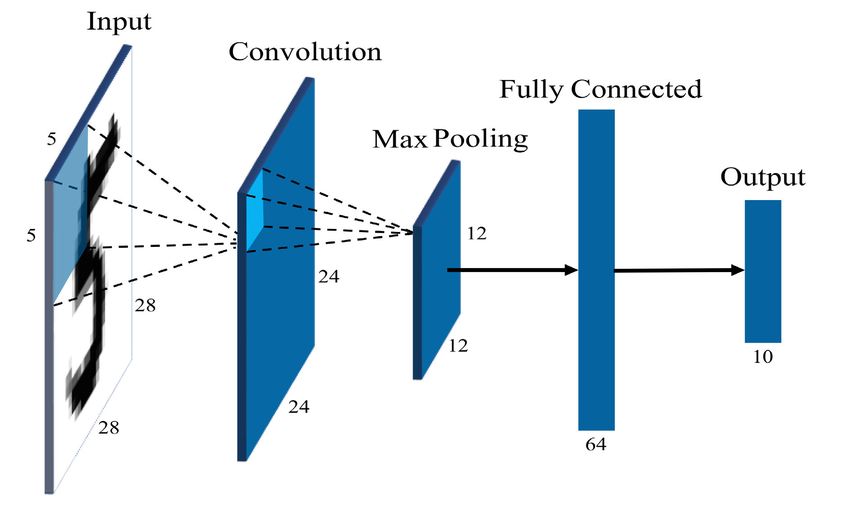
60,000 training data and 10,000 test data. The architecture of effect of increasing code size.
the neural network is given in Table 1 and Fig. 4. The network Algorithm 1 shows a simple for loop that adds up the
was trained in TensorFlow, an open-source software library elements of an array. Algorithm 2 shows the unrolled version
for numerical computations. Using a mini-batch size of 100, of the for loop in Algorithm 1.
the Cross-Entropy loss function, Adam optimization with a
learning rate of 0.01 and 3 epochs of training, recognition
Algorithm 1 A Simple Standard Loop
accuracy 95% was achieved on the test data. For more
information on the neural network, the reader may reference for i = 0; i < n; i = i + 1 do
the supplemental material. State-of-the-art neural networks sum = sum + data[i];
achieve accuracy higher than 99.5% [35]. Compared to end
them, our neural network performs worse, as it has just one
feature map in its only convolutional layer. However, for us,
the accuracy of this neural network is not essential, as we only
need it to test our hardware. Algorithm 2 An Unrolled Loop
for i = 0; i < n; i = i + 4 do
TABLE 1. Architecture of the example neural network. sum = sum + data[i];
sum = sum + data[i + 1];
sum = sum + data[i + 2];
sum = sum + data[i + 3];
end
B. DEEP LEARNING LIBRARY
In order to run our network on the modified RI5CY, we devel-
oped a software library of standard deep learning functions.
We first implemented them by using naive algorithms and
without using the dot product unit. We named this version
of the library the reference version. Following that, we wrote
the optimized assembly code that uses the dot product unit
and hardware loops. We named this version of the library
the optimized assembly version. The naive algorithms were
written in C and could also use hardware loops, as the
compiler is aware of them. Table 2 lists the functions we
implemented in our library. The code can be seen by looking
at the supplemental material.
FIGURE 4. Graphic representation of the example neural network C. FULLY CONNECTED LAYERS
architecture. A fully connected layer of a neural network is computed
as a matrix-vector multiplication, followed by adding a bias
The output of the network is a vector of ten floating-point vector and applying a nonlinearity on each element of the
numbers, which represent the probability that the correspond- resulting vector. In our case, this nonlinearity is the ReLU
ing index of the vector is the digit on the image. In total, function. Equation (1) details the ReLU function for scalar
the network contains 9,956 parameters, which consume input. For a vector input, the function is applied to each
roughly 39 kB of memory space if we use the single-precision element. Equation (2) shows the mathematical operation that
VOLUME 8, 2020 165917J. Vreča et al.: Accelerating Deep Learning Inference in Constrained Embedded Devices
TABLE 2. Functions in our deep learning library.
is being performed to compute one fully connected layer.
f (x) = max(0, x) (1)
E
rE = f (M · Ev + b) (2)
M [m × k] is the matrix of weights of the layer, Ev [k × 1] is
the input vector to the layer, bE [m × 1] is the bias term vector,
f is the nonlinear function, and rE [m × 1] is the output vector,
where m is the number of neurons in the next layer, and k is FIGURE 5. Memory layout for the matrix-vector multiplication algorithm.
the number of neurons in the previous layer or the number of
inputs to the neural network. Fig. 5 shows the placement of the matrix M and vector
In the reference version of the deep learning library, Ev in memory. Each cell in Fig. 5 represents a 32-bit word
we simply used nested for loops to compute the matrix-vector of memory that contains a single-precision floating-point
product, and, following that, we applied the ReLU number. Algorithm 3 shows the pseudocode for executing (3)
nonlinearity. and applying the ReLU nonlinearity. Functions load_vecA()
The optimized assembly version, however, tries to min- and load_vecB() take as input the pointer to the memory
imize the number of memory accesses. Because the dot location from which to load four consecutive scalars.
product unit also operates on vectors, let us first clarify Function load_vecA() is called first—it loads a chunk of the
the terminology. The matrix and vector on which the input vector. Next, the inner for loop traverses through a
matrix-vector multiplication is performed are named the input part of the input matrix. Function load_vecB() loads chunks
matrix M and the input vector Ev, to separate them from the of the input matrix. After loading each chunk, the function
vectors of the dot product unit. Also, the bias vector is denoted dot_prod_vecA_vecB() is called. Algorithm 3 loads data from
by b.E We load in a chunk of the input vector Ev and calculate
memory in the following order. It first loads Ev0 , and then
each product for that chunk. It means that we load the vector vectors m E 0, m E 1, mE 2, m E 3 . Next, it loads Ev1 and vectors m E 4, mE 5,
only once. The size of the chunk is determined by the input E 6, m
m E 7 . The dot products are computed in the following order:
size of the dot product; in our case, it is 4. One problem with E T0 ·Ev0 , m
m E T1 ·Ev0 , m
E T2 ·Ev0 , m
E T3 ·Ev0 , m
E T4 ·Ev1 , m
E T5 ·Ev1 , m
E T6 ·Ev1 , m
E T7 ·Ev1 .
this approach is that the number of matrix columns must be a This way, we only have to load vectors Ev0 and Ev1 once, and,
multiple of four. This problem can be solved by zero-padding at the same time, we have a good spatial locality of memory
the matrix and vector. Equation (3) illustrates this way of accesses.
computing the matrix-vector product for a 4 × 8 input matrix
M , and an 8 × 1 input vector Ev. Subscripted vectors m E Ti , D. CONVOLUTIONAL LAYER
i{0, 1, . . . , 7} and Evj , j{0, 1}, represent the chunks of M and
Both the input to the convolutional layer and its output are
Ev. Each chunk is a vector with four elements. Each chunk of
two-dimensional. To compute a pass of a convolutional layer,
M, m E Ti , is a row vector and the transpose of a column vector
one must compute what is known in signal processing as
E i , because each row of M is composed of two 4-element row
m
a 2D cross-correlation. Following that, a bias is added, and
vectors.
nonlinearity is applied. Equation (4) shows how to compute
T
E 4T
T
E 4T · Ev1 a single element res[x, y] of the two-dimensional output.
E0 m
m mE 0 · Ev0 + m
m E 1T m
E 5T E T · Ev0 + m
· Ev0 = m 1 E 5T · Ev1 out_size
M · Ev = (3) X out_size
E 2T m
E 6T Ev1 E 2T · Ev0 + m
E 6T · Ev1
m m X
res[x, y] = f (b+ fil[i, j] · img[x +i, y+j]) (4)
E 3T m
m E 7T mE 3T · Ev0 + m
E 7T · Ev1 i=1 j=1
165918 VOLUME 8, 2020J. Vreča et al.: Accelerating Deep Learning Inference in Constrained Embedded Devices
Algorithm 3 Computing a Fully Connected Layer With
the ReLU Nonlinearity Applied (dlDensenwReLU)
input : pointer to matrix M of size m × k
input : pointer to vector v of size k
input : pointer to bias b of size m
output: pointer to result vector r of size m
for i = 0 to (k/4) − 1 do
load_vecA(v + i ∗ 4);
for j = 0 to m − 1 do
load_vecB(M + i ∗ m ∗ 4 + j ∗ 4);
r[j] = r[j] + dot_prod_vecA_vecB();
end FIGURE 6. Allocation of the 5 × 5 convolution filter and bias.
end
for i = 0 to m − 1 do Computing the convolutional layer is shown in detail
r[i] = r[i] + b[i]; in Algorithm 4. The functions load_vec_f* load a total
if r[i] < 0 then of 4 consecutive floating-point numbers from the memory
r[i] = 0; location given in the argument to the registers f* to f* + 3.
end The function load_f* loads a single floating-point number to
end register f*. The functions dot_product_f*_f$ compute the dot
product between two chunks in the register file. The first one
starts at f* and ends at f* + 3, and the second one starts at f$
and ends at f$ + 3.
fil is a two-dimensional filter of size fil_size×fil_size, img Fig. 7 shows Algorithm 4 in action at the moment after
is a two-dimensional input array of size img_size × img_size, the first iteration of the inner for loop. The leftmost matrix
b is a scalar bias term, res is the output of size out_size × represents the input image, the middle matrix is the filter, and
out_size, and f is the nonlinear function. Note that more the rightmost matrix is the result matrix. Note that, in Fig. 7,
complicated convolutional neural networks typically have the input image and filter contain only ones and zeros, so that
three-dimensional filters. We show a two-dimensional case anyone can calculate the dot product result quickly (8 in our
for presentation, but to handle three dimensions, we simply case) in the upper-left corner of the result matrix by mental
repeat the procedure for the two-dimensional case. arithmetic. In fact, there are floating-point numbers in each
The reference version of the function dlConv2nwReLU cell.
simply uses nested for loops to compute the convolution in
the spatial domain. It then calls the ReLU function on the
output matrix. Our optimized version tries to optimize the
number of memory accesses. We do that by always keeping
the filter in the register file. We first save the contents of
the register file to the stack. Such an approach enables us
to use the entire register file without breaking the calling
convention used by the compiler. Next, we load the entire 5 ×
5 filter and the bias term into the floating-point register file.
RISC-V has 32 floating-point registers, so we have enough
room in the register file to store the 5 × 5 filter, a chunk FIGURE 7. A visualization of the convolution operation using the dot
of the image, and still have two registers left. Note that product unit.
we again use the word chunk to refer to four floating-point
numbers. Fig. 6(a) and Fig. 6(b) show how we store the 5 VI. RESULTS
× 5 filter and the bias term in memory, and load them into We provide a thorough set of results to give the reader
the floating-point register file. Registers f28-f31 are used to a full picture of the costs and benefits of our proposed
store chunks of the image and registers f9 and f10 to store the instruction set extension. All results of percentage decreases
result. and increases according to the baseline values are rounded to
Having the filter and bias term in the register file, we load whole numbers.
in one chunk of the image at a time and compute the dot
product with the appropriate part of the filter already stored in A. SYNTHESIS RESULTS
the register file. After traversing the entire image, we restore The synthesis was run using the Synopsys Design Compiler
the previously saved register state. We make use of hardware O-2018.06-SP5 and the 90 nm generic core cell library from
loops to implement looping behavior. the United Microelectronics Corporation.
VOLUME 8, 2020 165919J. Vreča et al.: Accelerating Deep Learning Inference in Constrained Embedded Devices
Algorithm 4 Computing the Convolutional Layer With original RI5CY. The area increase is only due to the addition
the ReLU Nonlinearity (dlConv2nwReLU) of the dot product unit, not the hardware loops. The price
input : pointer to image img of size img_size × img_size in the area of adding hardware loops is minor, about
input : pointer to a filter fil of size 5 × 5 3 kGE [29]. Since the RI5CY core already has a floating-point
input : bias b of size 1 unit, we could reduce the area increase by reusing one
input : stride stride floating-point adder and one floating-point multiplier in the
output: result res of size out_size × out_size dot product unit.
Dynamic power consumption was reported by the Design
saveRegisterState(); Compiler using random equal probability inputs, so these
loadFilterAndBiasToRegFile(); results are only approximate. The leakage power con-
out_size = ((img_size − fil_size)/stride) + 1; sumption has more than doubled, but the dynamic power
// x and y get incremented by stride after each consumption has increased only slightly. It is important to
// iteration note that the dynamic power consumption is three orders of
for x = 0 to out_size do magnitude higher, so the total power is still about the same.
for y = 0 to out_size do However, the rise in leakage power might be concerning for
img_slice ← img[x][y]; some low-power embedded systems, that stay most of the
load_vec_f 28_31(img_slice[0][0]); time in standby mode. This concern can be addressed by
res[x][y] = dot_prod_f 0_f 28(); turning off the dot product unit while in standby mode.
load_vec_f 28_31(img_slice[1][0]);
res[x][y] = res[x][y] + dot_prod_f 4_f 28(); B. METHODOLOGY
load_vec_f 28_31(img_slice[2][0]); To gather data about the performance, we used the perfor-
res[x][y] = res[x][y] + dot_prod_f 12_f 28(); mance counters embedded in the RI5CY core. We compared
load_vec_f 28_31(img_slice[3][0]); and analyzed our implementation in the following metrics:
res[x][y] = res[x][y] + dot_prod_f 16_f 28();
• Cycles—number of clock cycles the core was active,
load_vec_f 28_31(img_slice[4][0]);
• Instructions—number of instructions executed,
res[x][y] = res[x][y] + dot_prod_f 20_f 28();
• Loads—number of data memory loads,
load_f 28(img_slice[0][4]);
• Load Stalls—number of load data hazards,
load_f 29(img_slice[1][4]);
• Stores—number of data memory stores,
load_f 30(img_slice[2][4]);
• Jumps—number of unconditional jump instructions
load_f 31(img_slice[3][4]);
executed,
res[x][y] = res[x][y] + dot_prod_f 24_f 28();
• Branch—number of branches (taken and not taken),
load_f 28(img_slice[4][4]);
• Taken—number of taken branches.
res[x][y] = res[x][y] + dot_prod_f 8_f 28();
res[x][y] = res[x][y] + f 11; We compared five different implementations, listed
if res[x][y] < 0 then in Table 4. All of them computed the same result. The
res[x][y] = 0; implementations Fp, FpHw, and FpHwU, use the reference
end library, and implementations FpDotHw and FpDotHwU the
end optimized assembly library. We chose the Fp implementation
end as the baseline. Our goal was to find out how much the
restoreRegisterState(); hardware loops, loop unrolling, and the dot product unit aided
in speeding up the computation. The dot product unit is not
used in all functions of our library, but only in dlDensen,
TABLE 3. Synthesis results. dlDensenwReLU, dlConv2n, and dlConv2nwReLU. How-
ever, these functions represent most of the computing
effort.
For compiling our neural network, we used the modified
GNU toolchain 5.2.0 (riscv32-unknown-elf-). The modified
toolchain (ri5cy_gnu_toolchain) is provided as part of
the PULP platform. It supports custom extensions such
as hardware loops, and applies them automatically when
compiling the neural network with optimizations enabled.
Hardware loops can be disabled explicitly using the compiler
flag -mnohwloop. The neural networks were compiled with
the compiler flags that are listed in Table 4. Even though
Table 3 shows the results of the synthesis. We see that the RI5CY core supports compressed instructions, we did not
the area of the modified RI5CY is 72% larger than the make use of them.
165920 VOLUME 8, 2020J. Vreča et al.: Accelerating Deep Learning Inference in Constrained Embedded Devices
TABLE 4. Different implementations of the program.
C. CODE SIZE COMPARISON In the Fp implementation, where neither hardware loops
We compared the size of the code for the functions listed nor loop unrolling are used, the code size is the smallest.
in Table 2. The results are shown in Table 5. The first three As is predictable, the code with loop unrolling (including our
implementations (Fp, FpHw, and FpHwU) use the reference optimized inline assembly code) is the largest. Nevertheless,
version of the library, while implementations FpDotHw the code size is still quite small, and in the realm of what most
and FpDotHwU use the optimized assembly version of microcontrollers can handle.
the library. The assembly code for a particular (hardware)
implementation is called a function implementation. Note D. FULLY CONNECTED LAYERS
that not all function implementations were written in inline Let us first look at the results for fully connected layers.
assembly, but only the ones whose code sizes are highlighted These layers compute the matrix-vector product, add the bias
blue in Table 5—these function implementations are not and apply the ReLU function. Matrix-vector multiplication
affected by compiler optimizations, and, because of that, takes most of the time. The reader should keep in mind
they are identical at the assembly level. For example, that computing a matrix-vector product is also very memory
the implementations FpDotHw and FpDotHwU use exactly intensive.
the same code for the first four functions. On the other What we are measuring is computing the F3 layer of our
hand, the implementations FpHwU and FpDotHw have the example neural network shown in Table 1. The matrix-vector
same code size for the function dlDensen, but the codes product consists of a matrix with a dimension 64 × 144 and
are not identical. It is just a coincidence. Each of the last a column vector of 144 elements.
three functions (dlMaxPool, dlReLU, and dlSoftmax) has an We ran the same code twenty times with different inputs,
identical function implementation and code size in FpHw and and computed the average of the runs. The averages are
FpDotHw, as well as in FpHwU and FpDotHwU, because displayed in Fig. 8(a) and Fig. 8(b).
the same compiler optimizations apply for implementations Fig. 8(a) compares the number of clock cycles needed to
with or without a dot product unit. Different functions may compute the fully connected layer. Hardware loops alone
be of the same size, as are the sizes of dlConv2n and contribute to a 29% reduction in clock cycles compared to
dlConv2nwReLU for the implementation Fp. Nevertheless, the baseline. A decrease of 72% was achieved with the dot
these function implementations are not identical. The reason product unit included. The result makes sense, since we
for the same size is the fact that the ReLU functionality replaced seven instructions (four multiplications and three
in dlConv2nwReLU is implemented by calling the dlReLU additions) with just one. It would be even better if we could
function, which does not affect the size of the function feed the data to the RI5CY core faster. Let us conclude as
dlConv2nReLU. follows. With our hardware, it takes only one clock cycle to
calculate a single dot product of two vectors of size four, but
TABLE 5. Code size of functions in our deep learning library. All results at least eight clock cycles are needed to fetch the data for
are in bytes. this dot product unit. Because the dot product is calculated
over two vectors of size four and each access takes one clock
cycle, our dot product unit is utilized only 11% of the time.
This result is calculated in (5).
Cycles dot product unit is used 1
= = 11% (5)
Total clock cycles 8+1
The actual utilization is slightly higher, because we reuse
one vector (a chunk) several times, as seen in Algorithm 3.
This fact means that the best possible utilization of our dot
product unit is 1/(4 + 1) = 20%.
VOLUME 8, 2020 165921J. Vreča et al.: Accelerating Deep Learning Inference in Constrained Embedded Devices FIGURE 8. Results for the fully connected layer. The numbers in the columns represent the relative percentages of a given metrics compared to the baseline Fp implementation. Using loop unrolling does not provide any benefit in the branches substantially. Our algorithm, combined with the implementation, neither with nor without the dot product unit. instruction extensions, reduced the number of loads and It slows down FpHwU, and FpDotHwU has about the same stores—as can be seen in Fig. 8(c). The number of loads and amount of clock cycles as FpDotHw. The implementation stores in the FpDotHw implementation was reduced by 36% using hardware loops and loop unrolling (FpHwU) achieved a and 74%, respectively compared to the baseline. 21% reduction in clock cycle count compared to the baseline, but a 29% reduction was achieved using only hardware loops E. CONVOLUTIONAL LAYER (FpHw). The reason is that loop unrolling makes the caching In this Subsection we look at the cost of computing the characteristics of the code much worse (the cache is no longer C1 layer from Table 1. It is a convolution of a 28 × big enough). This effect can be seen by looking at the number 28 input picture with a 5 × 5 filter. We also include of load stalls for the FpHwU implementation in Fig. 8(c). the cost of computing the ReLU function on the resulting The dynamic instruction count comparison can be seen output. We do this because we integrated the ReLU function in Fig. 8(b). Hardware loops contribute a 13% reduction into the convolution algorithm in order to optimize the in dynamic instruction count compared to the baseline. code (dlConv2nwReLU). This layer differs from the fully The optimized inline assembly code for the dot product connected layer, as it is not so constrained by memory unit (FpDotHw) contributed a 63% reduction of the baseline bandwidth. It means that we can use our dot product unit dynamic instruction count. It is a predictable consequence of more effectively. As in the case of the fully connected layer, having one single instruction that calculates a dot product of we were not able to fetch data fast enough to utilize the unit two 4-element vectors instead of seven scalar instructions. entirely. It can be seen in Fig. 9(a) that using our dot product Loop unrolling reduces the dynamic instruction count. unit (FpDotHw) contributed to a 78% reduction of the clock Hardware loops, combined with loop unrolling (FpHwU), cycle count compared to the baseline implementation (Fp). contributed a 22% reduction in the dynamic instruction count Adding just hardware loops to the instruction set (FpHw) compared to the baseline. Unrolling the loop reduces the contributed only a 23% reduction. As in the case of the fully number of loop iterations, but it does not make sense for connected layers, loop unrolling was not effective. hardware loops because there is no overhead. However, not all The dynamic instruction count was again substantially loops can be made into hardware loops due to the limitations lower when using the dot product unit. This fact is a of the RI5CY core. consequence of dot product instruction. By using it, seven The results of auxiliary performance counters are instructions are replaced with only one. In Fig. 9(b) we shown in Fig. 8(c). Our inline assembly code for the see that the dynamic instruction count of the FpDotHw dot product unit (FpDotHw) reduces the number of implementation is reduced by 72% compared to the baseline 165922 VOLUME 8, 2020
J. Vreča et al.: Accelerating Deep Learning Inference in Constrained Embedded Devices

FIGURE 9. Results for the convolutional layer. The numbers in the columns represent the relative percentages of a given metrics compared to the
baseline Fp implementation.

dynamic instruction count. Hardware loops alone (FpHw)                            implementation reduces the clock cycle count by 73%
have a modest impact. They contribute only a 9% reduction                         compared to the baseline. Hardware loops alone (FpHw)
in the dynamic instruction count. Compared to the baseline                        reduce the clock cycle count only by 24%. If we ran our
implementation (Fp), loop unrolling increases the dynamic                         microcontroller at only 10 MHz, we could run a single
instruction count by 7% for computing a convolutional layer                       inference of the neural network in 7.5 ms using the FpDotHw
when not using a dot product unit (FpHwU). The dynamic                            implementation.
instruction count is increased because of the increase in the                        From Fig. 10(b) we can see that the dynamic instruction
number of branches, and it is a consequence of unrolling                          count for the FpDotHw implementation is reduced by 66%
loops with branches inside them (e.g., function dlReLU).                          of the baseline version. The FpHw version also reduces the
   The results of auxiliary performance counters are shown                        dynamic instruction count, but only by 10%.
in Fig. 9(c). The FpDotHw and FpDotHwU implementations                               Fig. 10(c) shows the average results of the auxiliary
reduced the number of loads by 50% compared to the                                performance counters for running a single-pass of the entire
baseline. The number of stores was reduced by 95%.                                neural network. In general, we can say that, by using the
Both results mentioned above are a consequence of our                             dot product unit and the optimized inline assembly code (the
strategy to keep the entire filter and bias term in the                           FpDotHw implementation), we reduced the number of stores
register file. Hardware loops again decreased the number                          by 86%, and the number of loads by 43% compared to the
of branch instructions. The number of branches in the                             baseline (Fp). Since neural networks are very data-intensive,
FpHw implementation was reduced by 91% compared to                                this result is auspicious.
the baseline. Since we used many small loops, hardware
loops are a good idea. The FpDotHw implementation reduced                         G. ENERGY CONSUMPTION
the number of branches even further—by 97% compared to                            We derived the energy consumption results from the ASIC
the baseline. Namely, the only branches in the FpDotHw                            synthesis power results and the number of the executed
implementation come from the ReLU function, while the                             clock cycles for the various implementations. Fig. 11 shows
FpHw function has additional branches for non-hardware                            the energy results of running our entire neural network.
loops. As is the case of fully connected layers, the number                       The results are calculated by multiplying the sum of
of branches increases significantly if loop unrolling is used.                    leakage and dynamic power consumption of the particular
                                                                                  implementation and the time of computing one inference of
F. ENTIRE NEURAL NETWORK                                                          the entire neural network with our microcontroller running
Finally, let us look at the results of running the entire                         at a 10 MHz clock frequency. Energy consumptions for the
example neural network. Fig. 10(a) shows that the FpDotHw                         implementations Fp, FpHw, and FpHwU were calculated

VOLUME 8, 2020                                                                                                                                    165923
J. Vreča et al.: Accelerating Deep Learning Inference in Constrained Embedded Devices
FIGURE 10. Results for the entire neural network. The numbers in the columns represent the relative percentages of a given metrics compared to the
baseline Fp implementation.
by using the power consumption results of the original Our reduction in cycle count is comparable with the 78.3%
RI5CY (see Table 3). For the implementations FpDotHw and reduction achieved by CMSIS-NN [27]. Similarly, the com-
FpDotHwU, energy consumptions were calculated by using bination of hardware loops and dot product instructions
the power consumption results of the modified RI5CY. Note reduced the dynamic instruction count by 66%. Although our
that the results do not include the energy consumption of data reduction in dynamic instruction count is less than the 87.5%
transactions to and from the main memory. reduction gained in [25], we achieved this reduction with a
considerably smaller ISA extension. As embedded systems
are highly price-sensitive, this is an important consideration.
Unfortunately, in [25], the ISA extension hardware cost is not
discussed. A point to emphasize is that our ISA improvements
for embedded systems should be considered together with
other research on compressing neural networks. Getting
the sizes of neural networks down is an essential step in
expanding the possibilities for neural networks in embedded
systems. For example, in [5], it is shown that it is possible to
quantize neural networks to achieve a size reduction of more
FIGURE 11. Energy consumption for one inference of our example neural
than 90%. Another interesting topic for further research is
network. Posit—an alternative floating-point number format, that may
offer additional advantages, as it has an increased dynamic
Adding the dot product unit (FpDotHw) reduced energy
range at the same word size [15], [36]. Because of the
consumption by 73% compared to the baseline. Hardware
improved dynamic range, weights could be stored in lower
loops alone reduced it by 24%, but if loop unrolling was
precision, thus, again, decreasing the memory requirements.
included, the energy consumption dropped by only 10%
Combining the reduced size requirements with low-cost ISA
compared to the baseline.
improvements could make neural networks more ubiquitous
VII. CONCLUSION
in the price-sensitive embedded systems market.
The main aim of our research was to evaluate the effectiveness
of hardware loop instructions and the dot product instructions ACKNOWLEDGMENT
for speeding up neural network computation. We showed The authors would like to acknowledge the contributions
that hardware loops alone contributed a 24% cycle count of Dr. Thomas Grass, whose assistance in actual imple-
decrease, while the combination of hardware loops and dot mentation and debugging helped to complete the research
product instructions reduced the clock cycle count by 73%. successfully.
165924 VOLUME 8, 2020J. Vreča et al.: Accelerating Deep Learning Inference in Constrained Embedded Devices
REFERENCES [20] S. Han, X. Liu, H. Mao, J. Pu, A. Pedram, M. A. Horowitz, and W. J. Dally,
[1] A. Krizhevsky, I. Sutskever, and G. E. Hinton, ‘‘Imagenet classification ‘‘EIE: Efficient inference engine on compressed deep neural network,’’ in
with deep convolutional neural networks,’’ Commun. ACM, vol. 60, no. 6, Proc. ACM/IEEE 43rd Annu. Int. Symp. Comput. Archit. (ISCA), Seoul,
pp. 84–90, Jun. 2017. Republic of Korea, Jun. 2016, pp. 243–254.
[21] Y. Chen, T. Luo, S. Liu, S. Zhang, L. He, J. Wang, L. Li, T. Chen, Z. Xu,
[2] S. Kodali, P. Hansen, N. Mulholland, P. Whatmough, D. Brooks, and
N. Sun, and O. Temam, ‘‘DaDianNao: A machine-learning supercom-
G.-Y. Wei, ‘‘Applications of deep neural networks for ultra low power
puter,’’ in Proc. 47th Annu. IEEE/ACM Int. Symp. Microarchitecture,
IoT,’’ in Proc. IEEE Int. Conf. Comput. Design (ICCD), Boston, MA, USA,
Cambridge, U.K., Dec. 2014, pp. 609–622.
Nov. 2017, pp. 589–592.
[22] S. Liu, Z. Du, J. Tao, D. Han, T. Luo, Y. Xie, Y. Chen, and T. Chen,
[3] M. Hügle, S. Heller, M. Watter, M. Blum, F. Manzouri,
‘‘Cambricon: An instruction set architecture for neural networks,’’ ACM
M. Dümpelmann, A. Schulze-Bonhage, P. Woias, and J. Boedecker,
SIGARCH Comput. Archit. News, vol. 44, no. 3, pp. 393–405, Jun. 2016.
‘‘Early seizure detection with an energy-efficient convolutional neural
[23] D. Valencia, S. F. Fard, and A. Alimohammad, ‘‘An artificial neural
network on an implantable microcontroller,’’ in Proc. Int. Joint Conf.
network processor with a custom instruction set architecture for embedded
Neural Netw. (IJCNN), Rio de Janeiro, Brazil, Jul. 2018, pp. 1–7. [Online].
applications,’’ IEEE Trans. Circuits Syst. I, Reg. Papers, early access,
Available: https://arxiv.org/abs/1806.04549
Jun. 25, 2020, doi: 10.1109/TCSI.2020.3003769.
[4] Z. Ghodsi, T. Gu, and S. Garg, ‘‘SafetyNets: Verifiable execution of deep
[24] X. Chen and Z. Yu, ‘‘A flexible and energy-efficient convolutional neural
neural networks on an untrusted cloud,’’ in Proc. 31st Int. Conf. Neural Inf.
network acceleration with dedicated ISA and accelerator,’’ IEEE Trans.
Process. Syst. (NIPS), Long Beach, CA, USA, Dec. 2017, pp. 4675–4684.
Very Large Scale Integr. (VLSI) Syst., vol. 26, no. 7, pp. 1408–1412,
[5] S. Han, H. Mao, and W. J. Dally, ‘‘Deep compression: Compressing Jul. 2018.
deep neural networks with pruning, trained quantization and Huffman [25] M. S. Louis, Z. Azad, L. Delshadtehrani, S. Gupta, P. Warden, V. J. Reddi,
coding,’’ in Proc. 4th Int. Conf. Learn. Repr. (ICLR), San Juan, Puerto Rico, and A. Joshi, ‘‘Towards deep learning using TensorFlow Lite on RISC-V,’’
May 2016, pp. 1–14. [Online]. Available: http://arxiv.org/abs/1510.00149 in Proc. 3rd Workshop Comput. Archit. Res. RISC-V (CARRV), Phoenix,
[6] E. Liberis and N. D. Lane, ‘‘Neural networks on microcontrollers: Saving AZ, USA, Jun. 2019, pp. 1–6.
memory at inference via operator reordering,’’ 2019, arXiv:1910.05110. [26] J. Yiu, ‘‘Introduction to Armv8.1-M architecture,’’ ARM, Cambridge,
[Online]. Available: http://arxiv.org/abs/1910.05110 U.K., Feb. 2019. [Online]. Available: https://pages.arm.com/rs/312-SAX-
[7] U. Thakker, J. Beu, D. Gope, C. Zhou, I. Fedorov, G. Dasika, and 488/images/Introduction_to_Armv8.1-M_architecture.pdf
M. Mattina, ‘‘Compressing RNNs for IoT devices by 15-38x using [27] L. Lai, N. Suda, and V. Chandra, ‘‘CMSIS-NN: Efficient neural network
Kronecker products,’’ 2019, arXiv:1906.02876. [Online]. Available: kernels for Arm Cortex-M CPUs,’’ 2018, arXiv:1801.06601. [Online].
http://arxiv.org/abs/1906.02876 Available: http://arxiv.org/abs/1801.06601
[8] I. Fedorov, R. P. Adams, M. Mattina, and P. N. Whatmough, ‘‘SpArSe: [28] A. Garofalo, M. Rusci, F. Conti, D. Rossi, and L. Benini, ‘‘PULP-NN:
Sparse architecture search for CNNs on resource-constrained Accelerating quantized neural networks on parallel ultra-low-power RISC-
microcontrollers,’’ 2019, arXiv:1905.12107. [Online]. Available: V processors,’’ Phil. Trans. Roy. Soc. A, Math., Phys. Eng. Sci., vol. 378,
http://arxiv.org/abs/1905.12107 no. 2164, Feb. 2020, Art. no. 20190155.
[9] K. L. Lueth. (Aug. 8, 2018). State of the IoT 2018: Number of IoT Devices [29] M. Gautschi, P. D. Schiavone, A. Traber, I. Loi, A. Pullini, D. Rossi,
Now at 7B—Market Accelerating. IoT Analytics GmbH. Accessed: E. Flamand, F. K. Gürkaynak, and L. Benini, ‘‘Near-threshold RISC-V core
Jun. 8, 2020. [Online]. Available: https://iot-analytics.com/state-of-the-iot- with DSP extensions for scalable IoT endpoint devices,’’ IEEE Trans. Very
update-q1-q2-2018-number-of- iot-devices-now-7b/ Large Scale Integr. (VLSI) Syst., vol. 25, no. 10, pp. 2700–2713, Oct. 2017.
[10] K. Chatfield, K. Simonyan, A. Vedaldi, and A. Zisserman, ‘‘Return of [30] A. Traber, M. G. Pasquale, and D. Schiavone, ‘‘RI5CY: User manual,’’
the devil in the details: Delving deep into convolutional nets,’’ 2014, Micrel Lab Multitherman Lab, Univ. Bologna, Italy. Integr. Syst. Lab, ETH
arXiv:1405.3531. [Online]. Available: http://arxiv.org/abs/1405.3531 Zürich, Zürich, Switzerland, Apr. 2019. Accessed: Jun. 8, 2020. [Online].
[11] C. Szegedy, W. Liu, Y. Jia, P. Sermanet, S. Reed, D. Anguelov, D. Erhan, Available: https://www.pulp-platform.org/docs/ri5cy_user_manual.pdf
V. Vanhoucke, and A. Rabinovich, ‘‘Going deeper with convolutions,’’ in [31] A. Traber and M. Gautschi, ‘‘PULPino: Datasheet,’’ ETH Zürich, Zürich,
Proc. IEEE Conf. Comput. Vis. Pattern Recognit. (CVPR), Boston, MA, Switzerland, Jun. 2017. Accessed: Jun. 8, 2020. [Online]. Available:
USA, Jun. 2015, pp. 1–9. https://pulp-platform.org/docs/pulpino_datasheet.pdf
[12] Y. Lecun, J. Denker, and S. Solla, ‘‘Optimal brain damage,’’ in Proc. [32] Xilinx. Zynq-7000 SoC. Accessed: Jun. 8, 2020. [Online]. Available:
Adv. Neural Inf. Process. Syst. (NIPS), Jan. 1989, pp. 598–605. [Online]. https://www.xilinx.com/products/silicon-devices/soc/zynq-7000.html
Available: https://papers.nips.cc/paper/250-optimal-brain-damage.pdf [33] T. P. team. (2019). PULP Platform. Accessed: Jun. 8, 2020. [Online].
[13] B. Jacob, S. Kligys, B. Chen, M. Zhu, M. Tang, A. Howard, H. Adam, Available: https://www.pulp-platform.org/index.html
and D. Kalenichenko, ‘‘Quantization and training of neural networks for [34] Y. LeCun. (2019). The MNIST Database of Handwritten Digits. Accessed:
efficient Integer-Arithmetic-Only inference,’’ in Proc. IEEE/CVF Conf. Jun. 8, 2020. [Online]. Available: http://yann.lecun.com/exdb/mnist/
Comput. Vis. Pattern Recognit., Salt Lake City, UT, USA, Jun. 2018, [35] D. Ciresan, U. Meier, and J. Schmidhuber, ‘‘Multi-column deep neural
pp. 2704–2713. networks for image classification,’’ in Proc. IEEE Conf. Comput. Vis.
[14] N. Wang, J. Choi, D. Brand, C.-Y. Chen, and K. Gopalakrishnan, ‘‘Training Pattern Recognit., Providence, RI, USA, Jun. 2012, pp. 3642–3649.
deep neural networks with 8-bit floating point numbers,’’ in Proc. Adv. [36] R. Chaurasiya, J. Gustafson, R. Shrestha, J. Neudorfer, S. Nambiar,
Neural Inf. Process. Syst. (NIPS), Dec. 2018. [Online]. Available: K. Niyogi, F. Merchant, and R. Leupers, ‘‘Parameterized posit arithmetic
http://papers.nips.cc/paper/7994-training-deep-neural-networks-with-8- hardware generator,’’ in Proc. IEEE 36th Int. Conf. Comput. Design
bit-floating-point-numbers (ICCD), Orlando, FL, USA, Oct. 2018, pp. 334–341.
[15] J. Gustafson and I. Yonemoto, ‘‘Beating floating point at its own game:
Posit arithmetic,’’ Supercomput. Frontiers Innov., vol. 4, no. 2, pp. 71–86,
Apr./Jun. 2017.
[16] S. H. Fatemi Langroudi, T. Pandit, and D. Kudithipudi, ‘‘Deep learning
inference on embedded devices: Fixed-point vs posit,’’ in Proc. 1st
Workshop Energy Efficient Mach. Learn. Cognit. Comput. Embedded Appl.
JURE VREČA received the B.Sc. degree in elec-
(EMC2), Williamsburg, VA, USA, Mar. 2018, pp. 19–23.
trical engineering from the Faculty of Electrical
[17] M. Kim and P. Smaragdis, ‘‘Bitwise neural networks,’’ 2016,
arXiv:1601.06071. [Online]. Available: http://arxiv.org/abs/1601.06071
Engineering and Computer Science, University
[18] Z. Carmichael, H. F. Langroudi, C. Khazanov, J. Lillie, J. L. Gustafson, of Maribor, Slovenia, in 2017, where he is
and D. Kudithipudi, ‘‘Deep positron: A deep neural network using the posit currently pursuing the M.Sc. degree in electrical
number system,’’ in Proc. Design, Autom. Test Eur. Conf. Exhib. (DATE), engineering. During his postgraduate study, he did
Florence, Italy, Mar. 2019, pp. 1421–1426. a six-month visit to the Institute for Commu-
[19] Y.-H. Chen, T.-J. Yang, J. S. Emer, and V. Sze, ‘‘Eyeriss v2: A flexible nication Technologies and Embedded Systems,
accelerator for emerging deep neural networks on mobile devices,’’ RWTH Aachen University, Germany. His research
IEEE J. Emerg. Sel. Topics Circuits Syst., vol. 9, no. 2, pp. 292–308, interests include computer architecture, embedded
Jun. 2019. system design, and digital integrated circuits.
VOLUME 8, 2020 165925You can also read