Coupling Coordination Relationships between Urban-industrial Land Use Efficiency and Accessibility of Highway Networks: Evidence from ...
←
→
Page content transcription
If your browser does not render page correctly, please read the page content below
sustainability

Article
Coupling Coordination Relationships between
Urban-industrial Land Use Efficiency and
Accessibility of Highway Networks: Evidence from
Beijing-Tianjin-Hebei Urban Agglomeration, China
Chenxi Li 1 , Xing Gao 2 , Bao-Jie He 3, * , Jingyao Wu 4 and Kening Wu 4,5
 1    School of Public Administration, Xi’an University of Architecture and Technology, Xi’an 710055, China;
      lichenxi@xauat.edu.cn
 2    School of Public Administration, Hebei University of Economics and Business, Shijiazhuang 050061, China;
      gaoxing_85@126.com
 3    Faculty of Built Environment, University of New South Wales, Sydney, NSW 2052, Australia
 4    School of Land Science and Technology, China University of Geosciences (Beijing), Beijing 100083, China;
      jingyao1104@163.com (J.W.); wukening@cugb.edu.cn (K.W.)
 5    Key Laboratory of Land Consolidation and Rehabilitation, Ministry of Land and Resources,
      Beijing 100035, China
 *    Correspondence: baojie.he@unsw.edu.au

 Received: 30 December 2018; Accepted: 4 March 2019; Published: 8 March 2019

 Abstract: The implementation of the Beijing, Tianjin, and Hebei coordinated development strategy
 has seriously increased the influence of land use and urban traffic. Thus, understanding the
 coordination between urban land and transportation systems is important for the efficient and
 sustainable development of cities, especially in this rapidly urbanizing era. Urban–industrial
 land and highway networks are, respectively, primary types of urban land and transportation
 systems, and have significant impacts on social and economic development. However, limited
 studies have been conducted to examine the relationships between urban–industrial land and
 highway networks. Therefore, this paper aims to examine the coupling coordination relationship
 between urban–industrial land use efficiency, and the accessibility of the highway networks
 of cities. Specifically, in the context of the Beijing–Tianjin–Hebei (BTH) urban agglomeration,
 the coupling coordination between urban-industrial land use efficiency and accessibility of the
 highway traffic network was empirically analyzed. The results show that: (i) The differences
 in urban-industrial land use efficiency in the BTH region are significant. Capital cities in the
 BTH urban agglomeration have higher economic, social, and comprehensive efficiency, while in
 industrial cities, the use of urban–industrial land should prioritize ecological and environmental
 issues. (ii) Because of its good geographical location Beijing has the best accessibility, with an
 accessibility index of 1.416, while Qinhuangdao had the lowest accessibility index of 0.039. (iii) In
 most BTH cities, the urban-industrial comprehensive land use level has fallen behind the highway
 network development level. The results of this study can provide references for the coordinated
 development of the BTH urban agglomeration.

 Keywords: urban-industrial land; efficiency; highway networks; accessibility; coupling coordination
 relationship; Beijing-Tianjin-Hebei urban agglomeration

1. Introduction
    In cities, land is at the root of urban development, relating to the coordinated development of
economic, social, environmental, and other factors. With rapid urbanization and growth of the urban

Sustainability 2019, 11, 1446; doi:10.3390/su11051446                      www.mdpi.com/journal/sustainability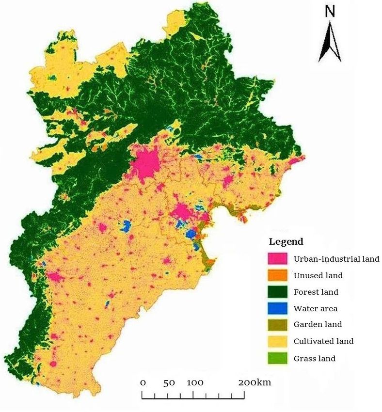
Sustainability 2019, 11, 1446                                                                       2 of 23

population, urban land supply is under increasing pressure. The land resource supply has become an
important factor restricting urban development [1,2]. For most cities around the world, urban sprawl
is becoming the main way to ease urban land tensions. However, the side effects of urban sprawl,
including cultivated land reduction, traffic congestion, and environmental pollution, have further
limited urban development [3–5]. The most reasonable approach for urban sustainable development is
to optimize urban spaces and improve land use efficiency (efficiency is usually defined as output in
relation to input, and land use efficiency is used to calculate the Gross Domestic Product (GDP) per
square meter [6,7]), in addition to making urban land more functional [8,9].
     According to the Code for Classification of Urban Land Use and Planning Standards of Development Land
(GB 50137–2011) [10], urban construction land (the generic name for residential land, public facilities
land, industrial land, storage land, diplomatic land, road plaza land, municipal public facilities land,
green space, and other special land) can be subdivided into multiple categories. Research on specific
urban construction land prediction is increasing gradually. Nevertheless, a comprehensive study
predicting the total urban construction land and specific urban construction land is yet to be carried
out. Moreover, the research methods and content regarding specific urban construction land prediction
need to be improved. Urban–industrial land is the main type of urban construction land [11,12],
and is also the main space for urban non-agricultural activities [13]. China has experienced urban
land expansion alongside rapid urbanization. There was 38.59 million hectares of construction land
by the end of 2015, including 31.42 million hectares of urban-industrial land and rural residential
area. Accounting for 37.4% of the total land supply in China, land supply in the eastern region has
reached an annual increasing rate of 3.9%. There is an increasing pressure on urban land supply [14].
In order to adapt to the new normal of economic development, optimize the land supply structure,
support new industry development, and ensure the rational and healthy development of industrial
land, China has issued a series of policy documents on industrial structure optimization. In October
2015, the Chinese government put forward the development concept of “innovation, coordination,
green development, opening up, and sharing,” clearly aiming to shape the new patterns of regional
coordinated development. Beijing, Tianjin, and Hebei have been required to plan industrial land as
a whole, and control sprawling of urban-industrial land [15]. It is of great significance to explore
urban-industrial land efficiency.
     Meanwhile, China has improved the status of highway traffic through a series of measures
since 2003. The investment in highway and waterway infrastructure had reached 0.23 trillion dollars
by the end of the year 2003. Meanwhile, highway mileage increased by 8260 km, and rural road
mileage increased by 210,000 km [16]. Rapid development to manage highway traffic has effectively
alleviated the tense situation of transportation in China. However, the planning and construction
of the existing national highway network still faced some problems [17]. First, the coverage of the
national highway network was not comprehensive [18]. More than 900 counties across the country
did not have access to national highways, and 18 new cities with populations of more than 200,000,
along with 29 administrative centers at the prefectural level, had not been connected to the national
highways [19]. Second, the transportation capacity is insufficient. The traffic capacity of some highway
channels is tight, and the traffic congestion is serious, which does not meet the needs of rapid traffic
growth [20]. Third, the highway network efficiency is relatively low. The route of the national
highway is discontinuous and incomplete, the links between the national highway and other modes
of transportation are inadequate, and the network benefit and efficiency are difficult to bring into
play [21]. Therefore, it is necessary to consider the role of the national highway in guiding regional
spatial distribution, to optimize the network structure of highways in the eastern region, to strengthen
the construction of links between the east and the west in the central region, to expand the coverage
of the national highway in the western region, and to coordinate urban and rural development.
Putting forward the concept of “accessibility”, which refers to the size of the interaction potential
between two geographical nodes in the traffic network, Hansen (1959) proposed that it was not only
related to the spatial and temporal barrier between two nodes, but also their quality and scale, and he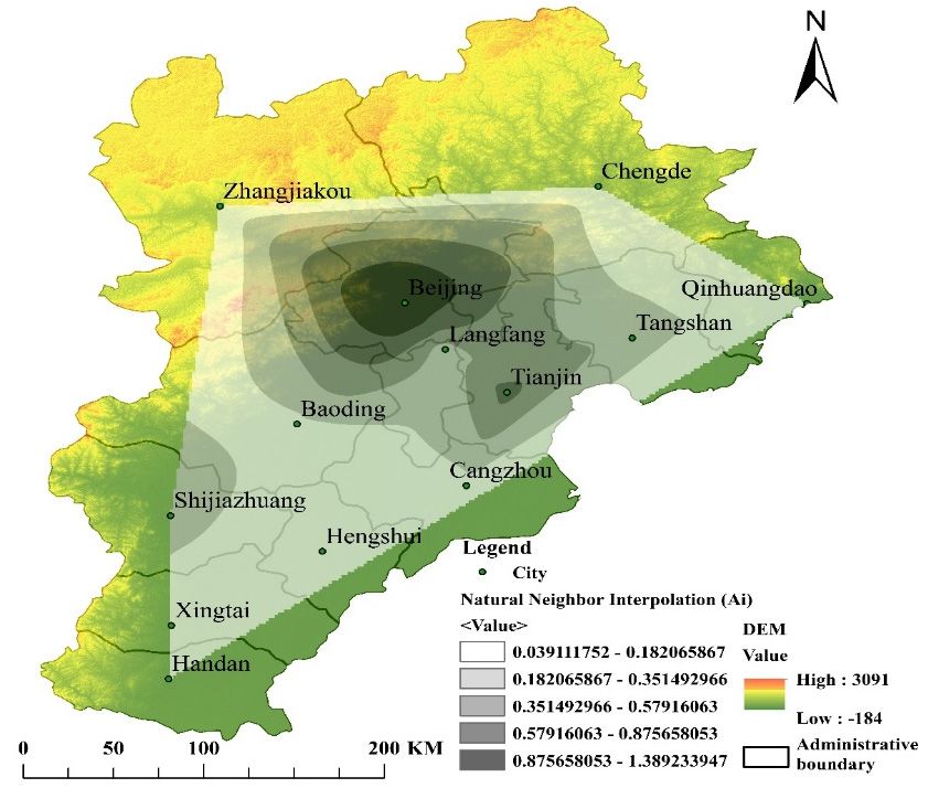
Sustainability 2019, 11, 1446                                                                        3 of 23

studied the relationship between urban land use change and accessibility by using the potential
model. The potential model can be used to calculate the interaction potential between the regional
nodes [22,23]. It is of great necessity to examine in more detail the accessibility of highway networks.
     As one of the emerging economic agglomeration areas in eastern China, many cities in the
Beijing–Tianjin–Hebei (BTH) urban agglomeration have faced problems, such as scattered layouts
and low efficiency of urban-industrial land (their Gross Domestic Product per square meter of
urban-industrial land is low) [24]. Since the implementation of the Beijing, Tianjin, and Hebei
coordinated development strategy in 2014, the industrial transfer projects of Tianjin and Hebei have
blossomed [25]. Tianjin has 15 industrial transfer projects, with a total planning area of 1030 km2 ,
of which only 36.8% (379 km2 ) was in line with the overall land use planning. Meanwhile, 11 cities and
170 counties in Hebei Province have more than 270 industrial transfer projects, with a total planning
area of 19,500 km2 , exceeding the total area of Beijing (16,400 km2 ). The state-owned construction
land supply of Beijing was 4100 ha in 2016, which was 12.2% lower than that in 2015. The industrial
land sales of Tianjin and Hebei also declined from 2015 [26]. Hence, the dilemma between the blind
expansion of undertaking industrial transfer projects and actual demand for land use was obvious.
On the other hand, from the perspective of regional scale, passenger transportation in the BTH area
was heavily dependent on highways, with railways accounting for less than 10% [27]. The public
transit sharing rate in the center of big cities in the BTH urban agglomeration has been increasing over
the past decades. In Beijing, where the public transit share rate was 50%, and the car share rate was
32% in 2015 [27]. Based on the above analysis, transportation integration and industrial upgrading
were the priorities of coordinated development in the BTH urban agglomeration [28].
     For the sustainable development of cities, it is essential to explore the relationship between land
use and urban traffic (traffic in urban areas) from the perspective of spatial layout and traffic planning,
and to analyze the coordination between them. According to the synergy theory between urban
land use and urban traffic, with the continuous coordination development of these two systems,
the relationship between traffic supply and demand could change and a matching mechanism of
supply and demand would be formed [29]. Therefore, this paper aims to examine the coupling
coordination relationship between urban–industrial land use efficiency and accessibility of highway
networks of cities. In specific, in the context of the Beijing–Tianjin–Hebei (BTH) urban agglomeration,
this paper is designed to: (1) examine urban-industrial land use efficiency of BTH cities; (2) estimate
accessibility of highway networks of BTH cities; and (3) identify the coupling coordination relationship
between urban–industrial land use efficiency and accessibility of highway networks.

2. Literature Review
     The interaction between land use and transportation is a hot topic in the fields of geography,
economics, and land use planning [30–35]. Due to the former being a result of urban development,
while the latter is simultaneously an outcome and an important driver, the interaction between urban
land use and transportation is also an interrelated issue in policy making [36–39]. There are two objects
in the evolution of urban land use and transportation: one is housing and enterprise, and the other is
government departments. The location of housing and enterprises determines the distribution of the
population and employment, which constitutes the structure of urban land use. Meanwhile, urban land
use structure affects traffic demand and road investment decisions by the government [40,41]. In recent
years, more and more scholars have been trying to explore the relationship between land use and
urban traffic from the perspective of spatial layout and traffic planning, and to analyze the coordination
between them [42].

2.1. The Effects of Urban Land Use on Urban Traffic
    Urban land use layout plays a decisive role in urban traffic patterns [43]. Many scholars
have proposed that urban land use characteristics have a significant influence on traffic travel
behavior [44]. For example, travel mode, travel distance, and travel distribution could be affected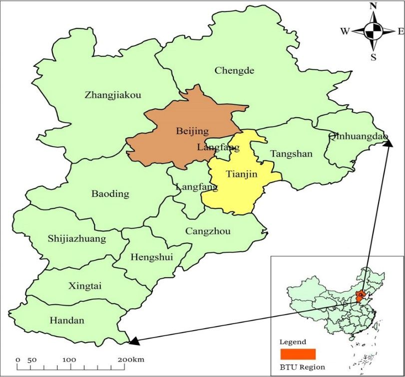
Sustainability 2019, 11, 1446                                                                         4 of 23

by land development density, land use intensity, and land use mixing degree [45,46]. The social,
economic, and ecological efficiency of urban land has formed a relatively mature evaluation system,
and the evaluation objects are basically concentrated in urban construction land [47,48] and industrial
land [49]. The previous research also shows that there are two problems with the evaluation methods of
construction land use efficiency. (1) The relationship between the evaluation indicators and construction
land use efficiency is not correlated closely enough, and the scientific principle of indicator selection
is not reflected [50]. (2) The calculation of comprehensive efficiency is only a summary of the three
aspects of social, economic, and ecological efficiency, and fails to take into account the relationship
between various parts [51,52].

2.2. The Effects of Urban Traffic on Urban Land Use
      The urban transportation network, in affecting the urban land use spatial form, land use intensity,
land use structure, and land price, has promoted the evolution of the urban spatial pattern [53–55].
Land fragmentation caused by the road traffic (traffic on the road) network has shown a significant
spatial correlation with the urban land use spatial form [56]. Meanwhile, attention to the traffic
network, improving location accessibility, and the evolution of the regional land use form along
the route could lead to the formation of new land development intensive areas, and promote the
development of the urban multi-center spatial structure [57,58]. The urban traffic network has shown a
strong spatial attraction effect on land development along its route, and the intensity of land use in the
surrounding areas of the traffic trunk line shows the law of distance attenuation [59]. The influence of
the urban road traffic network on the land use structure is mainly manifested by the spatial attraction
and spatial differentiation effect of traffic lines on urban land evolution [60]. The relevant studies have
revealed the differential effects of different types of traffic corridors, such as light rail, trunk roads
and expressways, on the spatial distribution of residential, commercial, industrial, and other land
in cities [61].
      The research methods of spatial accessibility evaluation mainly include location accessibility,
effectiveness accessibility, and temporal-spatial accessibility [62,63]. The methods of accessibility
evaluation reflect the different research objects: highway [64], expressway [65], subway [66], freight
transport [67], and so forth. Research methods include the distance accessibility model, weighted
average travel time model, time accessibility model, and potential model. The distance accessibility
model, weighted average travel time model, and time accessibility model involve the accessibility
evaluation of the space–time barrier, without analysis of the effect of the main nodal city on the
surrounding nodal cities in an agglomeration area. The interrelationship between cities is not only
related to the level of their own infrastructure, but also to the level of social and economic development,
and the scale of cities in other node cities [68]. Therefore, more and more attention has been paid to the
study of urban accessibility by adding social–economic effects, especially when using the weighted
average travel time model. The weighted average travel time model can be used to measure the time
between a node city and each economic center, through the influence of city size and development
level on accessibility.

2.3. The Interaction between Urban Land Use and Urban Traffic
     Based on accessibility theory and traffic supply and demand equilibrium theory, scholars have
explored the relationship between urban land use and urban traffic. According to accessibility theory,
due to the inhomogeneous distribution of transportation facilities, the difference of accessibility in
different regions directly affects the travel decisions of residents and investment decisions of developers,
thereby affecting land use and development [69,70]. According to traffic supply and demand
equilibrium theory, land use is at the root of urban traffic demand, while the urban transportation
system determines the traffic supply [71]. With the continuous development of the two systems,
the relationship between traffic supply and demand could change, and a matching mechanism of
supply and demand would be formed [72].
Sustainability 2019, 11, 1446 5 of 23
In recent years, scholars have tried to evaluate the coordination of urban land use and traffic
based on various theoretical models (Table 1). The coordination of urban land use and traffic has been
evaluated in terms of the fuzzy- analytic hierarchy process (AHP) multilayer evaluation model [73],
data envelopment analysis model [74], and coupling coordination model [75]. We found that, first,
land use indicators applied fuzzy- analytic hierarchy process (AHP) multilayer evaluation model
focused on residential land area etc. while urban traffic indicators focused on road land area,
etc. Second, land use indicators applied a data envelopment analysis model focused on average
population density, etc. while urban traffic indicators focused on bus passenger capacity, etc. Based
on different models, the land use and urban traffic indicators that have been adopted are diverse.
Moreover, land use indicators applied coupling coordination model focused on land use density, etc.,
while urban traffic indicators focused on length of road network, etc. In addition to this, land use and
public transportation could form an effects and feedback (Coupling Coordination) relationship [76].
Aiming at examining the coupling coordination between urban–industrial land use efficiency and
accessibility of the highway traffic network, the coupling coordination model is appropriate to reveal
the coupling coordination relationships between urban–industrial land use efficiency and accessibility
of highway networks.
Table 1. The evaluation index system of urban land use and urban traffic coordination.
Coordination
Land Use Indicators Urban Traffic Indicators References
Evaluation Model
FUZZY-AHP (Analytic Residential land area, Road land area, public
Hierarchy Process) population density and transport ratio during
[73]
multilayer evaluation employment density, rush hour, vehicle
model land use layout ownership
Average population Bus passenger capacity,
density, area of land for bus share rate, transit
Data envelopment
transport, proportion of mileage, rail transit [74]
analysis (DEA) model
employment and mileage, travel distance
resident population per person
Length of road network,
Coupling coordination Land use density, land length of rail transit
[75]
model use scale, land use layout operation, number of
means of transport
3. Data and Materials
3.1. Study Area
The BTH urban agglomeration, covering a surface area of 217,158 km2 , is an important core
area of northern China, including two municipalities directly under the Central Government of
Beijing and Tianjin, and 11 prefecture-level cities of Hebei Province (including Shijiazhuang, Tangshan,
Qinhuangdao, Handan, Xingtai, Baoding, Zhangjiakou, Chengde, Cangzhou, Langfang, and Hengshui)
(Figure 1). In 2015, the resident population of the BTH urban agglomeration was 110 million, of which
69.573 million lived in cities and towns, and the urbanization rate reached 62.5%. The GDP of the
region was 1.02 trillion dollars, and the proportion of the output value of primary industry, secondary
industry, and tertiary industry was 3.68:40.67:54.67 [77]. There were significant differences in economic
development, industry enterprise development, and road traffic construction in the cities of the BTH
urban agglomeration (Table 2).Sustainability 2019, 11, 1446 6 of 23
Sustainability 2019, 11, x FOR PEER REVIEW 6 of 25
Figure 1.
Figure The map
1. The map of
of the
the BTH
BTH (Beijing–Tianjin–Hebei)
(Beijing–Tianjin–Hebei) urban
urban agglomeration.
agglomeration.
Table 2. Basic information for cities in the BTH (Beijing–Tianjin–Hebei) urban agglomeration.
Table 2. Basic information for cities in the BTH (Beijing–Tianjin–Hebei) urban agglomeration.
Composition of Gross Regional
City
Urban-Industrial
Urban- AreaArea of City Number
of City Numberofof Composition of Gross
Product (%) Regional
2
Land/(km ) Paved Roads Paved Industrial
City Industrial Industrial Product (%)
Roads (ha) Enterprises Primary Secondary Tertiary
Land/(km2) (ha) Enterprises Primary Secondary Tertiary
Beijing
Beijing 1747.33
1747.33 1002910029 3548
3548 0.61
0.61 19.74
19.74 79.7
79.7
Tianjin
Tianjin 1974.67
1974.67 1401914019 5525
5525 1.26
1.26 46.58
46.58 52.2
52.2
Shijiazhuang
Shijiazhuang 586.00
586.00 53665366 2752
2752 9.09
9.09 45.08
45.08 45.8
45.8
Tangshan 1452.00 3098 1595 9.32 55.13 35.6
Tangshan 1452.00 3098 1595 9.32 55.13 35.6
Qinhuangdao 244.00 2137 395 14.21 35.59 50.2
Qinhuangdao
Handan 244.00
454.00 21373161 395
1378 14.21
12.81 35.59
47.16 50.2
40.0
Handan
Xingtai 454.00
354.00 3161 1519 1378
1309 12.81
15.62 47.16
44.97 40.0
39.4
Xingtai
Baoding 354.00
586.00 15193878 1309
1665 15.62
11.78 44.97
50.02 39.4
38.2
Baoding
Zhangjiakou 586.00
456.67 3878 1375 1665
564 11.78
17.87 50.02
40.01 38.2
42.1
Chengde
Zhangjiakou 289.33
456.67 1375 734 549
564 17.34
17.87 46.84
40.01 35.8
42.1
Cangzhou
Chengde 858.67
289.33 734 968 2380
549 9.62
17.34 49.58
46.84 40.8
35.8
Langfang
Cangzhou 363.33
858.67 968 937 1255
2380 8.33
9.62 44.56
49.58 47.1
40.8
Hengshui
Langfang 253.33
363.33 937 742 1234
1255 13.84
8.33 46.15
44.56 40.0
47.1
Hengshui 253.33 742 1234 13.84 46.15 40.0
3.2. Data Collection
3.2. Data Collection
Urban–industrial land use data were collected from the national land utilization conveyance
data Urban–industrial land use data wereAccording
in 2015 (http://www.gscloud.cn/). collected from
to thethe national
overall landland utilization
use plan conveyance
of Beijing, Tianjin,
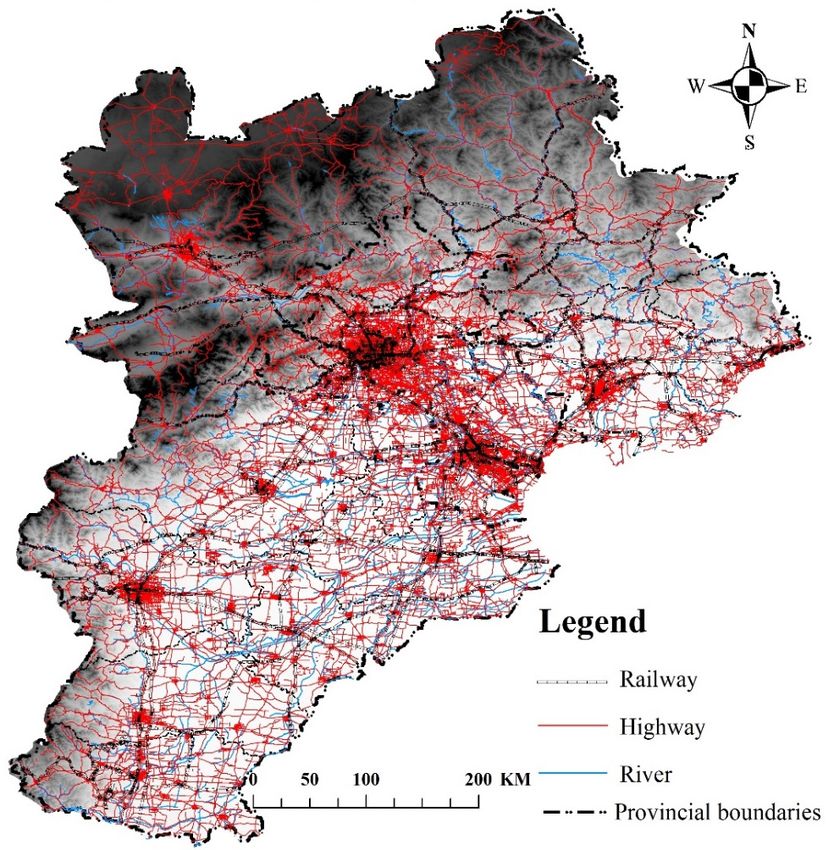
data in 2015 (http://www.gscloud.cn/). According to the overall land use plan of Beijing, Tianjin, andthe year of 2015) of the BTH urban agglomeration, including expressways, urban expressways,
national highways, the local road networks, and administrative boundary, from the Openstreetmap
Database (https://www.openstreetmap.org/). The highway network data set was established by using
the Network Analysis Module in ArcGIS 10.2 (Figure 2b). According to the design speed of the
Highway Engineering Technique Standards (JTG B01-2003) [82], to calculate travel time between the
Sustainability 2019, 11, 1446 7 of 23
discretional nodes of two cities, the average speed of various types of highways was defined:
expressway 100 km/h, urban expressway 80 km/h, national highway 60 km/h, and local road network
40 km/h [82]. Data for the Digital Elevation Model (DEM) was collected from Geospatial Data Cloud
and Hebei, there were significant differences in the total amount of urban–industrial land in different
(http://www.gscloud.cn/).
cities in the BTH urban agglomeration in 2015 (Figure 2a).
Sustainability 2019, 11, x FOR PEER REVIEW 8 of 25
(a)
(b)
FigureFigure 2. (a)
2. (a) Landuse
Land usemap
map of
of the
the (Beijing-Tianjin-Hebei)
(Beijing-Tianjin-Hebei)(BTH) urbanurban
(BTH) agglomeration in 2015; in
agglomeration (b)2015;
highway networks of the BTH urban agglomeration in
(b) highway networks of the BTH urban agglomeration in 2015. 2015.
4. Establishment of the Coupling Coordination Model
4.1. Coupling Coordination Model
Specifically, to quantify the relationships, it is essential to calculate the coupling degree,
coordination degree, and coupling coordination degree in coupling coordination [83].Sustainability 2019, 11, 1446 8 of 23
Statistical data related to socio–economic conditions were collected from the Beijing Statistical
Yearbook 2016 [78], Tianjin Statistical Yearbook 2016 [79], Hebei Statistical Yearbook 2016 [80],
and China Statistical Yearbook for the Regional Economy 2016 [81]. We collected the spatial data
(from the year of 2015) of the BTH urban agglomeration, including expressways, urban expressways,
national highways, the local road networks, and administrative boundary, from the Openstreetmap
Database (https://www.openstreetmap.org/). The highway network data set was established by
using the Network Analysis Module in ArcGIS 10.2 (Figure 2b). According to the design speed of
the Highway Engineering Technique Standards (JTG B01-2003) [82], to calculate travel time between
the discretional nodes of two cities, the average speed of various types of highways was defined:
expressway 100 km/h, urban expressway 80 km/h, national highway 60 km/h, and local road network
40 km/h [82]. Data for the Digital Elevation Model (DEM) was collected from Geospatial Data Cloud
(http://www.gscloud.cn/).
4. Establishment of the Coupling Coordination Model
4.1. Coupling Coordination Model
Specifically, to quantify the relationships, it is essential to calculate the coupling degree,
coordination degree, and coupling coordination degree in coupling coordination [83].
4.1.1. Coupling Degree
The coupling degree literally means the degree of interaction relationships between two
subsystems. It is often adopted to quantify the synergistic effect. The coupling degree model can be
expressed as follows:
1
U1 × U2
k
C=2 (1)
(U1 + U2 ) × (U1 + U2 )
where C denotes the coupling degree, and k represents the adjustment coefficient and is the number
of subsystems, normally set as 2. U1 and U2 stand for the performance levels of the two subsystems
being examined, and the closer the value of U1 or U2 is to 1, the better the performance of the two
subsystems [84]. The value of the coupling coordination degree is always between 0 and 1. When C is
closer to 0, there will be a greater gap between the two subsystems, while a higher C value represents
a higher coupling degree [85]. The coordination status can be divided into four types, namely low
coupling (0 < C ≤ 0.3, meaning the two subsystems have a minimal correlation), antagonism stage
(0.3 < C ≤ 0.5, meaning the two subsystems compete with each other), running-in stage (0.5 < C ≤ 0.8,
meaning the coupling of the two systems is benign), and highly coupling stage (0.8 < C < 1, meaning
that the two systems have a strong correlation) [86].
4.1.2. Coordination Degree
As well as the coupling degree, it is essential to consider the coordination degree, which reflects the
influences of the performance levels of the two subsystems on, or the contributions of the performance
levels, to the coupling coordination degree [87]. The coordination degree can be expressed as follows:
n
T= ∑ β m Um (2)
m =1
where Tj represents the coordination degree, as well as the development level of the system. It can
reflect the extent to which the indicators contribute to the degree of coupling and coordination of the
system [85]. βm represents the undetermined coefficient. Based on previous research [88], we defined
that the contribution of urban–industrial land use efficiency and highway network accessibility to the
whole system are the same. For example, urban–industrial land and the highway network are mutually
improved, but neither are the individual driving factor to each other, so that βm = 0.5 when n = 2.Sustainability 2019, 11, 1446 9 of 23
4.1.3. Coupling Coordination Degree
Although the coupling degree can indicate the interaction relationship between two subsystems,
it is hard to exhibit to what extent the actual development can interact [89]. Therefore, previous
studies have recommended the inclusion of the coupling coordination degree, which is expressed
as [85,87–89]: √
D = C×T (3)
where D represents the coupling coordination degree, and the value belongs to [0,1]. The coupling
coordination degree, reflecting the degree of coupling and coordination of the subsystems during their
interaction, is a positive measurement parameter. Based on previous research, we divided the coupling
coordination degree into ten levels, as shown in Table 3 [85,87].
Table 3. Levels and corresponding criteria of the coupling coordination degree.
Coupling Coordination Type Value Coupling Coordination Level
0.00 < D ≤ 0.09 Extreme imbalance
0.10 ≤ D ≤ 0.19 Serious imbalance
Low coupling coordination
0.20 ≤ D ≤ 0.29 Moderate imbalance
0.30 ≤ D ≤ 0.39 Mild imbalance
0.40 ≤ D ≤ 0.49 Imbalance
Moderate coupling coordination
0.50 ≤ D ≤ 0.59 Coordinate
0.60 ≤ D ≤ 0.69 Basic coordinate
Good coupling coordination
0.70 ≤ D ≤ 0.79 Moderate coordinate
0.80 ≤ D ≤ 0.89 Good coordinate
High quality coupling coordination
0.90 ≤ D < 1.00 High quality coordinate
4.2. Urban-Industrial Land Use Efficiency Evaluation System Design
Urban–industrial land use efficiency refers to the sum of social, economic, and ecological
efficiencies brought to the city through the reasonable arrangement, utilization, and optimization
of urban–industrial land in space and time [14]. Urban-industrial land use efficiency evaluation,
which is the estimation of urban–industrial land structure and function, should not only reflect the
characteristics of urban–industrial land use, but also reflect the function and output of urban-industrial
land [29]. This paper evaluated urban–industrial land use efficiency from three aspects: economic
efficiency, social efficiency, and ecological efficiency. Economic efficiency reflects the relationship
between input and output of land use. Social efficiency reflects the social bearing function, considering
urban–industrial land has effectively supported population agglomeration and public infrastructure
construction. Ecological efficiency is used to measure the impact of urban–industrial land on the
ecological environment.
4.2.1. Data Processing and Weight Determination
In data processing, each indicator was converted by using the extremum method [89].
The calculation processes are expressed in Equations (4) and (5).
Positive indicator:
xij − min x j
x= (4)
max x j − min x j
Negative indicator:
max x j − xij
x= (5)
max x j − min x jSustainability 2019, 11, 1446 10 of 23
where x is the value of indicator xij processed by the extremum method; xij is the actual value of
indicator i in the year j; max(xj ) is the maximum actual value of indicator i in the year j; and min(xj ) is
the minimum actual value of indicator i in the year j.
For weight determination, the coefficient of variation method is used to determine the weight of
each indicator [85]. Determination of the mean value of each indicator’s eigenvalues uses
n
1
xj =
n ∑ xij (i = 1, 2, . . . , n; j = 1, 2, . . . , m) (6)
i =1
where xij represents the eigenvalue of the evaluation object i and the evaluation indicator j; and x j
represents the average of the eigenvalues for item j of all evaluation objects.
Standard deviation determination of the characteristic value of each evaluation indicator uses:
s
1 n
∑
SJ = xij − x j (7)
n i =1
where Sj represents the standard deviation of evaluation indicator j.
Determination of variation coefficient for eigenvalues of each evaluation indicator uses:
Vj = Sj/x j (8)
where Vj represents the variation coefficient for eigenvalues of each evaluation indicator.
Determination of each evaluation indicator’s weight uses:
ω j = Vj/ ∑nj=1 Vj (9)
where ω j represents weight evaluation indicator j.
4.2.2. Urban-Industrial Land Use Efficiency Evaluation
We used a comprehensive evaluation method to evaluate urban–industrial land use efficiency.
The calculation method is given in Equations (10) and (11), as follows:
j
Ei = ∑ Wij × xij0 × 100% (10)
n =1
where Ei represents the single efficiency, and Wij represents the weight of secondary indicators.
3
ESUM = ∑ Wj × Ei × 100% (11)
n =1
where ESUM represents comprehensive efficiency. Wj represents the weight of primary indicators.
4.2.3. Evaluation Indicators
Urban–industrial land is the main component of urban land. The evaluation indicator selection
of urban–industrial land use efficiency should be based on the content of urban land use evaluation,
and according to the particularity of urban–industrial land, the evaluation indicators of urban land
use should be adjusted appropriately. Based on the land use efficiency evaluation system and land
intensive use evaluation system, we selected a range of urban–industrial land use efficiency evaluation
indicators (Table 4).Sustainability 2019, 11, 1446 11 of 23
Table 4. Urban–industrial land use efficiency evaluation system.
Subsystem Index Entropy
Primary Indicators Secondary Indicators
Weight Type Weight
Added value of the second and third
+ 0.0245
industries (14.77 million dollars/km2 ) (U11 )
Economic 0.4586 Average revenue (14.77 million
+ 0.2578
efficiency (U1 ) dollars/km2 ) (U12 )
Average total retail sales of consumer
+ 0.0629
goods (14.77 million dollars/km2 ) (U13 )
Return on fixed assets (%) (U14 ) + 0.1134
Per capita area of urban-industrial land
− 0.0186
(m2 /people) (U21 )
Number of employees in the second and
0.3655 + 0.1438
Social efficiency third industries (10000 people/km2 ) (U22 )
(U2 ) Per capita disposable income of urban
+ 0.0211
residents (dollars) (U23 )
Number of beds per health institution per
+ 0.1764
1000 population (U24 )
Road area per capita (m2 /person) (U25 ) + 0.0057
Green coverage rate of built area (%) (U31 ) + 0.001
Green area rate of built area (%) (U32 ) + 0.0013
0.1758 Energy consumption per unit of industrial
Ecological − 0.1052
output (t/dollars) (U33 )
efficiency (U3 )
Treatment capacity of industrial
+ 0.0002
wastewater (t/km2 ) (U34 )
Treatment capacity of industrial solid waste
+ 0.0681
(t/km2 ) (U35 )
4.3. Accessibility of Highway Networks Evaluation System Design
The accessibility evaluation method proposed in a previous study [21] was used and improved to
evaluate the highway network system (U2 ).
4.3.1. Regional Accessibility Evaluation Method
Various accessibility measurement methods have been employed to calculate different research
objects, such as highways, high-speed railways, subways, and so forth. This paper calculated the time
from a node city to the economic center by using the weighted average travel time model, as well as the
influence of urban scale and development level on accessibility. However, the weighted average travel
time model did not consider the influence of distance decay, and the length of the distance between
the node cities played little role in calculating accessibility. For that reason, studies on accessibility
of the node spatial interaction by using the potential model have become more and more dominant.
Potential, which refers to the force between objects—for instance, the force of j on i Aij is equal to Mj /Cij ,
where Mj refers to the activity scale of node j—is often calculated by a city’s social and economic
development indicators, such as the gross domestic product. Cij refers to the travel impedance factor
(distance). This paper used Ai to show the sum of the forces generated by an object distributed on
objects distributed in space to node i, and the potential model was calculated as follows:
n Mj
Ai = ∑ Cija
(12)
j =1
where a denotes the node cities’ travel friction coefficient, which reflects the influence degree of a
spatial and temporal barrier on the accessibility relation of any two node cities.Sustainability 2019, 11, 1446 12 of 23
4.3.2. Improved Accessibility Evaluation Method
Due to Mj in the method of reachability measurement not reflecting the typicality and
systematisms of indicators selecting, we improved the method by using the city center function
intensity index. The city center function intensity index can reflect the scale of the city and its economic
development level [21]. At first, this paper calculated the function intensity index of every node city’s
social and economic data. Secondly, this paper evaluated the scale of every city, and its economic
development level. The city center function intensity index can be calculated as follows:
Xi
Kx = (13)
(∑in=1 Xi )/n
where Xi refers to the social-economic indicator of city i (the GDP).
This paper used the resident population (Pi ), proportion of urban population (Ui ),
and economically active population (Ei ) to reflect city i’s scale and urbanization level. Then, this paper
calculated the central function intensity indices of the three indicators separately, and denoted them
as KGi , KTi and KVi . To reflect city i’s infrastructural and economic level, this paper selected GDP (Gi ),
the percentage of second industry (Si ), the percentage of tertiary industry (Ti ), and the total investment
in fixed assets (Vi ) as corresponding indices, and denoted them as KGi , KTi and KVi. Due to a lack of
research references regarding indicator selection, this paper had to set identical weights of the center
function index of each indicator to calculate their arithmetic mean value, to obtain every node city’s
scale and economic level index (Mj ), as follows:
K Pj + KUj + KEj + KGj + KSj + KTj + KV j
Mj = (14)
n
Improved potential model:
n
K Pi + KUi + KEi + KGi + KSi + KTi + KVi
Ai = ∑ nCija
(15)
j =1
5. Results and Discussion
5.1. Urban–Industrial Land Use Efficiency
We firstly assessed the urban–industrial land use efficiency, including the economic efficiency,
social efficiency, ecological efficiency, and comprehensive efficiency, of all cities in the BTH urban
agglomeration, as shown in Figure 3.
Overall, there were significant differences among economic, social, and ecological efficiencies,
found through comparing the efficiency values in Figure 3a–c. The economic efficiency of the
urban-industrial land ranged between 0.026 and 0.453, and the social efficiency of the urban–industrial
land of all cities in the BTH urban agglomeration ranged between 0.026 and 0.343. In comparison,
the ecological efficiency of urban–industrial land only ranged between 0.006 and 0.070, far less than
the values of economic and social efficiency. These results are consistent with the long-term city
development pattern in China, in which various local governments have given priority to economic and
social development, while the ecological environment has been neglected. Meanwhile, the low value
of ecological efficiency also reflects that the urban industrial–land in the BTH urban agglomeration is
currently under great ecological pressure, which should be urgently alleviated in future development.
Meanwhile, there were large differences among the economic, social, and ecological efficiencies of
different cities. Obviously, Beijing and Tianjin outperformed other cities in all economic and social
aspects, with economic efficiency values of 0.453 (Beijing) and 0.233 (Tianjin), and social efficiency
values of 0.343 (Beijing) and 0.219 (Tianjin). These values were far higher than those of 11 cities in
Hebei Province. Moreover, Beijing had the highest ecological efficiency value of 0.07, at least twoSustainability 2019, 11, 1446 13 of 23
times the values of all other cities, including Tianjin city. For ecological efficiency, it is observed that
the values of Qinhuangdao and Chengde were much higher, which reflects the preservation of the
ecological environment of these areas during development by local governments. However, other cities
Sustainability 2019, 11, x FOR PEER REVIEW 14 of 25
demonstrated low values. This means Beijing and Tianjin still had the highest urban–industrial land
efficiency, whileassessed
We firstly other cities had low urban–industrial
the urban–industrial land efficiency.
land use efficiency, The the
including apparent
economic differences in
efficiency,
economic, social,ecological
social efficiency, and ecological efficiency
efficiency, have further resulted
and comprehensive in large
efficiency, of all gaps
cities in
in comprehensive
the BTH urban
efficiency (Figure 3d).
agglomeration, as shown in Figure 3.
0.50 0.40
Economic efficiency Social efficiency
0.35
0.40
0.30
0.30 0.25
0.20
0.20 0.15
0.10
0.10
0.05
0.00 0.00
Shijiazhuang
Shijiazhuang
Tianjin
Langfang
Langfang
Tangshan
Handan
Tianjin
Tangshan
Handan
Hengshui
Hengshui
Qinhuangdao
Qinhuangdao
Beijing
Xingtai
Baoding
Zhangjiakou
Chengde
Cangzhou
Beijing
Xingtai
Baoding
Zhangjiakou
Chengde
Cangzhou
(a) (b)
0.08 Ecological efficiency 0.40 Comprehensive efficiency
0.07 0.35
0.06 0.30
0.05 0.25
0.04 0.20
0.03 0.15
0.02 0.10
0.01 0.05
0.00 0.00
Tangshan
Shijiazhuang
Shijiazhuang
Hengshui
Chengde
Tianjin
Beijing
Tangshan
Tianjin
Handan
Baoding
Zhangjiakou
Cangzhou
Langfang
Hengshui
Qinhuangdao
Qinhuangdao
Chengde
Beijing
Baoding
Zhangjiakou
Cangzhou
Langfang
Xingtai
Handan
Xingtai
(c) (d)
Figure3.3.Evaluation
Figure Evaluation results
results of urban-industrial
of urban-industrial land
land use use efficiency
efficiency in the (Beijing–Tianjin–
in the (Beijing–Tianjin–Hebei) BTH
Hebei)agglomeration.
urban BTH urban (a) agglomeration. (a) Economic
Economic efficiency, efficiency,
(b) social efficiency, (b) socialefficiency,
(c) ecological efficiency,
and (c)
(d)
comprehensive efficiency.
ecological efficiency, and (d) comprehensive efficiency.
To understand
Overall, the causes
there were of thedifferences
significant current patterns
amongofeconomic,
urban–industrial landecological
social, and use, we explored the
efficiencies,
economic, social,
found through and ecological
comparing efficiencies
the efficiency based
values on the components
in Figure listed inefficiency
3a–c. The economic Table 4. Undoubtedly,
of the urban-
with advanced manufacturing and modern service industries as pillar industries
industrial land ranged between 0.026 and 0.453, and the social efficiency of the urban–industrial and intensive land
land
use levels,
of all citiesBeijing, Tianjin,
in the BTH urbanShijiazhuang,
agglomeration Qinhuangdao, Tangshan,
ranged between 0.026and
andother
0.343.cities had high levels
In comparison, the
of urban–industrial land use economic efficiencies. Beijing, Tianjin, Baoding, and Langfang
ecological efficiency of urban–industrial land only ranged between 0.006 and 0.070, far less than the showed
high
valueslevels of urban–industrial
of economic and social land use social
efficiency. These efficiencies.
results areBeijing, Qinhuangdao,
consistent Shijiazhuang,
with the long-term city
and Chengde pattern
development showedinhigh levels
China, of urban–industrial
in which land use ecological
various local governments efficiencies.
have given priorityNevertheless,
to economic
due
and to the development,
social particularity of industrial
while industries,
the ecological the ecological
environment environment
has been neglected.in Meanwhile,
Baoding, Tangshan,
the low
Langfang,
value of ecological efficiency also reflects that the urban industrial–land in asthe
and other cities was faced with difficulties in governance. Furthermore, central
BTHcities in
urban
agglomeration is currently under great ecological pressure, which should be urgently alleviated in
future development.
Meanwhile, there were large differences among the economic, social, and ecological efficiencies
of different cities. Obviously, Beijing and Tianjin outperformed other cities in all economic and social
aspects, with economic efficiency values of 0.453 (Beijing) and 0.233 (Tianjin), and social efficiencySustainability 2019, 11, 1446 14 of 23
the BTH urban agglomeration, Beijing, Tianjin, and Shijiazhuang had high levels of urban–industrial
land use comprehensive efficiency.
Overall, in the current era, the advocated pattern of the BTH urban agglomeration is that Beijing
should upgrade its industrial pattern through transferring primary and secondary industry to Tianjin
and cities in Hebei Province [4]. This policy is aimed at conserving land resources, promoting Beijing’s
industry sustainability, and driving the economic and social development of Tianjin and Hebei’s
cities. However, enterprises have only set up subsidiary companies in Tianjin and Hebei’s cities,
without practical operation of these new companies [25]. This, on the one hand, has pulled down the
ecological efficiency of Tianjin and Hebei’s cities, and on the other hand, has significantly deteriorated
the economic and social efficiency of Tianjin and Hebei’s cities without real economic and social output.
However, the current industry upgradation policy of the BTH urban agglomeration has gone astray
because of the imbalance of urban–industrial land use. More critically, the current implementation of
the industry upgradation policy has not only failed to conserve land, but has also severely aggravated
land resource waste [90].
5.2. Accessibility of Highway Networks
Urban economic development affects the spatial direction of traffic flow [91]. By giving economic
weight to the shortest travel time, the weighted average travel time based on time distance can weaken
the spatial blocking effect of geographical location on accessibility, and strengthen the relationship
between economic development and accessibility. Moreover, urban accessibility can be measured
through urban scale and economy [92]. Therefore, measuring the urban scale and economy grade of
the cities in the BTH urban agglomeration, as well as comparing their size and classifying their grades,
is the basic premise for understanding the accessibility of each city. Each node city’s urban scale and
economy grade Mj was calculated using the ArcGIS 10.2 Natural Breaks Classification method, and we
divided the value of Mj into five classes (Table 5). Table 5 presents the urban scale and economy grades
of all cities in the BTH urban agglomeration [93].
Table 5. Urban scale and economy grades of cities in the (Beijing-Tianjin-Hebei) (BTH) urban agglomeration.
Grade Economic Development Characteristics Cities
1 Economic radiation center Beijing, Tianjin
2 Advanced economic agglomeration Shijiazhuang, Tangshan
3 Intermediate economic agglomeration Baoding, Handan
4 Primary economic agglomeration Cangzhou, Langfang, Qinhuangdao, Xingtai, Zhangjiakou
5 Economically backward areas Chengde, Hengshui
As shown in Table 4, there were five types of urban scale and economy grades in the BTH urban
agglomeration, where Beijing and Tianjian were the two cities listed as the economic radiation center.
Among all the cities in Hebei Province, Shijiangzhuang and Tangshan were the two characterized
as having advanced economic agglomeration, with relatively higher urban accessibility, followed by
Baoding and Handan. Cangzhou, Langfang, Qinhuangdao, Xingtai, and Zhangjiakou were cities
with the characteristics of primary economic agglomeration, and Chengde and Hengshui were the
economically backward areas with the lowest urban accessibility.
The highest urban scale and economy grades, which were 3.192 and 2.648 respectively, were shared
by Beijing and Tianjin. Following Beijing and Tianjin, the score of the urban scale and economy grades
of Shijiazhuang and Tangshan, which were important bases for the manufacturing and emerging
industries in the BTH region, were 1.117 and 1.002, respectively. From the regional distribution, as the
top cities of economic development in the BTH region, Beijing and Tianjin shared an urban scale and
economy grade of 1, and were located in the core area of the BTH region. Cities that shared the urban
scale and economy grade of 2, which included Tangshan in the coastal areas and Shijiazhuang in
the west wing, were not only distributed widely, but also showed obvious regional characteristics.
Regional differences indicated that Tangshan and Shijiazhuang have been becoming economic centersSustainability 2019, 11, 1446 15 of 23
of the east and west wings of the BTH region. It was noteworthy that the grade of Cangzhou’s
urban scale and economy was only 4. However, compared with Handan, the resident population
and economically active population of Cangzhou was far less than that in Handan, although their
gross domestic product and percentage of tertiary industry were roughly the same. Therefore, the low
population size has become the restrictive factor of Cangzhou’s urban scale and economy. Baoding
and Handan, whose urban scale and economy grade was 3, were located in the south area of the
BTH region.
The cities that shared an urban scale and economy grade of 4, which included Cangzhou,
Langfang, Qinhuangdao, Xingtai, and Zhangjiakou, were mainly located in the northwest, northeast,
and southeast areas of the BTH region. Cities that shared an urban scale and economy grade of
5, which included Chengde and Hengshui, were mainly located in the north and south areas of
the BTH region. Those cities sharing low urban scale and economy grades were almost always
located in mountainous areas, and their location conditions are very poor. With an urban scale and
economy grade of 5, Hengshui is a barrier to urban agglomeration in the south area, and to core urban
agglomeration in the BTH region. Such a regional difference showed that the radiometric force from
the core urban agglomeration in the BTH region to Xingtai and Handan in the south area was relatively
weak. Generally speaking, spatial differences in urban scale and economy grade characterization
revealed that the farther a city is away from the center of regional economy, the weaker the city’s
external force and economic radiation ability. That is, the urban space and economic radiation ability
between cities was distance diminishing.
We further used the city’s scale and economic level index (Mj ) to reflect the weight index,
and measured the accessibility index (Ai ) of each node city in BTH urban agglomeration, by using the
improved potential model, as shown in Figure 4.
Sustainability 2019, 11, x FOR PEER REVIEW 17 of 25
3.50 1.60
Mj Ai
3.00 1.40
1.20
2.50
1.00
2.00
0.80
1.50 0.60
1.00 0.40
0.50 0.20
0.00 0.00
Shijiazhuang
Hengshui
Langfang
Tianjin
Tangshan
Handan
Qinhuangdao
Chengde
Beijing
Xingtai
Baoding
Cangzhou
Zhangjiakou
Shijiazhuang
Hengshui
Langfang
Tianjin
Tangshan
Handan
Qinhuangdao
Beijing
Xingtai
Baoding
Cangzhou
Zhangjiakou
Chengde
Figure
Figure 4. Accessibility
4. Accessibility indexindex of highway
of highway networks
networks in the
in the BTH BTH (Beijing–Tianjin–Hebei)
(Beijing–Tianjin–Hebei) urban
urban agglomeration.
With a good geographical location and good economic conditions of the surrounding cities, the Ai
of Beijing reached 1.416—optimal in the BTH agglomeration.
region. However, with an urban scale and economy
grade of 4, the Ai of Qinhuangdao (Ai = 0.039) was the lowest in the BTH region. This indicates that
With a good geographical location and good economic conditions of the surrounding cities, the
the greater the distance between the city and the regional economic center, the more obvious the
Ai of Beijing reached 1.416—optimal in the BTH region. However, with an urban scale and economy
influence of geographical location on the level of accessibility. In addition, the Mj and Ai of Baoding
grade of 4, the Ai of Qinhuangdao (Ai = 0.039) was the lowest in the BTH region. This indicates that
and Langfang were heterogeneous. The Ai of Langfang, with an urban scale and economy grade of 4,
the greater the distance between the city and the regional economic center, the more obvious the
was higher than that of Baoding, with an urban scale and economy grade of 3. That the Ai of Baoding
influence of geographical location on the level of accessibility. In addition, the Mj and Ai of Baoding
was slightly higher than that of Handan indicated that the spatial function and economic influence of
and Langfang were heterogeneous. The Ai of Langfang, with an urban scale and economy grade of 4,
the surrounding cities of Langfang were larger than that of the surrounding cities of Baoding.
was higher than that of Baoding, with an urban scale and economy grade of 3. That the Ai of Baoding
was slightly higher than that of Handan indicated that the spatial function and economic influence
of the surrounding cities of Langfang were larger than that of the surrounding cities of Baoding.
Based on the above analysis, using the ArcGIS 10.2 Natural Neighbor Interpolation method, we
obtained the regional accessibility (Ai) spatial pattern and characteristics in the BTH region (Figure
5). From the perspective of geographical location, the Ai of the whole BTH urban agglomeration was
relatively high. The accessibility spatial distribution showed an expanding trend from Beijing toSustainability 2019, 11, 1446 16 of 23
Based on the above analysis, using the ArcGIS 10.2 Natural Neighbor Interpolation method,
we obtained the regional accessibility (Ai ) spatial pattern and characteristics in the BTH region
(Figure 5). From the perspective of geographical location, the Ai of the whole BTH urban agglomeration
was relatively high. The accessibility spatial distribution showed an expanding trend from Beijing to
peripheral cities; namely, the farther a city was away from the center of regional economy, the weaker
the Ai of the city. The geographical location conditions and the city’s urban scale and economy grade
influenced accessibility of the city. The results indicate that the greater the distance between the city
and the regional economic center, the more obvious the influence of geographical location on the level
of accessibility
Sustainability 2019, [93].
11, x FOR PEER REVIEW 18 of 25
5. Regional
Figure 5. Regionalaccessibility
accessibility(A(A
i ) ispatial pattern
) spatial andand
pattern characteristics in the
characteristics inBTH
the (Beijing-Tianjin-Hebei)
BTH (Beijing-Tianjin-
urban agglomeration.
Hebei) urban agglomeration.
5.3. Coupling Coordination Relationship between the Urban–Industrial Land Use Efficiency System and
5.3. CouplingofCoordination
Accessibility Relationship
Highway Networks Systembetween the Urban–Industrial Land Use Efficiency System and
Accessibility of Highway Networks System
Table 5 exhibits the coupling and coordination types between the urban–industrial comprehensive
land Table 5 exhibits
use efficiency and the couplingof and
accessibility coordination
the highway network.types between
Overall, the urban–industrial
the coupling coordination
comprehensive land use efficiency and accessibility of the highway
relationship showed a good coupling degree in Beijing, Tianjin, Qinhuangdao, network. Overall, theLangfang,
coupling
coordination
and Cangzhou. relationship
However, showed a good degree
the coordination coupling degreecities
of these in Beijing, Tianjin,low.
was relatively Qinhuangdao,
The degree
Langfang,
of coupling coordination distinguishes between the benign and the destructive effects of the low.
and Cangzhou. However, the coordination degree of these cities was relatively The
coupling
degree
action. The coordination degree was better than the coupling degree, which indicated that the
of coupling coordination distinguishes between the benign and the destructive effects of the
coupling action. The
urban–industrial landcoordination
use efficiencydegree
system was
andbetter than the of
accessibility coupling
highway degree, which
networks indicated
system werethat
not
the urban–industrial
mutually improved, and landremained
use efficiency system state.
in hysteresis and accessibility of highway networks system were
not mutually
According improved, and remained
to the coupling in hysteresis
and coordination state.
states between the urban–industrial comprehensive
According to the coupling and coordination
land use efficiency (U1 ) and accessibility of the highwaystates between the urban–industrial
network (U2 ), we dividedcomprehensive
the hysteresis
land use efficiency (U 1) and accessibility of the highway network (U2), we divided the hysteresis
statuses of these two systems into three levels: (1) U1 > U2 , urban-industrial land comprehensive
statuses
efficiencyof(Uthese two systems into three levels: (1) U1 > U2, urban-industrial land comprehensive
1 ) hysteresis; (2) U1 < U2 , accessibility of the highway network (U2 ); and (3) U1 = U2 ,
efficiency (U1) hysteresis; (2) U1 < U2, accessibility of the highway network (U2); and (3) U1 = U2,
synchronous development (Table 6). The urban–industrial comprehensive land use level generally
lagged behind the highway network development level in cities of the BTH urban agglomeration,
except in Tangshan.You can also read