Design considerations of photonic lanterns for diffraction-limited spectrometry - Caltech Authors

Research Article Journal of the Optical Society of America B 1

 Design considerations of photonic lanterns for
 diffraction-limited spectrometry
 J ONATHAN L IN , 1,* N EMANJA J OVANOVIC , 2 AND M ICHAEL P.
 F ITZGERALD 1
 1 Physics & Astronomy Department, University of California, Los Angeles (UCLA), 475 Portola Plaza, Los
 Angeles 90095, USA
 2 Department of Astronomy, California Institute of Technology, 1200 E. California Blvd., Pasadena, CA
arXiv:2106.10990v1 [astro-ph.IM] 21 Jun 2021

 91125, USA
 * jon880@astro.ucla.edu

 Abstract: The coupling of large telescopes to astronomical instruments has historically been
 challenging due to the tension between instrument throughput and stability. Light from the
 telescope can either be injected wholesale into the instrument, maintaining high throughput at the
 cost of point-spread function (PSF) stability, or the time-varying components of the light can be
 filtered out with single-mode fibers (SMFs), maintaining instrument stability at the cost of light
 loss. Today, the field of astrophotonics provides a potential resolution to the throughput-stability
 tension in the form of the photonic lantern (PL): a tapered waveguide which can couple a time-
 varying and aberrated PSF into multiple diffraction-limited beams at an efficiency that greatly
 surpasses direct SMF injection. As a result, lantern-fed instruments retain the stability of SMF-fed
 instruments while increasing their throughput. To this end, we present a series of numerical
 simulations characterizing PL performance as a function of lantern geometry, wavelength, and
 wavefront error (WFE), aimed at guiding the design of future diffraction-limited spectrometers.
 These characterizations include a first look at the interaction between PLs and phase-induced
 amplitude apodization (PIAA) optics. We find that Gaussian-mapping beam-shaping optics can
 enhance coupling into 3-port lanterns but offer diminishing gains with larger lanterns. In the -
 and -band (0.97–1.35 μm) region, with moderately high WFE (∼10% Strehl ratio), a 3-port
 lantern in conjunction with beam-shaping optics strikes a good balance between pixel count and
 throughput gains. If pixels are not a constraint, and the flux in each port will be dominated by
 photon noise, then larger port count lanterns will provide further coupling gains due to a greater
 resilience to tip-tilt errors. Finally, we show that lanterns can maintain high operating efficiencies
 over large wavelength bands where the number of guided modes at the lantern entrance drops, if
 care is taken to minimize the attenuation of weakly radiative input modes.

 © 2021 Optical Society of America

 1. Introduction
 The stability of a ground-based spectrometer is primarily limited by atmospheric turbulence, which
 distorts incoming wavefronts and makes the point-spread function (PSF) of an optical system
 temporally unstable. These instabilities can be compounded when aberrated light is transferred
 to an optical fiber if the core diameter of the fiber is large compared to the wavelength of the light.
 Since large-diameter fibers let light propagate in multiple eigenmodes (specifically, the linearly
 polarized or LP modes, which apply for weakly guiding and radially symmetric waveguides [1]),
 the power travelling down these “multi-mode fibers” (MMFs) will continually shift between the
 available modes over the course of propagation, due to bends, imperfections, stresses, and strains
 along the fiber. This is termed modal noise [2,3]. While the issue of modal noise has been partially
 circumvented in the past by scrambling the propagating light with fiber agitators [4], in many cases
 spectrometers fed with single-mode fibers (SMFs) are becoming the more attractive option. SMFs
 have only a single mode of propagation (LP01 ) which automatically eliminates modal noise and

Research Article Journal of the Optical Society of America B 2

 transition zone output end

 lead-in length
 input end

entrance dia. jacket
 cladding
 core

 Fig. 1. The photonic lantern, a tapered waveguide that can adiabatically transfer light
 from a multi-mode fiber-like input end into multiple single-mode cores. In particular,
 the lanterns considered in this work have output geometries similar to multi-core fibers.
 We choose this architecture for simplicity, and neglect propagation in the single-mode
 cores after the lantern transition. For the purpose of this work we additionally assume a
 linear tapering profile between the “lead-in” portion of the waveguide and the lantern’s
 output, along with a core-cladding index contrast of 8.8 × 10−3 and a cladding-jacket
 contrast of 5.5 × 10−3 . Important geometrical considerations in lantern design include
 the lead-in length and taper factor (the degree by which SMF cores shrink from output
 to input).

provides a static beam profile for the spectrometer even in the presence of a temporally fluctuating
input field distribution, greatly improving instrument precision. Diffraction-limited SMF-fed
spectrometers are also significantly more compact than traditional seeing-limited spectrometers,
reducing cost and improving stability against thermal and mechanical deflections [5, 6]. These
gains come at the expense of instrument throughput. Because the LP01 mode is flat in phase and
Gaussian-like in amplitude, efficient coupling into SMFs is difficult at ground-based observato-
ries, resulting in greater light losses in SMF-based fiber injectors over MMF-based fiber injectors.

There are several pathways to increasing throughput while maintaining instrument stability. In
SMF coupling, the first hurdle to overcome is the illumination mismatch between the Airy
pattern of the telescope beam and the Gaussian-like distribution of the fiber mode. One method
to overcome this is by using phase-induced amplitude apodization (PIAA) optics [7]. PIAA
optics use a pair of lenses (or mirrors) in collimated space to reshape the flat-topped aperture
illumination profile of incoming waves into a distribution more amenable for applications such as
fiber injection and coronagraphy. In the context of SMF injection, incoming waves are typically
reshaped to be Gaussian in amplitude, thereby preventing the formation of diffraction rings in
the focal plane. This, in turn, promotes a PSF that better matches the fundamental mode of an
SMF, increasing coupling efficiency. Such “beam-shaping" optics have been shown to work well
(e.g. [8, 9], on SCExAO and KPIC respectively). However, PIAA optics only correct for errors in
field amplitude, not phase. Phase errors (formed from both atmospheric and instrumental effects)
are the second hurdle in efficient SMF coupling. Such errors can be corrected with adaptive optics
(AO), but these systems are less effective at shorter wavelengths. For example, at the short end of
the near-infrared (NIR) and bands (0.97–1.35 μm), where the Strehl ratio (the ratio between
the peak intensity of an aberrated PSF and the peak intensity of an unaberrated PSF) is low
(< 50%), residual phase errors will limit the coupling to < 50%. These wavelength regimes will
be the focus for the next push in direct exoplanet spectroscopy with upcoming instruments such
as HISPEC and MODHIS [10]. An alternative approach is to initially couple aberrated telescope
light into a MMF, which can more efficiently accept light from the complex speckle patterns

Research Article Journal of the Optical Society of America B 3

 Science target

 Spectrometer

 Telescope
 A
 da
 pt

 SMFs
 iv
 e
 op

 Photonic lantern
 tic

 PIAA
 s

 Fig. 2. A diagram of a fiber-fed diffraction-limited spectrometer coupled to a telescope
 with an AO system and a PL fiber injector. The amplitude-remapping effect of PIAA
 optics is shown through gradients, in yellow.

characteristic of low Strehl beams, and “stabilize" the light before injection into the instrument.
The field of astrophotonics makes such a pathway possible via the photonic lantern (PL) [11, 12].
The PL is a waveguide that transitions adiabatically from an MMF-like geometry to a multi-core
fiber (MCF) geometry, allowing light to move between the MMF-like and MCF-like ends with
low loss. Such devices can be formed by heating and tapering one end of either an MCF or a
bundle of SMFs (though methods such as laser inscription can also be used [13], for a review of
construction methods see [12]). A diagram of a PL formed from a tapered MCF is shown in Fig. 1.
Such devices are already in use with fiber Bragg gratings (e.g. GNOSIS [14], PRAXIS [15])
and are currently being considered for use in focal plane wavefront sensing [16, 17]. Figure 2
shows how a PL might be used in the context of high-resolution spectrometry. AO-corrected
(and potentially beam-shaped) telescope light is injected into the MMF-like end of a PL; over
the course of propagation through the lantern, this light becomes efficiently confined within the
single-mode lantern cores, which can then be routed into the science instrument through SMFs.
As such, lantern-based fiber injectors retain both the gain in input coupling efficiency offered
by MMF-based injectors as well as the gain in instrument stability offered by SMF-based injectors.

In recent years, significant headway has been made in our understanding of PLs and their
potential uses in astronomy [16, 18–20]. PLs are also currently being considered for a number of
applications outside astronomy, including mode-selective fiber lasers [21] and amplifiers [22],
spatial mode control in optical fibers [23], LIDAR systems [24], optical ground receivers for
laser satellite communications [25], and free space optical communications [24]. The latter three
investigate how PLs can couple light through the atmosphere, similar to what we consider in
astronomy. This work aims at extending existing studies of PLs to the realm of high-resolution
spectrometry. In particular, we focus on characterizing the chromatic behavior of PLs, their
coupling as function of Strehl, and their performance in the few-port regime (especially relevant
for high-resolution spectrometry which requires many pixels): all properties that must be better
understood before lanterns can make their way into the next generation of spectrometers. To
this end, we present a numerical model for PL performance, as outlined in §2. We then apply

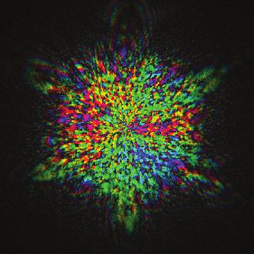
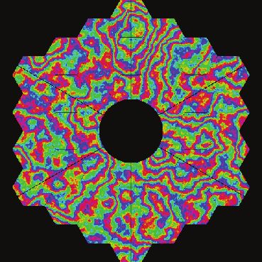
Research Article Journal of the Optical Society of America B 4

this model in §3 to showcase the potential gains offered by PLs across a range of geometries,
wavelengths, and wavefront errors (WFEs), with the aim of informing the next generation of
instrument designs. In the process, we include a first look at the interaction between PLs and
beam-shaping PIAA optics. Results are discussed in §4.

2. Methodology
On-sky testing with an experimental setup is the ultimate way to determine the true performance of
a lantern-based injector. However, before investing in the development of complex infrastructure,
it is important to understand the expected performance with a detailed model; such models will
also help interpret future experimental results. We present a model for lantern performance based
on the statistical assessment of the scalar electric fields at the lantern’s input and output. From
these fields, we compute our prioritized metric for lantern performance: the lantern throughput,
defined as the ratio between total power in the single-mode cores at the lantern’s output and the
total incident power at the lantern’s input (though other metrics, such as the degree of mutual
coherence between the lantern output cores, may also be applicable in other contexts). The
electric field at the lantern’s input is a result of partially compensated aberrations as well as
potential beam shaping, while the output electric field depends on the propagation through the
lantern device.

There are multiple approaches to computing lantern throughput. The electric field distribution
at the lantern output after beam propagation can be readily converted to a lantern throughput,
via overlap integrals (note that this is different than taking the total power of the output field,
which may include extra power in the cladding, not guided by the SMF cores). However, under
certain circumstances, throughput can also be computed from a “modal analysis" perspective
through careful comparison between the input field and the propagating modes of the lantern.
We take both approaches in this work. In this section, we detail our models for WFE (§2.1), AO
correction (§2.2), beam shaping (§2.3), and injection into and propagation through a PL (§2.4).

2.1. Wavefront error
To compute a coupling efficiency for any sort of fiber injector, we first need a statistical model
describing the WFE of light entering our optical system. To this end we assume the standard
Kolmogorov turbulence model for a single thin layer of frozen-flow turbulence translating at a
velocity of 10 m/s. Realizations of turbulent phase screens are generated over a period of 10
seconds, corresponding to 10 pupil crossings over the course of a simulation for an assumed 10
meter aperture. The atmospheric coherence length is a parameter of the simulation, which we
use to adjust the average Strehl ratio of the PSF delivered by the AO correction. Our particular
implementation of Kolmogorov turbulence employs the Fourier-based autoregressive algorithm
of [26]; an example aberrated wavefront in the pupil plane generated with this method is shown
in Fig. 3a. However, Fourier-based turbulence models typically under-represent low-order
WFEs [27]. Additionally, the Kolmogorov power spectrum does not account for other sources
of low-order error such as non-common path aberrations (NCPAs) and mechanical vibrations.
As such, extra low-order phase errors can be added to make WFE more realistic. In this work,
we allow for the injection of extra tip-tilt error by applying a Gaussian-distributed random
displacement to the PSF in the waveguide input focal plane. The magnitude of this displacement
is a parameter of the simulation that can be adjusted. Static WFEs, such as those caused by
misalignment or imperfect optical prescriptions (giving rise to, say, coma or astigmatism), are
neglected.

Research Article Journal of the Optical Society of America B 5

Phase log10(Intensity)
 2π 0
 a b c
3π/2 ‒1

 π ‒2

 Airy ring
π/2 ‒3

 0 ‒4
 d e f

 LP01 LP11 LP02 LP21 LP31 LP12

 g
 LP41 LP03 LP22 LP51 LP32

 Fig. 3. a: the Keck pupil, with turbulence-induced phase errors plotted in color. b:
 the PSF in the absence of WFE. c: same as b but with WFE (∼10% Strehl). d: same
 thing as a, after beam-shaping to a Gaussian illumination profile. e: same thing as
 b, but with beam-shaping. Note the disappearance of the Airy ring. f: Same as c,
 but with beam-shaping. g: The first 19 LP (linearly polarized) modes, the basis for
 propagation down a circular, weakly-guiding step-index fiber. Modes are presented in
 the order they appear as core diameter scales up. Note that all modes with ≠ 0 can
 be rotated by 90◦ to yield another linearly independent mode; these rotations are not
 shown. Modes that appear simultaneously are shown connected. Panels a, d, and g
 display phase information according to the left color bar while panels b, c, e, and f
 display intensity information according to the right color bar.

Research Article Journal of the Optical Society of America B 6

2.2. Adaptive optics
The turbulence-aberrated wavefronts as simulated above are partially corrected using an AO
model built with HCIPy [28], a high-contrast imaging package written for Python. The general
trends in our results will be independent of pupil geometry, but for the purpose of this work we
assume the Keck pupil. We assume a deformable mirror (DM) with 30 × 30 actuators across
the pupil, in line with current “extreme AO” systems and similar to the ∼1,000-element DM
which will be introduced to Keck as part of the phase II of the KPIC project [29]. The control
law is handled using a basic leaky-integrator scheme. Propagation from the pupil to focal plane
is accomplished using HCIPy’s Fraunhofer propagator. Example PSFs from our model in the
presence and absence of turbulence-induced WFE are shown in Figs. 3b and 3c. Finally, for
each tested lantern entrance diameter, we adjust the focal ratio of the optical system in order to
maximize the spatial overlap between the PSF and the lantern modes, ensuring optimal coupling
efficiency.

2.3. Beam-shaping (PIAA) optics
PIAA optics remap the amplitude distribution of light in the pupil plane, in order to promote
a more amenable amplitude distribution (e.g. for fiber injection or coronagraphy) in the focal
plane. This remapping is usually accomplished by a pair of lenses (or mirrors) placed after the
wavefront corrector. In the context of SMF injection, the target amplitude distribution is usually
selected to follow a truncated, circularly symmetric Gaussian profile. This profile removes the
Airy ring, created by diffraction from the pupil mask, and promotes a Gaussian-like PSF that
matches well with the Gaussian-like fundamental mode of SMFs ( [8]; also see the first panel
of Fig. 3g for an example of the fundamental mode). The action of such beam-shaping optics
is shown in the second row of Fig. 3: Fig. 3d shows the Keck pupil post-apodization, while
Figs. 3e and 3f show apodized PSFs with and without turbulence-induced aberrations. Without
beam-shaping optics, coupling efficiencies into SMFs for optical systems with Keck-like pupils
(secondary obstruction ratio of ∼30%) would be limited to ∼65%; with such optics, coupling
efficiencies can reach upwards of 80% [8, 9]. In this work we consider how these optics may also
be applied to lantern-based fiber injectors. We computed the required lens profiles corresponding
to the desired Gaussian amplitude distribution by numerically solving a differential equation for
the lens surfaces, obtained in the geometric optics limit [7]. When we use beam-shaping optics
in our simulations, we propagate wavefronts through lenses with the derived lens profiles, after
correction from the DM but before propagation to the focal plane. For free-space propagation
between the two lenses, we use HCIPy’s angular spectrum propagator.

2.4. Photonic lantern
After propagation to the focal plane, light is injected into a PL. In this work, we only consider
simple lanterns of the type shown in Fig. 1, where the transverse structure of the transition zone
at any point along its length is just a linearly scaled-down version of the lantern’s output (i.e.
isolated single-mode cores in a common cladding). The scale difference between the output
and input ends we term the “taper factor”. Such lanterns deviate slightly from real lanterns in
that the claddings of real lanterns do not necessarily maintain circularity as they taper down;
however, they are a good first approximation. Due to the construction method, lanterns formed
by tapering fibers or fiber bundles may also have a “lead-in” length of MMF-like waveguide at
their input end, which we simulate in our model by extending the tapered end of the transition zone.

The most straightforward way to simulate lantern throughput is to numerically propagate
injected light through the lantern and compute the power in the output lantern modes. However,
numerical propagation is computationally expensive. This expense is multiplied in the presence
of stochastic processes such as turbulence, where numerical propagation must be repeated

Research Article Journal of the Optical Society of America B 7

for multiple realizations of the input electric field in order to obtain a statistical average, and
additionally compounded during parameter space explorations (e.g. over WFE or wavelength,
as done in this work). To simplify and accelerate our simulations, we split throughput into two
parts: coupling efficiency, which reflects the initial loss of light during coupling into the lantern
entrance, and transition efficiency, which reflects losses that occur during propagation through the
lantern. Previous works have shown that transition efficiencies can be as high as ∼97% [11, 30];
a necessary but insufficient condition for this to occur is to have at least as many single-mode
outputs (or “ports") at the lantern exit as guided modes at the lantern entrance [12]. Assuming
negligible transition effects, the input coupling efficiency of the lantern can be taken as a proxy
for overall lantern throughput, bypassing the need to simulate the lantern transition and saving on
computation time. In this work, lantern coupling efficiencies are generally computed under the as-
sumption that the number of ports equals the number of modes and transition losses are negligible.

Coupling efficiencies on their own are quick to simulate. We only need to compute a ba-
sis of “lantern modes”: a set of orthogonal, linearly independent field distributions at the lantern
entrance which span the space of bound electric field distributions when propagated to the lantern
output. Then, the coupling efficiency into a lantern entrance for a given input electric field is
simply the total amount of power coupled into all of the lantern modes, which we can compute
via overlap integrals between the input field and the lantern modes. The overlap integral for
two scalar complex fields 1 and 2 is given by
 ∫ 2
 1∗ 2 
 = ∫ ∫ . (1)
 | 1 | 2 | 2 | 2 

For large lantern taper factors (small residual SMF cores at the lantern’s entrance), the lantern
modes approach the LP modes: analytically known eigenmodes of propagating waves in a
circularly symmetric step-index fiber. Example amplitude distributions for the first 19 LP modes
are shown in Fig. 3g (rotated variants of modes ≠ 0 are not shown).

Later in this work we compute lantern throughputs (rather than input coupling efficiencies),
and extend lantern characterization over regimes where lantern operation has been considered
“inefficient” and the above approach breaks down. In these regimes, we need to apply full
numerical beam propagation to connect the electric field distributions at the lantern input and
output. In order to simulate the propagation of light through PLs, we have built “Lightbeam” [31]:
a numerical package which uses the “finite-differences beam propagation method” (FD-BPM)
algorithm to numerically and implicitly solve the paraxial Helmholtz equation in the weakly
guiding regime. Our particular variant of FD-BPM is based on the algorithm presented in [32],
which is accurate to 4th order transversely, to 2nd order longitudinally, and works on an adaptive
mesh. We have tested this code against RSoft BeamProp, a commercial package for optical
propagation, with consistent results. We have also verified that our code reproduces the expected
behavior for single and few-mode circularly symmetric step-index fibers.

2.5. Tested configurations
All simulated lanterns are assumed to have a fluorine-based glass jacket and a fused silica
cladding with an index contrast of 5.5 × 10−3 , materials typically used to construct lanterns
(private communication with S. Leon-Saval). We consider lantern operation across the as-
tronomical and bands (0.97–1.35 μm), where the Strehl ratio of typical AO systems is
lower and there is a stronger need for PLs. The embedded SMF cores are assumed to have
similar specifications to OFS ClearLite 980 16 fiber, which has a core-cladding index con-
trast of 8.8 × 10−3 and a nominal core diameter of 4.4 μm. This fiber was chosen due to its

Research Article Journal of the Optical Society of America B 8

single-mode cutoff at 970 nm, consistent with our chosen wavelength range. We additionally as-
sume linear lantern taper profiles throughout this work; other geometric parameters are adjustable.

We use this model to assess lantern performance as a function of entrance diameter, wave-
length, and WFE, as well as the length of the lantern’s lead-in waveguide and taper factor.
We also compare the performance of SMFs and 3-, 6-, and 19-port lanterns with and without
beam-shaping optics. We have chosen to consider 3- and 6- port lanterns because their low port
counts make them more applicable for use in high-resolution spectrometers, which require many
pixels and lack room for many fibers. We additionally consider the 19-port lantern because such
devices are already in use (e.g. GNOSIS [30], PRAXIS [15]). Additionally, these port numbers
were selected because they reflect how the number of guided modes increases as core diameter is
scaled up and/or wavelength is scaled down.

3. Results
In this section, we characterize lantern performance as a function of Strehl ratio, operating
wavelength, and geometric factors including lantern entrance diameter, taper factor, and lead-in
waveguide length. Sections 3.1 through 3.5 characterize lantern performances in terms of
coupling efficiency into the lantern entrance, which serves under most circumstances as a good
proxy for lantern throughput. In Section 3.6, we use full numerical beam propagation to compute
proper throughputs and extend the results of prior sections.

3.1. Coupling efficiency vs. Strehl ratio
With the index contrast of the lantern fixed, the primary factor that governs lantern coupling
efficiency is the diameter of the lantern’s input waveguide, which sets the number of supported
modes at the lantern’s entrance and thus determines the lantern’s ability to accept aberrated
light. We present coupling efficiencies at = 1 μm into the input ends of lanterns for various
entrance diameters (and hence mode counts) as a function of Strehl ratio in Fig. 4a. The Strehl
ratio is computed from the intensity average of 100 turbulence-aberrated PSF realizations. We
additionally adjust focal ratio to maximize the overall coupling efficiency at each core diameter
(re-optimizing the focal ratio when beam-shaping is included in the optical system). We assume
that the embedded SMF cores are small after tapering (large taper factor) and that the lantern
entrance is circular, so that the lantern modes can be taken as the LP modes. Other geometric
parameters such as lead-in length are for now irrelevant; we consider them again in Section
3.6. WFE was solely generated from Fourier-based Kolmogorov turbulence (no extra tip-tilt
was added; we consider extra tip-tilt later in §3.5). Figure 4a indicates that coupling efficiencies
increase linearly with Strehl ratio independent of mode count, with the largest mode count lantern
consistently outperforming all other configurations. Performance gains from PLs over SMFs
are also evident across the entire range of tested Strehl ratios: even at 10% Strehl, the simplest
three-mode lantern outperforms direct injection into an SMF by a factor of 2, netting a throughput
of ∼10%. In the absence of beam-shaping optics, six-mode lanterns offer even greater gains,
reaching a ∼15% increase over both SMFs and three-port lanterns at 70% Strehl ratio.

3.2. Effect of lantern size
In Fig. 4b, we extend the previous calculation over a range of core diameters, this time fixing
turbulence to give an average 10% Strehl at the operating wavelength of 1 μm. As its diameter
increases, the number of guided modes at the lantern’s entrance increases in a stepwise fashion,
resulting in discontinuous jumps in the lantern coupling efficiency. Importantly, the number of
guided modes (annotated at the bottom of the plot) does not increase one at a time: modes usually
appear in groups of 2 or 3. Figure 4b shows that the most significant gains in coupling efficiency
occur in the 1- to 3-mode transition and the 3- to 6-mode transition at 10% Strehl, beyond which

Research Article Journal of the Optical Society of America B 9

 a b
 0.25
 0.6 with PIAA
Coupling efficiency without PIAA

 Coupling efficiency
 0.20
 0.5

 0.4 0.15

 0.3
 0.10
 0.2
 λ = 1 µm
 1 mode 6 mode Avg. Strehl = 10%
 w/ PIAA w/ PIAA 0.05
 0.1 3 mode 19 mode
 19 21
 w/ PIAA w/ PIAA
 1 mode 3 6 8 10 12 15 17
 0.0 0.00
 10 20 30 40 50 60 70 5.0 7.5 10.0 12.5 15.0 17.5 20.0 22.5
 Strehl ratio (%) Core diameter (µm)

 Fig. 4. a: coupling efficiency comparison for 1-, 3-, 6-, and 19-mode lanterns against
 Strehl ratio at = 1 μm, with and without beam-shaping (PIAA) optics. Lantern
 entrances were approximated as step-index fibers. The specified mode counts were
 selected because they reflect how the number of LP modes increases with core diameter.
 PSF degradation was simulated using standard Kolmogorov turbulence. b: Mean fiber
 coupling efficiency in the presence and absence of beam-shaping optics, at a wavelength
 of 1 μm for an average Strehl ratio of 10%. The number of available LP modes is
 annotated at the bottom.

increases in lantern size and modality yield diminishing returns. However, if the increases in
instrument complexity and exposure times are not a concern, it may still be beneficial to adopt a
high-mode count lanterns: as seen in Fig. 4, the coupling efficiency of a 19-port lantern is around
double that of a 3-port lantern at 10% Strehl.

 a b
 50
 Relative boost from PIAA (%)

 λ = 1 µm 1 mode (4.4 µm) λ = 1 µm
 3 mode (8.0 µm)
 Avg. Strehl = 10%
 40 6 mode (12.4 µm)
 19 mode (21.8 µm)

 30

 20

 10
 19 21
 10 12
 0 1 mode 3 6 8 15 17
 10 20 30 40 50 60 70 5.0 7.5 10.0 12.5 15.0 17.5 20.0 22.5
 Strehl ratio (%) Core diameter (µm)

 Fig. 5. a: relative coupling efficiency boost offered by Gaussian beam shaping optics
 as a function of Strehl ratio, for various lantern entrance diameters. Large lanterns
 show less gain over all tested Strehl ratios. b: relative coupling efficiency boost from
 beam shaping optics as a function of lantern entrance diameter. We approximate the
 lantern entrance as a step-index MMF. As diameter increases, the boost offered by
 beam shaping optics decreases, dropping below 10% in the 6-mode region.

3.3. Effect of beam-shaping (PIAA) optics
Figure 4 shows the absolute coupling gains from beam-shaping optics as a function of Strehl
ratio and lantern entrance diameter. We recast these results in terms of the relative gains

Research Article Journal of the Optical Society of America B 10

offered by beam-shaping optics in Fig. 5. As indicated in panel a, we see that beam shaping
optics offer a significant ∼30% boost to SMF coupling, consistent with results from [8, 9]. We
additionally see that these beam-shaping optics also offer a significant ∼25% boost to coupling
into a 3-port lantern, but offer negligible ∼5% gain for a 6-port lantern. Consequently, we
find that the 3-port PL with beam-shaping performs almost as well as a 6-port lantern over
the entire range of Strehl ratios (see Fig. 4a). Figure 5b makes a similar argument, showing
that as lantern entrance diameter (and the number of supported modes) increases, the relative
boost afforded by beam-shaping optics drops, declining below 5% beyond the 6-mode region,
with negligible gains for lanterns with 10+ ports. The reason for this will be described in Section 4.

The bump in relative boost in the 21-mode region shown in Fig. 5b can be traced to the
LP13 mode, which in the 21-mode region is very close to its cutoff wavelength and thus extends
further into the cladding. This mode shape matches well with the amplitude distribution produced
by our beam-shaping optics; a similar effect can be seen at the beginning of the 3 mode region
in the same figure, where the relative boost initially spikes because the LP11 mode is close to
its cutoff wavelength and thus has a larger spatial extent. Such modes can be more sensitive to
losses (e.g. due to bending [1]) so it is unclear if these coupling gains are realizable or if they are
an artifact of our idealized simulations.

3.4. Chromatic behavior
We extend the results from Fig. 4a over wavelength in Fig. 6, again fixing atmospheric turbulence
to give PSFs with an average 10% Strehl at the nominal operating wavelength of 1 μm. Here,
we fix the number of PL ports to be equal to the number of modes at the PL entrance, at the
reference wavelength = 1 μm. With the exception of the 19-port lantern, this assumption
ensures that the lanterns will have at least as many output ports as entrance modes over the and
J bands. Unsurprisingly, we see from Fig. 6 that configurations with larger lanterns consistently
outperform those with smaller lanterns across the entire range of tested wavelengths. Additionally,
as wavelength increases, phase error decreases, and coupling efficiency into lanterns typically
increases for all entrance diameters, though there are dips and discontinuous drops as the guided
modes at the lantern entrance change shape and eventually disappear. The discontinuous drops in
coupling efficiency seen in Fig. 6 indicate transition wavelengths across which the number of
guided modes at the lantern entrance changes. Importantly, near such wavelengths, we no longer
expect coupling efficiency to be an accurate proxy for lantern throughput. The reasoning is as
follows: as wavelength increases past a transition wavelength, lantern modes at the waveguide
entrance that were originally guiding now become weakly radiative. Normally, we expect that
such modes would not be able to carry power; however, if the characteristic length scale for
radiative attenuation is small compared to the length of the lantern lead-in, losses are negligible
and these radiative modes can still transfer power into the lantern cores. This effect is relatively
unimportant for large lanterns (e.g. a few percent difference in coupling efficiency for the 19-port
lantern in Fig. 6) since such lanterns will distribute power over many modes. However the effect
can be significant for few-mode lanterns. In Section 3.6, we apply numerical beam propagation
to compute throughputs of few-port lanterns in these transition regimes.

3.5. Tip-tilt wavefront error
To make our WFE more realistic, we can inject extra tip-tilt in addition to the existing WFE from
Kolmogorov turbulence. Similar to Fig. 4b, Fig. 7 plots the mean coupling efficiency for a PL as
a function of entrance diameter, though now under varying amounts of injected tip-tilt error. The
focal ratio of the optical system was optimized to match the size of the lantern modes at each
core diameter prior to tip-tilt injection. Scenarios without beam-shaping optics (panel a) and
with such optics (panel b) are considered. The atmospheric coherence length is tuned to give an

Research Article Journal of the Optical Society of America B 11

 0.40
 4.4 µm (1 mode @ λ 0) Strehl = 10% @ λ 0
 0.35 8.0 µm (3 mode @ λ 0)
 12.4 µm (6 mode @ λ 0)
 0.30 21.8 µm (19 mode @ λ 0)

 Coupling efficiency
 0.25
 λ0
 0.20

 0.15

 0.10

 0.05
 y band J band
 0.00
 0.9 1.0 1.1 1.2 1.3 1.4
 Wavelength (µm)

 Fig. 6. Throughput comparisons for the lantern configurations in Fig. 4a, now as a
 function of wavelength. Simulated atmospheric conditions were fixed for an average of
 10% Strehl at = 1 μm. Dotted lines show the coupling efficiencies with beam-shaping
 (PIAA) optics. For each curve, the focal ratio is optimized at the nominal core diameter
 assuming a wavelength of 1 μm.

average 70% Strehl ratio at a wavelength of 1 μm (actual Strehl of the intensity-averaged image,
after tip-tilt injection, will be lower). Figure 7 shows that coupling degrades as both the amount
of injected tip-tilt increases and as entrance diameter decreases, suggesting that the reduction
in coupling performance due to the injected tip-tilt ultimately depends on the relative amount
of tip-tilt displacement compared to the size of the lantern entrance. Coupling appears mostly
unaffected so long as the RMS tip-tilt displacement is smaller than the lantern entrance radius by
more than a factor of 2.

 a b
 1.0
 No PIAA With PIAA 0 µm rms displacement
 Strehl = 70% w/o injected TT 1 µm
 0.8 λ = 1 µm 2 µm
Coupling efficiency

 3 µm
 4 µm
 0.6

 0.4

 0.2
 19 21 19 21
 1 mode 3 6 8 10 12 15 17 1 mode 3 6 8 10 12 15 17
 0.0
 0 5 10 15 20 0 5 10 15 20 25
 Core diameter (µm) Core diameter (µm)

 Fig. 7. Similar to Fig. 4b, but the atmospheric coherence length is fixed to give an average
 Strehl of 70%, after which tip-tilt WFE in the form of random displacements in the
 focal plane is injected to wavefront realizations. This tip-tilt is added with the intention
 to approximate instrumental tip-tilt and compensate for potential underestimation of
 low-order error in our turbulence model.

Research Article Journal of the Optical Society of America B 12

 0.7
 varying tip-tilt, no PIAA
 varying tip-tilt, PIAA
 0.6 varying r0 , no PIAA
 varying r0 , PIAA
 0.5

 Coupling efficiency 0.4

 0.3

 0.2
 Strehl = 70% w/o injected TT
 0.1 8 µm entrance diameter
 λ = 1 µm
 0.0
 0 10 20 30 40 50 60 70 80
 Strehl ratio (%)

 Fig. 8. Coupling efficiency vs Strehl ratio into an 8 μm diameter (3 mode) fiber for
 aberrated PSFs. Aberrations can be introduced in multiple ways; we consider two. In
 the first we assume only single-layer atmospheric turbulence and vary the coherence
 length 0 . In the second we degrade the PSFs by fixing some 0 and then injecting
 additional tip-tilt error in the form of random displacements in the focal plane. In this
 case, we fixed the 0 to give 70% average Strehl before injecting tip-tilt. Both with and
 without beam-shaping (PIAA) optics, MMFs are better able to capture light degraded
 via the second method.

We present an alternative perspective on lantern performance in the presence of tip-tilt in
Fig. 8, comparing coupling efficiency against Strehl ratio for a lantern entrance diameter of 8
μm in two distinct cases: either tuning Strehl by adjusting atmospheric coherence length or
by adjusting the RMS displacement of injected tip-tilt error. Figure 8 indicates that coupling
efficiencies are comparatively better in the latter case, implying that few-mode fibers and PLs are
resilient against tip and tilt: for a given amount of WFE, coupling efficiency of the beam into the
fiber or lantern improves when there is more power in tip-tilt aberrations vs pure Kolmogorov
turbulence. This holds whether or not beam-shaping optics are used. With this in mind, we see
that the results of §3.1-§3.4 and later §3.6, which do not include additional tip-tilt, are lower
bounds on the coupling gains that can be realized by lanterns in real optical systems. The degree
of this effect will depend on lantern size and the specific characteristics of instrumental tip-tilt.

3.6. Full beam propagation
Because beam propagation is more computationally expensive than the prior coupling calculations,
we apply this method only to study the simplest 3-port lantern; the general trends from this
section will be extensible to larger lanterns. Figure 9 presents the throughput (not input coupling
efficiency) for a 3-port lantern with an 8 μm entrance diameter with beam-shaping optics (black
curve). In throughput calculations, geometric factors such as lead-in length and taper factor
now become relevant; we assume a 4× taper factor, and no lead-in waveguide. To generate the
throughput curve in Fig. 9, we have numerically computed the lantern modes at the waveguide
entrance by backpropagating the fundamental modes of the SMF cores from the lantern output
and orthogonalizing the resulting basis. These modes are LP-like, but will no longer necessarily
be guiding within the lantern entrance if there are more lantern cores than propagating modes at
the lantern’s MMF-like input. Calculation of the lantern modes allows us to retain our modal

Research Article Journal of the Optical Society of America B 13

analysis approach and compute lantern throughput from the input electric field distribution at
the lantern entrance. As a result, we bypass the need to forward-propagate multiple realizations
of the input field through the guide, saving on computation time. As seen in Fig. 9, lantern
throughput agrees well with the coupling efficiency into a similarly sized step-index fiber until
the propagating wavelength approaches the 3 → 1 mode transition wavelength at ∼ 1.32 μm.
Beyond 1.32 μm, the lantern throughput exceeds step-index fiber coupling efficiency by almost a
factor of 2. This is because an 8 μm diameter step-index fiber with our assumed core and cladding
materials becomes single-mode beyond = 1.3 μm; however, an 8 μm diameter lantern entrance
retains weakly attenuating radiative modes which can help transfer power to the lantern cores.

 0.40
 MMF coupling
 0.35 no lead-in
 0.01 cm lead-in
 Lantern throughput

 0.30 0.1 cm lead-in
 1 cm lead-in
 0.25

 0.20

 0.15

 0.10
 3 to 1 mode transition
 0.05
 y band J band
 0.00
 0.9 1.0 1.1 1.2 1.3 1.4
 Wavelength (µm)
 Fig. 9. Throughput of an 8 μm diameter lantern against wavelength, for various lantern
 lead-in lengths. WFE here is wholly generated from Kolmogorov turbulence with
 an average 10% Strehl. The dotted curve denotes coupling efficiency into an 8 μm
 diameter circular step-index fiber; all other curves denote lantern coupling efficiencies
 and were generated using beam propagation. Beyond 1.32 μm, the step-index fiber
 becomes single-mode, and coupling efficiency drops precipitously. However lanterns
 with short lead-in lengths do not experience such a drop due to radiative modes. Note
 that throughputs for non-zero lead-in lengths were only computed and plotted for
 > 1.26 μm to save on computation time.

As such, over transition wavelengths where radiative lantern modes are active, the length
of the lead-in waveguide becomes a relevant factor in lantern design. To show this effect, Fig. 9
plots throughput curves for lanterns that are similar to our 3-port configuration with the exception
of differing lead-in lengths (note these throughputs were only computed for > 1.26 μm to
save on computation time). Throughputs are now computed using the “brute-force” method of
numerically propagating all input field realizations to the lantern’s output. Note that we can no
longer use backpropagation when attenuation through the lantern is non-negligible (as can be the
case for lead-in waveguides): the departure of light from the simulation zone makes the operation
of numerical propagation non-invertible. Figure 9 verifies that longer lead-in lengths result in
greater dampening in lantern throughput at wavelengths beyond the transition wavelength of 1.32
μm, due to increased attenuation of the radiative modes (note that this attenuation is being captured
by the numerical beam propagation itself, not some assumed fiber model). The magnitude of at-

Research Article Journal of the Optical Society of America B 14

tenuation also increases as the propagation wavelength increases beyond the transition wavelength.

The reduction in throughput due to attenuation of the radiative modes will also depend on
the lantern taper factor, which sets the degree by which the embedded SMF cores in the lantern
shrink from output to input. Figure 10 plots the degree of attenuation for the LP11 -like radiative
mode in the lead-in waveguide of a 3-mode (8 μm entrance diameter) lantern, as a function of
taper factor ; since the SMF cores at the output end of the lantern are 4.4 μm in diameter, the
diameter of the tapered-down cores embedded in this lead-in waveguide can be computed as
4.4 μm / . The propagation wavelength is taken to be 1.4 μm. Attenuation is quantified in terms
of the attenuation length , the distance over which power in the radiative mode drops by a factor
of . The attenuation length can be computed from
 
 = (2)
 4 Im ( eff )
where eff is the (complex) effective index of refraction for the radiative mode and Im denotes
taking the imaginary part. In turn, we compute the effective index using FemSIM [33], a
finite-element mode solver that can compute the effective indices of radiative modes. From
Fig. 10, we see that the attenuation of this radiative mode increases as taper factor decreases and
the embedded SMF cores at the lantern entrance become larger. The dependence between the
attenuation length and taper factor is asymptotic, climbing rapidly to infinity as the embedded
SMF cores at the lantern’s entrance approach the minimum required size to become guiding.
Finally, we note from Fig. 10 that the attenuation length for a 3-port lantern with a taper factor of
4 is ∼3 cm. This is order-of-magnitude consistent with Fig. 9, computed using our numerical
beam propagator, where we see that the 3-port, 4× tapered lantern begins to show significant
attenuation at = 1.4 μm when the lead-in length reaches 1 cm.

4. Discussion/Future directions
Our results from Fig. 4a recover the linearly increasing trend of coupling efficiency with Strehl
ratio, consistent with prior works [8]. This is sensible: the Strehl ratio is directly proportional
to peak PSF intensity, which in turn is directly proportional to the amount of PSF power that
couples into the lantern modes. The coupling boost provided by the beam-shaping optics also
increases with Strehl ratio, since beam-shaping optics only correct for average pupil illumination
and not WFE. The boost is greatest for SMFs, which in conjunction with beam-shaping actually
approach the performance of 6-port lanterns at high Strehl. This behavior is expected: at high
Strehl, beam-shaping moves the bulk of light at the focal plane into the PSF core, promoting
coupling into the single Gaussian-like mode of SMFs. In contrast, larger lanterns have access to
other higher-order modes which can couple light away from the PSF core, such as light in the
Airy rings, reducing the utility of beam-shaping. In the case of the 6-port lantern, the presence
of the LP02 mode allows such lanterns to efficiently couple light from the Airy ring. However,
in the low-Strehl regime PLs are still preferable. This result is reaffirmed in the presence of
increased tip-tilt error: the extra size and modality of lanterns makes their coupling efficiencies
less sensitive to displacement of the PSF core. In fact, Fig. 8 shows that for tip-tilt-varied WFE,
lantern coupling efficiency scales roughly with the square root of the Strehl ratio. In contrast,
coupling scales linearly with Strehl when WFE is purely generated from AO-filtered Kolmogorov
turbulence.

Unsurprisingly, we also find that larger lanterns couple more light than smaller lanterns at
a given Strehl ratio, because the number of supported modes increases with lantern entrance
diameter. However, in the absence of beam-shaping, we show in Fig. 6 that gains from increasing
lantern size begin to diminish beyond the 6-port lantern: the absolute coupling gain from a 6- to a

Research Article Journal of the Optical Society of America B 15

 λ = 1.4 µm
 20 8 µm dia.

 Attenuation length (cm)
 10

 5
 4
 3

 2

 Simulation MCF SMF
 1
 1 2 3 4 5 10 20 30
 Tapering factor

 Fig. 10. Attenuation strength vs. taper factor for one of the radiative LP11 -like modes
 ( = 1.4 μm) in a lead-in waveguide for a 3-port, 8 μm diameter lantern, computed with
 FEMSIM [33]. Attenuation strength is quantified as the length over which the total
 power of the radiative LP11 -like mode drops by a factor of . The required taper factors
 to construct the assumed lantern from a bundle of SMFs (125 μm diameter cladding)
 and a MCF (125 μm diameter cladding overall), as well as the taper factor of the lantern
 simulated in Fig. 9, are annotated with vertical dashed lines.

19-port lantern is roughly the same as the gain from a 3- to a 6-port lantern. This result is reiterated
by Fig. 4b, and stems from the fact that low-order modes such as LP01 , LP11 , and LP02 play a
larger role in accepting injected light than higher-order modes, especially when WFE is dominated
by low-order aberrations. The LP11 modes are well-suited for dealing with tip-tilt aberrations,
and account for the increase in coupling efficiency from a SMF to a 3-port lantern. Similarly, in
the absence of beam-shaping, the increase in coupling efficiency from a 3 to 6-port lantern is
primarily due to the inclusion of the LP02 mode (Fig. 3g), which can accept light from the Airy ring.

In the presence of Gaussian beam-shaping optics, diminishing returns begin even sooner:
as seen in Fig. 4a, a 3-port lantern with beam-shaping performs almost as well as a 6-port lantern
with or without beam-shaping. As mentioned above, such lenses have a significant effect for
three-port lanterns (and SMFs) since such devices have no other way to efficiently accept light
from the Airy ring; in contrast, such lenses are less useful for 6-port and larger lanterns, which
have access to the LP02 mode. However, it is important to recognize that these results are specific
to our simple Gaussian-remapping implementation of beam-shaping. Lenses with more advanced
remapping functions, tailored to individual lantern mode geometries and imaging systems, may
boost coupling more and warrant further exploration. Also of interest are optical systems with
two DMs, allowing for simultaneous phase and amplitude modulation without any requirement
for radial symmetry. Careful configuration of such setups may boost coupling performance even
further.

4.1. Signal-to-noise considerations
While lantern coupling efficiencies are useful for measuring the raw performance of PLs, the
signal-to-noise ratio (SNR) is often a more practical metric. Full SNR calculations will depend

Research Article Journal of the Optical Society of America B 16

 2.5
 a 2.5
 b
 photon-limited, PIAA λ = 1 µm photon-limited, PIAA λ = 1 µm

 Relative exposure time
 photon-limited, no PIAA Avg. Strehl = 10% photon-limited, no PIAA Avg. Strehl = 10%
 2.0 detector-limited, PIAA 2.0 detector-limited, PIAA
 detector-limited, no PIAA detector-limited, no PIAA
Relative SNR

 1.5 1.5

 1.0 1.0

 0.5 0.5
 19 21 19 21
 1 mode 3 6 8 10 12 15 17 1 mode 3 6 8 10 12 15 17
 0.0 0.0
 5.0 7.5 10.0 12.5 15.0 17.5 20.0 22.5 5.0 7.5 10.0 12.5 15.0 17.5 20.0 22.5
 Core diameter (µm) Core diameter (µm)

 Fig. 11. a: SNR of a lantern-fed instrument as a function of entrance diameter at = 1
 μm, in the photon-limited (red) and detector-limited (blue) noise regimes. Turbulence
 was fixed to give an average 10% Strehl. All lantern ports are assumed to be in the same
 noise regime, and noise is assumed to be spread evenly among the lantern ports. SNR
 values are relative to the SNR of an SMF with beam-shaping optics. b: the required
 exposure time for a lantern-fed instrument to attain some reference SNR, relative to
 the time it would take an SMF with beam-shaping optics to attain that same SNR, as a
 function of lantern entrance diameter. Wavelength and Strehl are the same as in a.

on instrument specifics and the observing context, so we only consider two limiting cases: the
fully photon-limited case, where all lantern ports are dominated by photon noise, and the fully
detector-limited case, where all lantern ports are dominated by detector (read, dark current)
noise. Figure 11a presents the SNR as a function of lantern entrance diameter in these two limits.
Atmospheric turbulence is fixed to provide a 10% Strehl ratio. Here, lantern SNRs are normalized
against the SNR of an SMF with beam-shaping optics. In the fully photon-limited (Poissonian)
 √
regime, SNR scales as the square root of the lantern coupling efficiency : SNRphoton ∝ . In
the fully detector-limited regime, the noise variance will be linearly proportional to the number
 √
of lantern ports c , penalizing larger lanterns: SNRdetector ∝ / c . As a result, we see that
significant gains in SNR can be made in adopting larger lanterns only if we are in the fully
photon-limited regime, with 19-port lanterns reaching an ∼ 80% gain over an SMF. Conversely,
in the fully detector-limited regime, lantern SNRs are about the same as or worse than that of
an SMF. Fig. 11b presents the same argument from the perspective of exposure times. Here,
we plot the time required by a lantern-fed instrument to hit some reference SNR, relative to
the time it would take an SMF with beam-shaping optics to hit that same SNR. Figure 11b
shows that in the photon-limited regime, exposure times for a 3-port lantern with beam-shaping
optics are around half that of a similarly configured SMF, and that exposure time halves again
going from 3 to 19 ports. In the detector-limited regime, exposure times are increased by a
 √
factor of over the photon-limited regime, so that lanterns generally require more time
than an SMF with beam-shaping optics. As such, at 10% Strehl ratio, if the signal from the
lantern ports will be in the detector-limited regime, then an SMF should be used instead. If the
output ports will be photon-noise limited, then any lantern can be used and higher port counts
will result in greater overall SNR, but only if the signal in each port will remain dominated
by photon-noise. In reality, lantern behavior will likely be in between the two limiting cases
presented above. If most but not all lantern outputs are in the photon-limited regime, SNR
gains from larger lanterns will drop off more quickly than in the fully photon-limited case,
strengthening the argument for few-port lanterns. The impact of detector noise may also be
lessened with mode-selective lanterns [11], which can direct light so that the bulk of the sig-

Research Article Journal of the Optical Society of America B 17

nal is concentrated within a few high-flux ports, as opposed to being split evenly among many ports.

A system level consideration that arises when selecting the number of ports to use is the
availability of pixels. For a given set of spectrometer parameters (resolving power and band-
width), the number of pixels required will increase linearly with the number of SMF ports. For
very high resolving power applications (>100,000), which typically desire large bandwidths (y-K
band for example) as well, port counts using even the largest format NIR detectors will be limited
to ∼6. Going beyond the footprint of a single detector and requiring a secondary detector or a
larger version is typically a costly upgrade that most instruments cannot absorb. In addition,
splitting the light across more ports lowers the overall flux per port, requiring longer integration
times to regain SNR. As large telescope time is costly, this can also be an undesirable choice.
For these reasons, few-port lanterns can be more attractive. Regardless, as Figure 11 shows, if
both pixel constraints and detector noise are not an issue, high mode-count lanterns can provide
significant gains in SNR. The cost of introducing adding more ports may also be offset due the
increased tip-tilt resilience of larger lanterns. In this case, a large mode-count PL could used
instead of high-performance tip-tilt correction, resulting in a trade in system complexity, rather
than a strict increase.

Finally, it is clear that the beam-shaping optics can work in parallel to the PL to boost coupling.
Given that beam-shaping optics can be manufactured for

Research Article Journal of the Optical Society of America B 18

manufacture.

The last parameters to consider in lantern design are the length of the lead-in waveguide
and the taper factor, relevant in regimes where the number of lantern ports strictly exceeds the
number of propagating modes at the lantern’s entrance (e.g. Fig. 9 for wavelengths beyond
1.3 μm). In such regimes, weakly attenuating radiative modes can still help transfer light to
the lantern cores, promoting lantern throughputs that exceed the coupling efficiency into the
guided modes at the lantern’s entrance. A similar experimental effect is mentioned in Birks
et al. [12], which notes that prior lantern experiments have found throughputs that were better
than expected in wavelength regimes where lantern operation was no longer strictly efficient.
As a potential explanation Birks et al. [12] proposed that experimental setups may not have
excited all available modes in their lanterns; we offer the alternative explanation that instead
the presence of weakly radiative modes at a lantern’s entrance may be boosting the effective
modality of the lanterns. In turn, lantern designs in wavelength regimes near and beyond
transition wavelengths should carefully consider lead-in length and taper factor: the tuning of
these parameters presents an avenue through which the bandwidth for efficient lantern operation
can be maximized. Optimal performance occurs when there is no lead-in, corresponding to
direct injection of light into the lantern’s transition zone: this approach minimizes the attenuation
of any light travelling in the radiative modes. From a manufacturing perspective, our result
implies that lanterns should be cleaved as close to the transition zone as possible. For the
particular case of the 3-port lantern in Fig. 9, we have shown that such a lantern can maintain its
modality over the entirety of the and bands if the lead-in waveguide length is less than 0.01 cm.

As seen in Fig. 10, attenuation of the radiative lantern modes can also be reduced by low-
ering the lantern taper factor, which in turn increases the size of the embedded SMF cores at the
lantern entrance and hence lowers the imaginary effective refractive index at that location. In
practice, obtaining smaller taper factors with SMF-based lanterns often involves etching down the
claddings of SMFs or pre-tapering the individual SMFs before stacking and tapering the bundle.
Otherwise, taper factors will tend to be quite large: for instance, a 3-core lantern constructed
from a bundle of 3 SMFs with cladding diameters of 125 μm requires a taper factor of ∼34
to yield a lantern entrance diameter of 8 μm. Taper factors can also be lowered somewhat by
instead constructing lanterns from MCFs. For reference, commercially available 4-core MCFs
such as Chiral Photonics MCF-004_1 or Fibercore SM-4C1500 have typical cladding diameters
of ∼ 125 μm, requiring only a ∼16× taper to produce an 8 μm entrance diameter. The required
taper factors to construct a 3-port lantern from a 3-core MCF will likely be similar. Beyond
radiative attenuation, taper factor will also affect lantern throughput in another more indirect
way: the presence of large residual SMF cores in the lead-in waveguide (corresponding to a small
taper factor) will change the shape of the lantern modes to diverge from that of the LP modes,
impacting the initial coupling efficiency into the lantern. We do not treat this higher-order effect,
and leave it for future work.

Finally, radiative mode attenuation may also be reduced by shortening a lantern’s transition zone,
though this effect is minor since light only has to travel through a fraction of the transition zone
before the lantern cladding becomes large enough to support the previously radiative LP modes.
However, care must also be taken not to make the lantern too short, otherwise the transformation
of light from input to output will not be adiabatic, and performance will drop [12]. The tension
between adiabaticity and radiative mode attenuation implies that lanterns have an optimal taper
length (see [16]), which should be solved for during lantern design.