Coastal Flood Hazard Assessment - 108C Whanga Road, Whale Bay, Raglan - Coastal Systems
←
→
Page content transcription
If your browser does not render page correctly, please read the page content below
Coastal Flood Hazard Assessment
     108C Whanga Road, Whale Bay, Raglan

                      A report prepared for Mr J. Hemi

By Dr Roger Shand

COASTAL SYSTEMS (NZ) Ltd

Research, Education and
Management Consultancy

70 Karaka Street.
Wanganui, New Zealand.

Phone: 64 634 44214 Mobile: 021 057 4189

rshand@coastalsystems.co.nz
www.coastalsystems.co.nz

Client Report 2007/02

                                                         February, 2007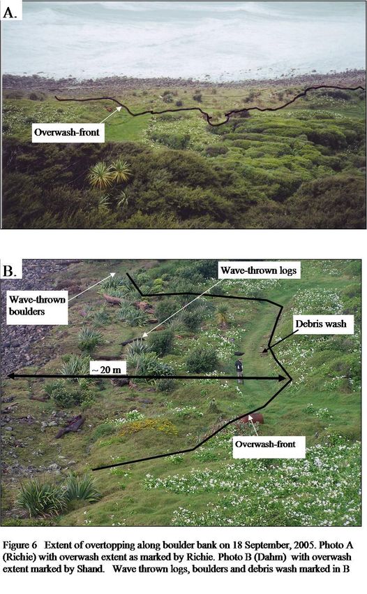
2

Executive Summary
In March 2006, Coastal Systems (NZ) Ltd were commissioned by Mr J Hemi to carry out
a thorough flood hazard assessment (from the sea) for his property at 108C Whanga
Road, Whale Bay, Raglan. The assessment was to include a review of the methodology
previously used to assess the predicted flood hazard elevation (as presented to the
Waikato District Council resource consent hearing in December 2005), acquire the
necessary and available data to accurately determine the flood hazard level for a 100 yr
return period event (this being the best practice value used in flood hazard assessment in
New Zealand), and accurately determine return periods for the storms in April, 1999 and
September, 2005 which caused some flooding at the margins of the property, and which
would be used to verify the predicted flood hazard level.

Review of the previous assessment identified significant error with mean sea level
(MSL), and also in the determination of the design elevations for the proposed dwelling.
These errors amounted to 1.3 m. The corrected MSL is 93.5 m relative to local datum.

The flood assessment was based on sea-level, barometric pressure and wind data obtained
from the New Zealand National Institute of Water and Atmospheric Research (NIWA),
deepwater wave and wind data obtained from the American National Oceanographic and
Atmospheric Administration’s (NOAA) global models, plus site-specific wave and run-
up data collected by Hamilton surveyors Skyworks Waikato Ltd. In addition, detailed
contour mapping was carried out by Skyworks. Data analysis was carried out by NIWA,
Coastal Systems (NZ) Ltd and Tonkin and Taylor Ltd. During the investigations,
discussions were held with Mr Jim Dahm, the Waikato District Council’s coastal
consultant, to ensure acceptable methodologies and assumptions were being used. It is
also noted that considerable effort went into assessing the effect of waves on flooding
because of the unique site characteristics – low relief and exposure to high wave energy.
For this reason, Tonkin and Taylor Ltd were commissioned to provide a report on
boulder bank run-up and overtopping implications for the proposed house site.

Part A of this report deals with the predicted flood hazard level. Standard statistical
procedures were used to derive the hazard component values (storm-surge, tide, wave
effect, intra and inter-annual sea-level variation and sea-level rise associated with global
warming). Two combinations of waves and storm surge were used: monthly waves with
a 0.9 m storm surge, and yearly waves with a 0.5 m storm surge. These combinations,
when coupled with the other hazard components give return periods well in excess of 100
yrs and the resulting hazard levels are thus conservative. The resulting predicted
inundation levels at the Hemi building site are 3.93 and 4.07 m above MSL (97.43 and
97.57 m local datum). These values are 0.13 to 0.27 m higher than the value of 3.8 m
used earlier at the December 2005 resource consent hearing.

Part B of the report deals with assigning inundation return periods to the storm events of
17 April, 1999 and 18 September, 2005. As continuous records of sea-level and
associated wave conditions are generally not available in NZ, return periods have to be
derived by using the components’ return periods and applying appropriate methods of
3

combination which depend on the likelihood of joint occurrence. Such an approach was
used in this investigation.

The 1999 event was found to have an inundation level at Whale Bay of ~3.0 m above
MSL (96.5 m local datum) and a return period less than 100 yrs. By comparison, the
2005 event had an inundation level of 3.36 m above MSL (96.86 m local datum) and a
return period equal to or greater than 100 yrs. These values are consistent with the
predicted flood hazard levels given above if 100 yrs of sea-level rise (0.45 m) is
excluded. Those values then become 3.48 to 3.62 m above MSL (96.98 to 97.12 m local
datum) and, as noted above, the predicted flood levels have a return period of at least 100
yrs.

A comparison of the predicted inundation levels (3.93 to 4.07 m above MSL) with the
critical assessment level of 4.2 m used at the 2005 hearing, this being the level of the
basement floor, shows that flooding during a storm equivalent to the hazard design event
will fail to reach this level by 0.13 to 0.27 m. While this may appear to be a relatively
small margin of safety, it is significant that the predicted inundation hazard level return
periods are well in excess of 100 yrs. Further confidence is provided by the site being
0.84 m above the flood level associated with the 2005 storm, an event found to have a
return period of at least 100 yrs.
4

                           TABLE OF CONTENTS

COVER PAGE                                                1
EXECUTIVE SUMMARY                                         2
TABLE OF CONTENTS                                         4
LIST OF TABLES                                            5
LIST OF FIGURES                                           6
LIST OF APPENDICES                                        6

INTRODUCTION                                              7

PART A INUNDATION ASSESSMENT                              9
     A1 Definition of inundation level                    9

      A2 Inundation recurrence                            9

      A3 Storm surge                                      10
            A3.1 Sea-level data
            A3.2 NZ-wide storm record
            A3.3 Assessment values

      A4 Tide level                                       11

      A5 Lower frequency sea-level fluctuations           11

      A6 Sea-Level Rise                                   12

      A7 Wave effects                                     12
           A7.1 Assessment wave heights
           A7.2 Wave effects from the sea
           A7.3 Wave effects from the lagoon
`               A7.3.1 Theoretically-based run-up
                A7.3.2 Empirically determined run-up
                        (i) Water-level approach
                        (ii) Lagoon run-up measurements
               A7.3.3 Discussion on lagoon wave effects

      A8 Discussion                                       22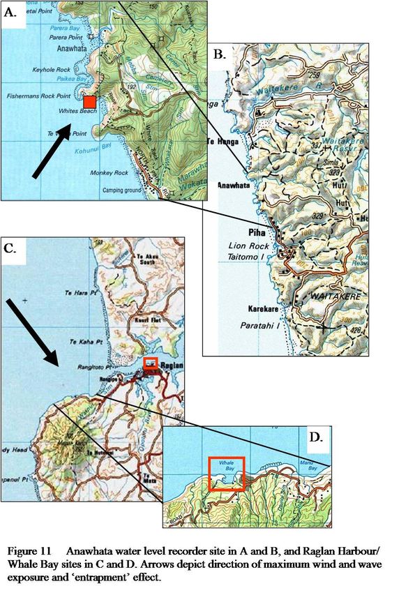
5

PART B RETURN PERIODS FOR TWO RECENT STORMS                                  23

     B1 Introduction                                                         23

     B2 Observed flood Impacts                                               23

            B2.1   Affidavit of Mr James Rickard
            B2.2   Debris, overwash and rock fracture
            B2.3   Water level comparisons
            B2.4   Anawhata sea-level data

     B3 Storm inundation parameters                                       34
           B3.1 April 1999 storm
           B3.2 September 2005 storm
           B3.3 Limitations of NOAA data for describing individual storms
           B3.4 Wave Growth Modelling
           B3.5 Wave height conclusions

     B4 Return period analysis                                                40
           B4.1 Component return periods
           B4.2 Computation methods for combining component return periods
                  (i)     Where sea-level data is available but simultaneous
                          wave data is not available
                  (ii)    Where sea-level data is not available but the other
                          Component data is available

DISCUSSION and CONCLUSIONS                                                   46

REFERENCES                                                                   47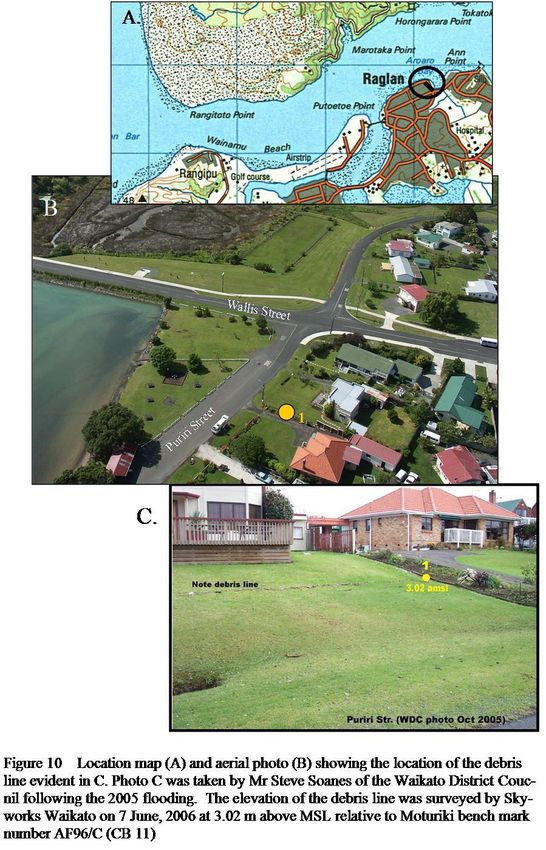
6
LIST OF TABLES
1. EVA of Anawhata storm-surge levels.
2. Calculated high tide levels and associated return periods for Whale Bay.
3. EVA output for deepwater waves and wind speed.
4. Shoaling and refraction transformations for westerly and northwesterly waves.
5. Theoretical and empirical lagoon run-up values normalized by wave height.
6. Summary of inundation values.
7. Flood levels for 1999 and 2005 storms at different locations.
8. Values and return periods of inundation forcing components: 1999 and 2005 storms.
9. Wave generation output based on the model Goda (2003).
10. Auckland Airport barometric pressure return periods.
11. Anawhata sea-level return periods.
12. Combinations of water level and wave marginal return periods for a 100 yr event.
13. Summary of inundation return periods using different methods.
14. Summary of elevations related to features and inundation.
LIST OF FIGURES
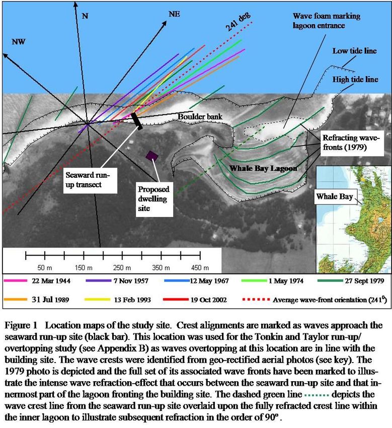
1. Wave crest alignments at boulder bank run-up transect.
2. Lagoon float measurements: site, equipment and deployment.
3. Water-level analysis output.
4. Photo of lagoon run-up maximum of 11 October, 2006.
5. Barometric pressure maps for September, 2005 and April, 1999 storms
6. Overtopping photos from September, 2005 storm.
7. Inundation extent from September, 2005 storm.
8. Contour plan of upper lagoon and dwelling site with inundation levels.
9. Block fracture by wave shock from the September, 2005 storm.
10. Flooding in Raglan Township from September, 2005 event.
11. Location of sea-level and flooding measurement sites at Anawhata and Whale
Bay/Raglan Township.
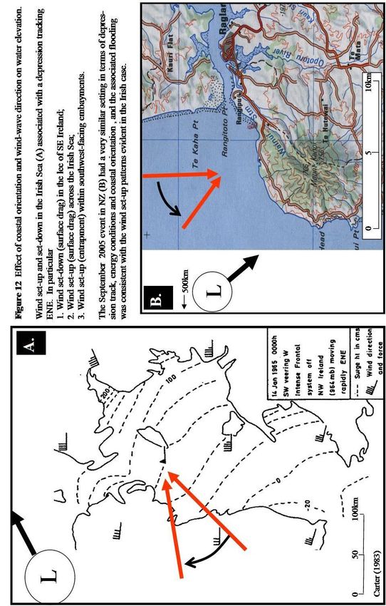
12. Effect of coastal orientation on water-level elevation: Irish Sea and Raglan.
13. Wind direction from Hamilton Airport for April, 1999 and September, 2005 storms.
14. NOAA wind and wave data for April, 1999 and September 2005 storms.
15. Barometric pressure from Hamilton Airport and from NOAA for 1999 and 2005
storms.
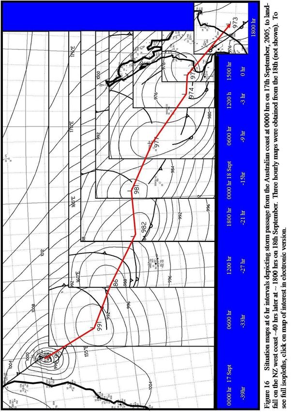
16. Situation maps for storm of September, 2005.
APPENDICES
A. Notes presented at the Hemi-WDC meeting, 8 June, 2006, by Roger Shand.
B Report on extreme run-up and overtopping of the boulder bank by Tonkin and Taylor.
C Affidavit of Mr James Rickard.
D McGowan Memo (Waikato District Council) on 1999 flood level in Raglan Township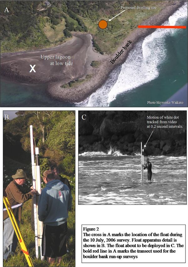
7

Introduction
An application by J Hemi for a Land Use Consent to construct a (second) dwelling at
108C Whanga Road (Fig 1) was heard by the Waikato District Council during 19-21
October, 2005 and 9 December, 2005. The hazard assessment presented by the
applicant’s coastal consultant, Dr Roger Shand of Coastal Systems (NZ) Ltd, at the
December hearing, was based on a standard inundation analysis using, where possible,
component values generally applicable to the NZ coast. Some site-specific professional
judgment for wave impacts was included. Verification of the predicted hazard level was
attempted by assigning return periods to storms that were known to have caused flooding
in the Whale Bay area in 1999 and 2005. However, the comprehensive data required to
accurately assess these storms was not obtainable within the available preparation time,
so they were qualitatively assessed using their physical characteristics, the extent and
nature of their environmental impacts and testimony by local residents. The council’s
coastal consultant (Mr Jim Dahm of Eco Nomos), and Dr Shand estimated the return
periods ranged between 10 yrs and 30 yrs. The 100 yr return period inundation level
(including a component for sea-level rise associated with global warming) was
determined to be 3.8 m above MSL, or 0.8 m above the floor of the basement, by Dr
Shand. Such occasional inundation was acceptable to the applicant as the dwelling had
been designed such that the floor level would be some 1.8 m above this predicted 100
flood level. While the council accepted the inundation value (3.8 m above MSL), the
application was declined, primarily on the basis that the council considered it
contravened NZCPS Policy 3.4.5 which states that “New subdivision, use and
development should be so located and designed that the need for hazard protection works
is avoided”.

J Hemi subsequently lodged an appeal with the Environment Court and in March, 2006
and instructed Coastal Systems to carry out a thorough flood hazard assessment. This
work was to include a review of the methodology previously used to assess the predicted
flood hazard elevation, acquire the necessary and available data to accurately determine
the flood level, and determine accurate return periods for the 2 storms which would be
used for verification.

The methods review found significant sources of error in the derivation of MSL, and also
in its application to determine the building’s design elevations. It is noted that time
constraints meant that both consultants (Coastal Systems and Economos) had to assume
materials provided to them prior to the 2005 hearings were accurate. These errors
subsequently resulted in the flood depths presented to the 2005 hearings being some 1.3
m too high! This unfortunate situation was explained to council staff at a progress
meeting held on 8 June, 2006. The means by which MSL was accurately determined are
explained in Appendix A, these materials being presented to Mr Dahm and council
officers at the 8 June meeting.

Mean sea level was fixed at 93.5 m relative to the local site datum; this compares with
the value of 94.4 m used earlier. The value of 93.5 m was selected on the basis of two
precise measurement exercises on the 23 March, 2006 and 21 April, 2006 which derived
8

values of 93.50 and 93.46 m. It is noted that a value of 93.6 m was tentatively used at the
8 June meeting and is presented in Appendix A, Table 3. However, this value was based
on the inclusion of two additional measurements (93.50 m and 93.53 m) derived during
exploratory field work on 22 February and 1 March, 2006 (as explained in Appendix A).
When these less reliable measurements are discarded, the value of 93.5 m becomes
appropriate and this was used as a basis for all subsequent measurement and analysis.

The corrections resulted in the 100 yr hazard level (3.8 m) now being 0.4 m below the
basement level compared with being 0.8 m above it as derived in the 2005 assessment.
However, it also meant that the 2005 storm flood level increased from 2.6 to ~3.4 m
relative to MSL. That storm flood level had previously been assigned a return period of
up to 30 yrs by the consultants based best professional judgment and the earlier MSL of
94.4 m. This new value now compares very closely with 3.35 m for the predicted 100 yr
hazard level (this being 3.8 m less 0.45 m for 100 yrs of sea-level rise, see Appendix A,
Table 3). This situation meant that either the assigned return period (up to 30 yrs) for the
September 2005 storm was too low, or else the predicted 100 yr flood level was too low.
This inconsistency was to be resolved during the forthcoming detailed assessment.

By December, 2006, the investigation was well advanced and discussions were held with
Mr Dahm at a meeting in Hamilton. The purpose of that meeting was to:

   •   Familiarize Mr Dahm with the research,
   •   Identify issues Mr Dahm considered needed further attention, and
   •   Reach agreement on a range of parameter/value options.

The final analysis and write-up of the full report was then undertaken.

The report contained herein consists of two parts: Part A derives the hazard inundation
level(s), while Part B assigns return periods to the 1999 and 2005 storms. Particular
attention has been paid to the acquisition and use of data collected by credible agencies
and subcontractors and to the collection and use of quality data from the site itself, to the
use of accepted statistical procedures to derive hazard components, their return periods,
and component return period combinations, and finally to ensuring caution when
selecting representative values. The results are summarized and conclusions drawn in the
final section of the report.
9

Part A. Inundation assessment

A1 Definition of inundation level

In New Zealand, it is considered best practice to use the following flood hazard
prediction formula:

Inundation level = storm surge + tide level + sea-level variation + sea-level rise + wave effects   (1)

Where the components consist of:
- storm surge = inverted barometric pressure + wind set-up;
- tide level measured relative to MSL;
- sea-level variation related to monthly to multi-decadal variation;
- sea-level rise (SLR) resulting from the effect of global warming;
- wave effects = wave run-up (swash plus wave set-up) plus overtopping considerations.

As noted earlier, general values are available for some components. However, for other
components it is desirable, and in some cases mandatory, to derive site-specific values
and this has been an major objective of the present exercise.

A2 Inundation recurrence

The agreed flood recurrence value is to be the 1% AEP (annual excedence probability),
i.e. 100 yr return period (RP). However, in the interests of caution, the derived flood level
exceeds this value.

Care has been taken to combine components using appropriate techniques based on
variable’ dependency-independency status and the probability of joint occurrence.
These concepts are considered in greater detail in section B3. However, it is noted here
that different return period combinations of two components can produce a 100 yr output.
For example a (relatively high) 10 yr tide occurring with a (relatively low) 0.03 yr (11
days) wave gives a 100 yr return period event, while a relatively low (0.03) tide
combined with a (relatively high) 10 yr wave also gives 100 yrs, as will numerous
intermediate combinations. The relative importance of water level and wave conditions
depend on the particular coastal response in question. Stability of engineering structures
is more dependent on wave height, while beach response tends to be a function of both
water level and waves. In the case of flooding by overtopping, it is water level that is
more important as wave effects will usually be ameliorated by depth limitation. It will be
shown in this report that water level is the predominant control at the Whale Bay site and
greater emphasis is made in the flood level computation process of relatively longer
water level return periods compared with those for waves for this reason.
10

A3 Storm surge

A3.1 Sea-level data
No sea-level data are available for the Raglan/Whale Bay area. The closest monitored
sites are at Anawhata (NIWA) and New Plymouth (Westgate), which are approximately
100 km and 150 km to the north and south respectively.
11

As the Anawhata sea-level record is the longer (7 yrs between 1998 to 2006), and as with
the Westgate record is also fragmented, NIWA were commissioned to undertake an
extreme value analysis (EVA) on the former. The raw sea-level measurements were first
corrected for missing or corrupt data and then each month of data was normalized by its
monthly average; this process was carried out to remove lower frequency variation in
MSL. Storm surge values were next obtained from the sea-level values by subtracting
corresponding inverted baromentric pressure values. NIWA’s extreme sea level analysis
software - EXTLEV was then used to identify the largest number of independent extreme
events per year (r-Largest Method), usually 5, and carry out a Gumbel fit. The resulting
extreme values are summarized in Table 1 and show the 100 yr return period (RP) storm
surge = 0.52 m. It is further noted that the difference between 10 yr and 100 yr RPs is 0.1
m.

Table 1 EVA of Anawhata storm-surge levels
 Return Period (yr)              5         10    20     50       100
Surge height* (m)            0.39        0.42  0.45   0.49      0.52
* relative to the mean level of the sea (MLOS)
Source: NIWA

While these results should only be considered broadly indicative of Whale Bay because
of the relatively short length of record and the contrast in coastal exposure between the
two sites (discussed later), some long-term extrapolation confidence is afforded for the
following reasons. The r-largest methodology used by NIWA fully utilizes the data but
traditional EVA only uses the highest value per year. In addition, confidence is increased
by the similarity of the barometric extreme values for 50 and 100 yr using the long-term
(41 yr) record from Auckland Airport and the more recent 7 yr record from Anawhata. In
particular, the 50 yr values are identical at 971.7 hPa, while the 100 yr are very close at
968.8 hPa c.f. 968.4 hPa. These results suggest that for this area the more severe events
have happened during the more recent period and the Anawhata data is more
representative of the longer-term than would otherwise be expected.

A3.2 NZ-wide storm-surge record
An extensive record of individual storms has been documented by Heath (1979), Hay
(1991) and Bell et al. (2000). Hay (1991) studied 153 storms and found the largest storm
surge to be 0.76 m, the second largest to be 0.49 m and 119 were less than 0.35 m. The
second largest recorded storm surge since 1890 was for Cyclone Giselle (1969) where
0.88 m was recorded in Tauranga Harbour (NIWA, 2000); an event which had a return
period of at least 450 yrs (de Lange, 1996). Based on extrapolation of available storm
data, storm surges in NZ have an upper limit of ~1m (Bell et al., 2000) and this consistent
for all NZ (Goring, 1995). However, the level corresponding to the 100 yr return period
would be considerably lower (NIWA, 2000).

A3.3 Assessment values
Based on the above results, it was agreed (Dahm-Shand meeting 5 December 2006) that
an upper and lower storm surge level would be assigned for the Whale Bay inundation
12

calculation. In particular, the lower value would be 0.5 m and the upper value 0.9 m.
Note that a value of 0.9 m was used for the December 2005 assessment. It is
acknowledged that the upper value will greatly exceed 100 yrs when combined with other
inundation components.

A4 Tide level

Tide levels and the associated EVA for Whale Bay were obtained from NIWA. These
data were obtained using their tidal model at 15 minute intervals over a 100 yr period.
The levels and return periods are given in Table 2. As tides and storm surge are
independent, their combined return period can be obtained by multiplying probabilities
(see section B3.2). Combining the mean high water spring (MHWS exceeded by 18.5%
of high tides) return period of 0.0075 yrs, with the 0.5 m storms surge’s return period of
20 to 50 yrs, and also the 0.9 m surge of > 100 yrs, gives return periods of 55 to 137 yrs
and >274 yrs respectively. As the combined return periods will greatly exceed 100 yrs in
all cases once wave effects are incorporated (see section A7.1 and section B3.2 Table
12), a lower tide level could be chosen. Indeed, even using the mean high water level’s
(MHW exceeded by 50% of high tides) RP of 1.17 m, the 100 yr threshold would be
exceeded once waves were incorporated. However, the more conservative tidal value of
1.4 m (exceeded by 25% of high tides) as used in the 2005 assessment will continue to be
used in the inundation computation. Note that this gives combined surge plus tide return
periods of 40 to 100 yrs for the 0.5 m surge and >200 yrs for the 0.9 m surge.

A5 Lower frequency sea-level fluctuations

Mean sea level may fluctuate over months to decades due to several longer-term factors
such as seasonal weather changes in temperature and windiness, ENSO-based climatic
oscillations and IPO shifts; the limited long-term open coast sea-level records suggest
inter-annual elevation changes of up to 0.2 m could occur (Bell et al., 2000). The storm-
surge values based on the individual storms (section A3.2) will have included such
variation. By contrast, the Anawhata storm-surge extreme values will be less influenced
as the input data had had at least a portion of this variation removed during preprocessing
as described earlier in section A3.1. This could certainly help explain the lower RP
values derived from the Anawhata sea-level data.

As the storm surge values selected for use in the inundation computation were higher
values based more on the individual storm data, and in recognition of the likelihood of
‘double dipping’ should a separate lower frequency sea-level variation component be
included in the calculation, it was agreed (Dahm-Shand meeting of 5 December, 2006)
not to include any such a component.
13

Table 2 Calculated high tide levels (above MSL) and return periods for Whale Bay

         Level (m)   Descriptor                           RP (days)   RP (yrs)
              1.17   Mean = 50% of all high tides                1      0.0027
              1.47   Spring = 18.6% all high tides            2.25      0.0075
              1.56   Pragmatical = 12% all high tides            4       0.011
              1.69   MHWPS = 4.8% all high tides                10       0.027
            1.775                                               30       0.082
              1.81                                              61       0.167
            1.826                                               92       0.252
            1.849                                              178       0.488
            1.863                                              267       0.732
            1.868                                              365             1
            1.884                                              730             2
            1.891                                            1095              3
            1.894                                            1460              4
            1.896                                            1825              5
            1.901                                          2737.5           7.5
            1.903                                            3650            10
            1.906                                            5475            15
            1.907                                            7300            20
            1.909                                          10950             30
            1.911                                          14600             40
            1.912    HAT Highest astronomical tide         18250             50
Source NIWA

A6 Sea-Level Rise

Hazard assessment requires a component be included to account for the projected rise in
sea-level over the coming 50 to 100 years. It is current best-practice to use the mid-range
projection for 100 yrs which has been given as 0.45 m by NIWA (2000), or 0.3 to 0.5 m
by MFE (2004). The value of 0.45 m, which was also used in the December 2005
assessment, will continue to be used in the present hazard calculation.

A7 Wave effects

Waves could affect the inundation levels at the building site either via overwash resulting
from run-up and overtopping of the seaward boulder bank, or via wave action within the
lagoon. Accounting for wave effects in the 2005 assessments was the main difficulty
encountered by consultants. It was therefore necessary to thoroughly investigate this
matter using site-specific data for calibration-verification. Boulder bank overtopping has
been addressed in a theory-empirical study by Tonkin and Taylor Ltd., whilst lagoon
effects have been addressed by a theory-empirical study carried out by Coastal Systems
(NZ) Ltd. However, before describing these studies and results, the deepwater wave
height to be used in the flood assessment will be determined.
14 A7.1 Assessment wave heights Joint probability analysis was undertaken to determine the combined return period of sea level with waves. This was carried out using the methods detailed in CIRIA (1996) which are detailed later in section B3.2(A) when considering the return period of the April 1999 and the September 2005 storms. The lower sea level estimate of 40 yrs in section A4 requires a wave height return period of 0.08 yrs to give a combined return period of 100 yrs. The remaining sea-level estimates of 100 to 200 yrs in section 4 would require no more than about average wave conditions. In keeping with a conservative approach it was decided to combine monthly return period waves with the 0.9 m storm surge, and yearly return period waves with the 0.5 m storm surge (Dahm-Shand meeting, 5 December, 2006). Wave parameters are generated at three hourly intervals by the National Oceanographic and Atmospheric Administration’s (NOAA) NewWaveWatch3 (NWW3) wave model, a third generation ocean wave propagation model which is the world standard. NWW3 uses wind fields to solve the spectral action density balance equation for wave number- direction spectra which can be applied to virtually any location on the planet. Significant wave heights, periods and directions for a site 3.5 km offshore and at 20 m depth were extracted for all 9 yrs of available wave data using the MetOcean Data Interface (MDI). These data were separated into 45 degree bins centred on NW, W, and SW. An EVA was performed using the MatLab suit which applied standard statistical procedures such as Weibull and Fisher-Tippet distributions to the 25560 sets of data. The best-fit solution was then selected to represent the return periods (see Table 3A). The EVA output in Table 3A shows similar results for southwesterly and westerly waves, with slightly higher waves from the southwest corresponding to return periods up to 1 yr, and higher waves from the west corresponding to the longer return periods. It is noted that a breakdown into smaller bins found that WSW waves actually had the highest values. Before deciding which wave direction to use when selecting the assessment values, several additional factors must be considered. Firstly, deepwater waves undergo shoaling and varying levels of refraction before reaching breakpoint at the site. These processes alter wave heights so their effects must be quantified. To determine the average refraction angles that apply to waves from the directional different bins during deepwater to breakpoint transformation, wave crests from available vertical geo-rectified aerial photographs (1944, 1957, 1967, 1974, 1979, 1989, 1993, 2002) were plotted in the vicinity of the boulder bank run-up transect (section A7.2). There should be a range of deepwater wave directions within a sample of this size. The average orientation of the 8 crest lines (Fig 1) was 241 deg (see dashed red line). There was a narrow range of angles (232 to 248 degrees) indicating all incident wave directions are able to refract to reach a similar final breaking orientation.
15

Table 3 EVA output for deepwater waves and wind speed

      A. Wave Analysis
      Return Period (yrs)            Northwest bin   West bin      Southwest bin
          fortnightly 0.042                   3.2          4.56              4.73
            monthly 0.083                    3.62          5.04              5.17
          3 monthly 0.25                     4.23          5.76              5.85
          6 monthly 0.5                       4.6          6.18              6.27
           9 monthly 0.75                     4.8          6.42              6.51
                                 1            4.9          6.65              6.48
                                 5           5.65          7.56              7.35
                                10           5.95          8.06              7.71
                                25           6.34           8.6              8.17
                                50           6.62          8.99              8.52
                               100           6.89          9.38              8.86
      B. Wind Analysis
      Return Period (yrs)            Northwest bin   West bin      Southwest bin
                                 1           19.09         19.61            20.06
                                 5           21.68         22.11            22.47
                                10           22.72         23.24            23.45
                                25           24.05         24.56            24.69
                                50           25.02         26.53             25.6
                               100           25.96         26.47            26.48
Data source: NOAA (see text)

These data indicate NW waves refract 16 deg to reach the run-up transect, W waves
refract 61 deg and SW waves refract 106 deg. As noted above, the largest waves in the W
bin (and hence those controlling the EVA output) are tending WSW, so they will undergo
in excess of 61 deg refraction.

From the wave-crests depicted in the 1979 photo underlying Fig 1, it can be seen how
the waves refract along the boulder bank and on into the lagoon until facing the building
site. At this point a wave has refracted about 90 deg beyond the orientation at the run-up
transect on the boulder bank. Note that the 1979 photo was the only one taken at high
tide and accompanied by large waves. Fortuitously, in this sample the crest line at the
run-up monitoring transect had an orientation of 241 deg which was the same as the
average value for all 8 samples.

Determining the wave height transformation from deep water to breakpoint during
refraction and shoaling was carried out using the DELFT Coastal and River Engineering
Software System (CRESS). Deep and shallow water wave characteristics are determined
using first and second order theory respectively, and shoaling and refraction determined
using standard equations. Monthly and annual return period wave height for the west
and northwest bins (Table 3) were transformed for the angles (Fi) noted above. The
average wave period (T) was determined for these waves and a slope-based coefficient
16
(γ) was also used as input. The modelling input and output values are summarised in
Table 4. Note that southwest bin waves were not been included as the deepwater wave
heights approximated westerly wave values and after the additional refraction, the
transformed heights were significantly lower.
The results in Table 4 show that the transformed westerly waves approximate the
transformed northwesterly wave heights. However, at noted above, the extreme westerly
waves actually have a more southerly direction and thus undergo greater refraction. For
example, another 10 degrees refraction (71 degrees) results in an additional 15 % height
loss. The results also show that the transformation affected the waves of each bin
differently with westerly waves reducing by approximately 22% at the breakpoint, while
northwesterly wave heights remained approximately the same. These results indicate that
for westerly waves the refractive loss dominated attenuation gain, while the opposite
effect occurred for NW waves. Overall, the results in Table 4 support the use of monthly
and yearly return period waves from the northwest for use in the inundation calculations.
Table 4 Shoaling and refraction transformations for westerly and northwesterly waves
Westerly waves Northwesterly waves
Monthly Yearly Monthly Yearly
Ho 5.25 6.65 4.11 4.9
T 11 11 10 10
γ 0.57 0.57 0.57 0.57
Fi 61 61 16 16
Hb 4.1 5.1 4.2 4.9
Input data sources: NOAA (waves), Raglan 1:200,000 Bathymetric Chart, Fig 1 (angles)
The use of NW waves is also appropriate as maximum storm surge (inverted barometric
pressure (iBP) and wind set-up) will accompany depressions originating in the north
Tasman Sea and then tracking SE to cross the west coast to the south of Raglan. This
allows the site to be affected by the maximum possible iBP and the maximum wind set-
up entrapment within the Mt Karioi embayment. This issue is discussed further in the
later Part B when describing the 1999 and 2005 storms.
A7.2 Wave effects from the sea
The likelihood of flooding at the proposed dwelling site via wave overtopping of the
boulder bank was the subject of an investigation by Tonkin and Taylor Ltd and their
report (Tonkin and Taylor, 2006) is attached as Appendix B. Briefly, this study consisted
of a run-up analysis followed by an overtopping analysis. The former was based on the
model used by Mr Dahm in his September, 2005 report to the Waikato District Council
(Eco Nomos, 2005). While the methodologies and numerical calculations were found to
be sound, several assumptions and parameter values were based on either incorrect
approximations or outdated information. Using site-specific run-up data collected under a17 range of wave conditions, it was possible to calibrate the model to fit the characteristics of the Whale Bay environment. Run-up elevations were produced for the range of water levels and wave heights likely to be experienced at the site. Results indicated that although overtopping would not be as severe as predicted in the Eco Nomos report, some overtopping is likely during certain water level and wave combinations. An assessment of overtopping discharges was then carried out. The applicability of the overtopping discharge model was verified by satisfactorily reproducing the 2005 storm overwash limit. Model output for the parameter values being used in the present assessment (sea-level = 95.85 to 96.25 [tide = 1.40, storm surge = 0.5 to 0.9 m, sea-level rise = 0.45 m, MSL = 93.5m], and wave height = 4.1 to 4.9 m, plus an order of magnitude safety factor), shows overwash would extend
18
The formula applies to irregular waves and has been confirmed under a range of incident
wave conditions (Guza and Thornton, 1981; Holman and Sallenger, 1985). It should be
noted that such extreme run-up formulations measure total run-up which includes wave
set-up and swash run-up.
While these formulae were developed for slopes >0.01, application of equation (1) to
lower slope situations is generally made on the grounds that it over-predicts run-up from
field data (Holman, 1986) by a factor of two. In addition, for the Whale Bay lagoon
situation, further application assurance is given by reduced wave energy reaching the
shore due to storm waves having already undergone breaking at the mouth of the lagoon
(see Fig 1) and reformation before travelling across the lagoon, refracting, and finally re-
breaking prior to run-up. Note that the lagoon entrance is only about 1 m below MSL, so
under extreme water levels (MSL + 2 to 2.5 m) waves higher than about 1.8 to 2.1 m are
depth limited. Considerable wave energy is lost during this initial breaking process with
field measurements showing reformed waves rarely contained more than 20-40% of their
incident value (Carter and Balsille, 1983). This argument assumes that the controlling
rocky morphological configuration of the spit and lagoon will remain the same during the
next 50 to 100 yrs. This assumption is reasonable based on no change being evident
when inspecting the superimposed aerial photos; in fact individual boulders and clusters
of boulders could be matched.
Using T = 10s, tan β = 0.012, Hmonthly = 4.1 m and and Hyearly = 4.9:
• Lo = 156 m, (equation 4);
• ﻉ0 = 0.074 for Hmonthly and 0.068 for Hyearly (equation 3), and
• R 2% = 1.20 m for Hmonthly and 1.35 m for Hyearly (equation 2), which results in
wave-normalized values of 0.292 and 0.275 respectively. These normalized run-
up values (coefficients) appear in Table 5.
Table 5 Theoretical and empirical lagoon run-up values normalized by wave height*
Run-up method Hmonthly = 4.1 m Hyearly = 4.9 m Hbsig
R2% (equation 2) 0.292 0.275
Water level (10.7.06) 0.28
Run-up (11.10.05) 0.258
*Normalization for equation 2 output was with respect to NW extreme wave height values.
Normalization for empirically determined values was Hbsig (which was measured concurrently at
the boulder bank run-up transect, see Tonkin and Taylor (2006), Table 2), transformed to Ho for the NW sector.
A7.3.2 Empirically determined run-up
Lagoon run-up under higher wave and tide conditions was carried out using water level
data and run-up data.19 (i) Water-level approach This approach was based on the analysis of a water-level record that was obtained using a float arrangement (Fig 2) that was tracked by video camera. The apparatus was located within the lagoon in a region observed to have maximum surface fluctuation (Fig 2). The survey was carried out over the 8.40 am high tide on 10 July, 2006 when a run-up survey on the boulder bank was also underway, Hb data were thus available for use in the analysis. Environmental conditions were: tide = 1.05 m; storm surge (average of Anawhata and Westgate) = -0.1 m; Hbsig = 4.8 m; T = 16.5 s. Using the CRESS wave transformation model, equivalent Ho from the NW sector = 3.95 m. The water-level data were abstracted using an image processing algorithm written by Professor Donald Bailey of the Institute of Information Sciences and Technology at Massey University. A sample of the record is depicted in Fig 3A while the full 40 minute record is represented by the histogram in Fig 3B. Note that the lower frequency wave motions evident in Fig 3A are at ~3 min intervals. This value was similar to the wave group periodicity observed during the seaward run-up survey and was expected given the low slope in the lagoon. The maximum reformed wave height is estimated at 1.1 m. Note that 0.1 m has been added to the signal to compensate for truncation of the lower values as explained in the caption for Fig 3. While exact conversion of the maximum wave height to run-up is not possible, it is noted that on sandy beaches run-up is usually much less than the height of waves seaward of the breakpoint, this reduction being due primarily to friction and turbulence. However, where lower frequencies predominate and topography influences wave behaviour, maximum run-up could conceivably equal wave height. In this situation the normalized run-up value would be 1.1/3.95 = 0.280 m and this result has been included in Table 5. (ii) Lagoon run-up measurements Run-up elevations were obtained from a video record taken during the 13.15 hr high tide of 11 October, 2006 when the final run-up survey was being conducted on the boulder bank. Environmental conditions were as follows: tide = 1.44 m, storm surge (average of Anawhata and Westgate) = 0.04, Hb sig = 4.5 m and T = 15 s. Using the CRESS wave transformation model, equivalent Ho from the NW sector = 3.8 m. Elevations corresponding to the three highest run-ups were 95.96 m 95.90 and 95.86 m. A frame depicting the highest run-up appears as Fig 4. Subtracting tide, storm surge and mean sea level from the highest elevation (95.96 m) gives a run-up value of 0.98m. Normalizing this value with respect to NW sector deepwater wave height gives 0.98/3.8 = 0.258. This value has been added to Table 5.
20
21
22

A7.3.3 Discussion on lagoon wave effect

The normalized theoretical and empirical run-up values (coefficients) in Table 5 are
remarkably close, ranging between 0.258 and 0.292, and give confidence to the
methodologies. It is also helpful that the most reliable estimate, the actual run-up
measurement made under higher wave and tide conditions (0.258), happens to be the
lowest value. A representative value for the lagoon wave effect coefficient of 0.323 was
selected for use in the inundation calculation; as this value provides a 25% safety margin
over the most reliable value of 0.258.
23

A8 Discussion of Part A (inundation assessment)

Component values derived in the preceding sections have been summarized in Table 6.
The predicted inundation levels at the Hemi building site, using established and/or agreed
to criteria, range between 3.93 and 4.07 m above MSL (97.43 and 97.57 m above local
datum). These values are 0.13 to 0.27 m higher than the value (3.8 m) proposed at the
December 2005 hearing,

Table 6 Summary of inundation values
     WAVES:                         Hmonthly=4.1 m   Hyearly = 4.9 m
     Storm surge                             0.9               0.5
     Tide                                    1.4               1.4
     Sea level variation                       0                  0
     Wave effect_sea                           0                  0
     Waves effect_lagoon: 0.323*H           1.32              1.58
     SLR                                    0.45              0.45
     Totals (MSL datum)                     4.07              3.93

     MSL                                   93.5             93.5
     Totals (local datum)                 97.57            97.43
24 Part B. Return Periods for two recent storms events B1 Introduction Two particularly energetic storms recently caused flooding in the vicinity of the proposed dwelling, so assigning return periods to these events provides a means of validating the design inundation levels. The storms are particularly interesting as they were caused by contrasting weather systems. The first on the 17 April, 1999, was driven by a depression which crossed the lower South Island, while the second on the 18 September, 2005, had a more northward origin and crossed the North Island near New Plymouth (see Fig 5). The characteristics of the two events will now be described in some detail; firstly based on observed damage and then based on storm parameter values derived from meteorological and oceanographic data. The return periods of these parameter values will then be derived using extreme value analysis and combined to provide event inundation return periods. B2 Observed flood Impacts B2.1 Affidavit of Mr James (Tex) Edwin Lancelot Rickard Mr Rickard moved to Raglan 1945 to work at the Post Office. He has lived and farmed about Te Whaanga and developed a particular awareness of storms and coastal processes
25
through decades of metrological reporting and organizing coastal erosion conservation
programmes. Mr Rickard’s observational credibility must be respected. His full affidavit
attached as Appendix C. Of particular relevance are paragraphs 5 and 6 (reproduced
below) which relate to flooding in general and to the September 2005 storm in particular.
5. I understand that Mr Hemi applied for a resource consent to build a home on
his ancestral land but his application was declined by the Waikati District
Council and is now subject to appeal. The council seem to think the sea will flood
this land. I have never seen this area flood or heard of it flooding in all my time in
Raglan.
6. I used to spend a lot of time at Te Whaanga planting native trees, fencing,
gardening, cleaning up around my wife's bach (which my youngest son has inherited)
and generally relaxing with our extended family. From the bach window I can see the
remains of last year's September storm. Logs and rocks are still lying on the edge of
the land, beside the pohutukawa tree. The land didn't flood, but the sea overtopped
the edges in places
B2.2 Debris, overwash and rock fracture
The extent of the September 2005 event has been well recorded in photos and surveys.
The site was visited by Mr Dahm on 19 September 2005 while the storm was still
subsiding and a comprehensive set of photographs taken and reported (Eco Nomos,
2005). The site was also visited by the author on 12 October with follow up visits in
June, 2006 and October, 2006. During these visits photographs and measurements were
taken. Photos were also taken by Professor Richie.
Figure 6 contains 2 photos depicting the overwash extent along the boulder bank with
wave-thrown boulders, logs and general debris having been marked.
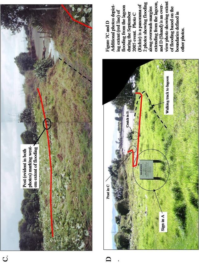
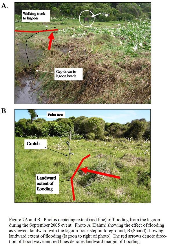
Figure 7 contains several photos detailing the extent of flooding from the lagoon.
Figure 8 locates the maximum flood elevation (96.86 m) as determined by Skyworks
Waikato based on the debris-front and vegetation damage. The flooding extended some
16 m landward of the lagoon embankment and reached some 25 m from the proposed
dwelling site. As noted in the Introductory section, MSL at Whale Bay has been fixed at
93.5 m so the flood elevation reached 3.36 m above MSL.
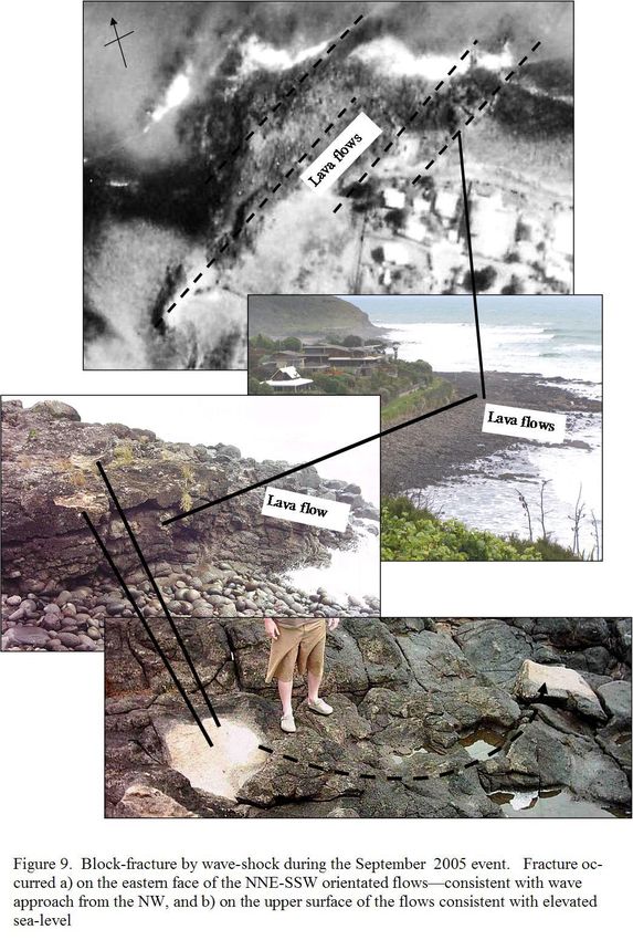
Figure 9 shows the location and nature of rock fracture via the process of wave shock on
the lava bluffs and promontories bounding the eastern side of the lagoon entrance. Such
fracturing only occurred on the NE side of the lava flows, this being consistent with the
NW waves which characterized this storm. They also occurred on top of the flows as
would be expected during elevated water levels when the waves could reach these areas.
The light coloured scars where lava blocks were removed were still clearly discernable
over a year after the event. The author has not observed such fracturing before, indicating
the rarity of such an event.26
27
28
29

By comparison, there is much less evidence as to the impact of the April 1999 event at
the site. Some photos were presented at the October 2005 hearing by Professor Richie.
One showed wave action at the lagoon step and this has allowed a tentative elevation to
be reconstructed and marked on the contour map (Fig 8) at 96.5 m (3.0 m above MSL).
This level, together with the 2005 level of 96.86 m (3/36 m above MSL) are included in
Table 7 which summarizes the different flood levels at different locations.

Table 7 Flood levels (m)* for 1999 and 2005 storms at different locations
       Event     Whale Bay       Raglan Harbour     Anawhata

          1999   ~3.00                       2.85              2.16
          2005    3.36                       3.02              1.76
      * Whale Bay and Raglan Harbour levels based on Moturiki datum.
       Note local datum at Whale Bay = 93.5 m
       Anawhata datum is mean level of the sea (MLOS) over the recording period.

Another of the Richie photos showed a wave-thrown log. This evidence, together with
comment by other local residents that relatively little environmental damage
accompanied that event, indicates the 1999 storm had less local impact than the 2005
event.
30
31

B2.3 Water level comparisons

A reliable water level from Raglan Harbour (3.02 m above MSL) was obtained by
leveling a well defined debris line from a photograph taken by Waikato District Council
staff following the September, 2005 flood (see Fig 10). The site is in the vicinity of
Aroaro Bay on the northern side of the township and was thus well sheltered from the
direct effect of oceanic incident waves. This 2005 level compares with 2.85 m for the
1999 event in the same location as measured by Waikato District Council staff (see
APPENDIX D). These flood levels are included in Table 7. The Raglan results
qualitatively support the observation at Whale Bay that the 2005 flood level exceeded the
1999 level.

B2.4 Anawhata sea-level data

The NIWA sea-level recorder at Anawhata just north of Piha on the Auckland west coast
also provided comparative data for the 1999 and 2005 events and this result has also been
included in Table 7. The values are significantly lower than the corresponding Whale Bay
and Raglan Harbour values and this is to be expected as wave effects have been filtered
from the Anawhata output, there is no freshwater contamination, and a different elevation
datum applies. However, what is particularly noteworthy is the relative elevation
reversal with the 1999 value being substantially greater than the 2005 level. An
explanation of this difference is particularly important because it would offer insight into
why such significant flooding occurred in September, 2005 at Whale Bay/Raglan while
such flooding was absent on much of the west coast.

The location of the Anawhata recorder and the Raglan sites are depicted in Fig 11A-D.
The two areas have contrasting geographic orientation with Anawhata (A and B) being
exposed to the southwest and Raglan (C and D) to the northwest. Anawhata could be
expected to undergo wind and wave set-up during southwest conditions, while probably
undergoing wind set-down under northwest conditions. These effects would be reversed
at Raglan, and magnified due to the size of the Mt Karioi headland. The former process
(wind set-up) is enhanced by topographic ‘entrapment’ of surface waters, while the latter
(set-down) occurs when surface water being blown seaward faster than it can be replaced
by upwelling. Such processes are well documented and Fig 12 is included as an example.
It is noted that at Raglan, winds from WNW (292.5) appear to be at the southern limit of
entrapment.

Different hydrodynamic conditions will therefore have differing process-responses at the
two sites. As will be seen in the following section, contrasting conditions occurred
during the 1999 and 2005 events with northwest domination during the latter resulted in
enhanced elevations at Raglan, while southwest domination during the former resulted in
relatively higher levels at Anawhata and less flooding at Raglan.
32
33
34
35

B3 Storm inundation parameters

B3.1 April 1999 storm
The 1999 event occurred on the 17th April during the 10.18 hr (am) high tide; this was an
exceptionally high spring tide exceeded only 6 times per year. The magnitude of the
inundation components are summarized in Table 8A. Note that associated return periods
are also listed and these values, together with their derivation, will be considered further
in section B4. The wind direction record from Hamilton Airport (Fig 13) shows winds
were essentially south of the entrapment threshold for 5 hours preceding the high tide and
remained so thereafter. NOAA Global Forecast System (GFS) wind data for a site 3.5
km offshore (Fig 14 left column) show maximum speeds occurred just prior to the high
tide. These data have been used in preference to the Hamilton Airport wind speed record
because of significant topographic interference between the ocean and airport. In the lee
of the Raglan headland the strong WSW wind may well have resulted in sea surface set-
down. NOAA NWW3 wave data (Fig 14 left column) show waves during this time were
rapidly increasing in size and period, and arriving from the WSW. Barometric pressures
from Hamilton Airport and NOAA are shown in Fig 15A. The NOAA predicted
minimum value is slightly lower and earlier than the observed value at Hamilton Airport.
The airport data is used in Table 8 with a 1 hr offset to account for the temporal lag
between the open coast and airport.

Table 8 Magnitudes and return periods of inundation forcing components
  for the storms of April, 1999 and September, 2005.
     A. 17 April, 1999. 1018 hr high tide
     Component            Magnitude                      Return Period (yrs)
     Tide (m)                                    1.81    0.16 (58 days = 6x /yr)

     iBP (m) (990.5)                             0.24    0.023 (8.5 days = 43x /yr)

     Wind (m/s)                                  19.1    0.49 (179 days = 2x /yr)
                                      WSW   (250o)
     Waves (m)
36 B3.2 September 2005 storm The 2005 event occurred on the 18th September during the 21.48 hr spring high tide. Note that significant overtopping of the port breakwaters occurred at Port Taranaki on this tide and significant erosion happened at Muriwai Beach; both locations having northwesterly exposure similar to Raglan. This high tide level (Table 8B) was only slightly less than the 1999 level (1.78 c.f. 1.81 m). The wind direction record from Hamilton Airport (Fig 13) shows winds were north of the entrapment threshold for the whole day (from 60 deg around through 360 deg and on down to the threshold of 293 deg) leading up to the evening tide and only crossed the threshold an hour or so before the tidal maximum. It is therefore likely that wind set-up would still have been contributing to the storm surge during the high tide. NOAA Global Forecast System (GFS) wind data show maximum speeds were occurring during the high tide just prior to the high tide (Fig 14 right column). The NOAA NWW3 wave data (Fig 14 right column) show waves during this time were from the NW and building both in size and period. While deepwater height magnitudes were less than the 1999 levels (4.11 m c.f. 6.63 m), the more northerly approach (305 deg c.f. 245 deg) ensured the 2005 waves underwent less subsequent refractive energy loss. While minimum pressure (maximum inverted barometer) occurred four hours prior to the high tide and the pressure had risen some 7.5 hPa, the level was still ~10 hPa lower than during the 1999 high tide (see Fig 15). Of particular significance in Fig 15B is the temporal variation between the NOAA predicted data and the observed Hamilton Airport data (used in Table 8). This situation will now be discussed further.
37
38

B3.3 Limitations of NOAA data for describing individual storms

While NOAA produces forecast data which is subject to continual update, it is
nonetheless based on wind-field prediction, and weather system behaviour in the final
hours may differ from modelling expectation. Indeed, this appears to have happened
during the 2005 event in particular, as indicated by comparing the observed (Hamilton
Airport) and predicted (NOAA) barometric pressure graphs in Fig 15B. While observed
pressures were ~ 5 hPa higher than predicted, thus reducing the potential storm surge, the
depression itself appears to have also moved slower than expected. The difference
between the 1999 predicted and observed data (Fig 15A) is much less and probably
within variation associated with offset (airport to coast) and sampling resolution. The 4-5
39

hours difference between the 2005 data sets, however, could have significant implications
for wind and wave effects. Firstly, the delay would have allowed the development of
larger waves, and possibly also of stronger winds, than those predicted by NOAA, and
secondly, the earlier wind and wave approach direction (NW) would have persisted
longer than predicted. The values in Figure 14 right column and Table 8B may therefore
underestimate the actual values. The effect such storm delay would have on the wave
data will be assessed using the wave growth model of Goda (2003). However, before this
is carried out, another weakness of the NOAA model as pertains to describing individual
storms, c.f. describing wave climate, will be described, as this can also be assessed by the
Goda wave growth model.

Prior to 2006, NOAA NWW3 wave data was ‘broadly directional’ in that once a new
wave train entered a model grid point, it was combined with the existing train to give an
‘average’ height, period and direction. NOAA now produce a spectrum of directional
output. While this earlier methodology is not expected to have much effect on wave
climate output, it does have implications when wave trains are changing - as occurred
during the 2005 event. In particular, the magnitude or direction of waves from the
dominant train could be undervalued by the combination process. This situation not only
has implications for the wave height, but it may change the period and directional bin –
the latter resulting in the assignment of a different return period. In the 2005 situation the
earlier and higher impact northwest waves could be contaminated by subsequent west to
southwest waves and hence be assigned a lesser return period.

B3.4 Wave Growth Modelling
Input parameters for the Goda wave growth model consisted of wind speed, fetch (F) and
duration. Parameter values were derived from 3 to 6 hourly situation maps obtained
from NIWA. Overlaying the situation maps (6 hourly samples only) showed isobars
directed toward the North Island from when the depression appeared off the Australian
coast (Queensland-NSW border) on the 0000hr map of 17th September. However, the
directional spread increased until the map of 1800 hrs (17th Sept) when isobars became
more uniformly directed at the mid North Island west coast, and speeds rose to be in
excess of 20 m/s thereafter. A value of 20 m/s was selected as the input value. Fetch on
individual maps ranged between ~300 and 600 km and the ‘system-translation fetch’
essentially extended from the initial map. All output was found to be fetch unlimited.
Storm durations from 9 hrs to 50 hrs were used. Resulting H0sig and T0sig output,
together with the differences between sequential H0sig values, are shown in Table 9.

Table 9 Wave generation output based on the model Goda (2003)
Wind
duration
(hrs)            9        12         15        18         21        24         30        40          50
H0sig
(m)           4.14      4.76       5.27        5.7      6.08      6.41       6.96       7.67         8.2
Hdiff           -       0.62       0.51      0.43       0.37      0.33       0.55       0.71        0.53
T0sig          7.4       8.1       8.66      9.13       9.54      9.89      10.48     11.25        11.83
40

Firstly, it is noted that the longest wave periods in Table 9 correspond to NOAA’s 11.7s
value appearing in Table 8B. However, this situation would require full wind contribution
from the time the depression first appeared and would have generated waves heights of
~8 m. It seems more plausible that wind contribution occurred during the final 24 hours
(mid -21 hr and -27 hr maps, see Fig 16) as indicated by the isobars (~wind direction) on
the situation map of 1800 hr (-21 hrs) becoming more directed toward the mid North
Island and remaining so thereafter. The longer period NOAA waves would then be an
artifact of the spectral combination method described earlier. Indeed, the hump on the
wave period time series (circled in Fig 14) suggests super-positioning of 2 wave trains.
In this situation of 24 hrs of wave growth, the wave height of 6.41 m is still well in
excess of NOAA’s value of 4.11 m (Table 8B). Once again, this is demonstrably an
artifact of the spectral combination method!

Secondly, if the storm delay of 3-6 hours indicated in Fig 15B is taken into account, then
NOAA would have been modelling based on 18 to 21 hours instead of 24 hours. The
delay would have resulted in an underestimate of wave growth by ~ 0.3 to 0.7 m (say 0.5
m). NOAA’s value of 4.11 m should thus be increased to 4.41 to 4.81 m.

B3.5 Wave height conclusions
The results of the wave analysis show that waves accompanying the 2148 hr tide on 18th
September, 2005 would have been in the range 4.5 to 6.5 m rather than the 4.11 m
predicted by NOAA.

In addition, when the increase in wave height for the 2005 event is coupled with the
greater refractive energy loss experienced by the 1999 event’s 6.63 m deepwater waves
from the southwest, the waves affecting shoreline run-up on the 18 September, 2005
would very likely have been larger.

B4 Return period analysis

Determining the return period for a flood-inducing storm often requires knowledge of the
probability of occurrence of individual component variables. Component return periods
are considered in section B4.1, while combining the component return periods is dealt
with in section B4.2.

B4.1 Component return periods
Return periods were calculated using extreme value analysis (EVA) applied to the
maximum value per year from the available data-set, or in some cases the several highest
independent values per year were used.

As noted already, this study has used wind and deepwater wave data obtained from
NOAA. In particular, all 9 years of available data (1997 to 2006) were obtained for a
location 3.5 km offshore. Several different distribution shapes were used in the analysis
and the best fit selected to derive the extreme values and associated return periods. While
a longer sampling period would of course be preferable, several years are considered
You can also read