Large-volume air sample system for measuring 34S/32S isotope ratio of carbonyl sulfide - Atmos. Meas. Tech
←
→
Page content transcription
If your browser does not render page correctly, please read the page content below
Atmos. Meas. Tech., 12, 1141–1154, 2019
https://doi.org/10.5194/amt-12-1141-2019
© Author(s) 2019. This work is distributed under
the Creative Commons Attribution 4.0 License.

Large-volume air sample system for measuring 34S/32S isotope
ratio of carbonyl sulfide
Kazuki Kamezaki1 , Shohei Hattori1 , Enno Bahlmann2 , and Naohiro Yoshida1,3
1 Department  of Chemical Science and Engineering, School of Materials and Chemical Technology,
Tokyo Institute of Technology, G1-17, 4259 Nagatsuta-cho, Midori-ku, Yokohama 226-8502, Japan
2 Leibniz Centre for Tropical Marine Research, Fahrenheitstraße 6, 28359 Bremen, Germany
3 Earth-Life Science Institute, Tokyo Institute of Technology, 2-12-1-IE-1 Ookayama, Meguro-ku, Tokyo 152-8550, Japan

Correspondence: Shohei Hattori (hattori.s.ab@m.titech.ac.jp)

Received: 25 September 2018 – Discussion started: 15 October 2018
Revised: 8 February 2019 – Accepted: 11 February 2019 – Published: 22 February 2019

Abstract. Knowledge related to sulfur isotope ratios of car-      in cylinders and collection processes for that sample. The dif-
bonyl sulfide (OCS or COS), the most abundant atmospheric         ference of atmospheric δ 34 S(OCS) values between 10.5 ‰ in
sulfur species, remains scarce. An earlier method developed       Japan (this study) and ∼ 13 ‰ recently reported in Israel or
for sulfur isotopic analysis for OCS using S+ fragmenta-          the Canary Islands indicates that spatial and temporal varia-
tion by an isotope ratio mass spectrometer is inapplicable        tion of δ 34 S(OCS) values is expected due to a link between
for ambient air samples because of the large samples re-          anthropogenic activities and OCS cycles. The system pre-
quired (approx. 500 L of 500 pmol mol−1 OCS). To over-            sented herein is useful for application of δ 34 S(OCS) for in-
come this difficulty, herein we present a new sampling sys-       vestigation of OCS sources and sinks in the troposphere to
tem for collecting approximately 10 nmol of OCS from ambi-        elucidate its cycle.
ent air coupled with a purification system. Salient system fea-
tures are (i) accommodation of samples up to 500 L (approx.
10 nmol) of air at 5 L min−1 ; (ii) portability of adsorption
tubes (1/4 in. (0.64 cm) outer diameter, 17.5 cm length, ap-      1   Introduction
proximately 1.4 cm3 volume) for preserving the OCS amount
and δ 34 S(OCS) values at −80 ◦ C for up to 90 days and           Carbonyl sulfide (OCS) is the most abundant sulfur-
14 days; and (iii) purification OCS from other compounds          containing gas in ambient air with atmospheric concentra-
such as CO2 . We tested the OCS collection efficiency of          tions of approximately 500 pmol mol−1 in the troposphere
the systems and sulfur isotopic fractionation during sam-         (Chin and Davis, 1995; Montzka et al., 2007). In fact, OCS
pling. Results show precision (1σ ) of δ 34 S(OCS) values as      can be transported to the stratosphere because the average
0.4 ‰ for overall procedures during measurements for at-          residence time of OCS is longer than 2 years (Brühl et al.,
mospheric samples. Additionally, this report presents diurnal     2012). In the stratosphere, it is converted to stratospheric
variation of δ 34 S(OCS) values collected from ambient air at     sulfate aerosols (SSAs) through atmospheric sink reactions
the Suzukakedai campus of the Tokyo Institute of Technol-         (Crutzen, 1976). Therefore, OCS must be regarded as an im-
ogy located in Yokohama, Japan. The observed OCS con-             portant sulfur source for SSAs, playing an important role in
centrations and δ 34 S(OCS) values were, respectively, 447–       the Earth’s radiation budget and in ozone depletion. More-
520 pmol mol−1 and from 10.4 ‰ to 10.7 ‰ with a lack of           over, because leaves consume OCS whenever assimilating
diurnal variation. The observed δ 34 S(OCS) values in ambi-       CO2 but do not emit OCS to the atmosphere by respiration
ent air differed greatly from previously reported values of       (Sandoval-Soto et al., 2005), OCS can be a tracer of gross pri-
δ 34 S(OCS) = (4.9 ± 0.3) ‰ for compressed air collected at       mary production (GPP) on land (Campbell et al., 2008). For
Kawasaki, Japan, presumably because of degradation of OCS         those reasons, elucidating the OCS dynamics in the atmo-
                                                                  sphere is important to elucidate the carbon cycle. Neverthe-

Published by Copernicus Publications on behalf of the European Geosciences Union.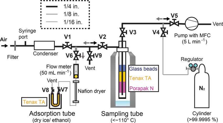
1142                                                 K. Kamezaki et al.: Measuring 34 S/32 S isotope ratio of carbonyl sulfide

less, tropospheric OCS sources and sinks entail great uncer-       centrations at pmol mol−1 levels in ambient air (Bahlmann
tainty (Watts, 2000; Kremser et al., 2015) because of miss-        et al., 2011). Subsequently, we combined this sampling sys-
ing sources in the atmospheric budget of 230–800 Gg a−1 S          tem and newly developed an online OCS purification sys-
equivalents as revealed by top-down modelling (Berry et al.,       tem for separation from impurities such as CO2 , which is
2013; Glatthor et al., 2015; Kuai et al., 2014).                   106 times more abundant in air than OCS. For the current
   Isotope analysis is a useful tool to trace sources and trans-   study, we describe the systems and its applications to atmo-
formations of trace gases (Johnson et al., 2002; Brenninkmei-      spheric observation. We provide first results for diurnal vari-
jer, 2003). To quantify OCS sources and sinks in natural en-       ations of δ 34 S(OCS) in ambient air from samples collected at
vironments using isotope analysis, determination of isotopic       the Suzukakedai campus of the Tokyo Institute of Technol-
fractionation for reactions and ambient measurements is re-        ogy located in Yokohama, Japan.
quired. To date, isotopic fractionations occurring in the reac-
tions of OCS have been determined for almost all OCS sink
reactions in the stratosphere: OCS photolysis (Hattori et al.,     2     Materials and methods
2011; Lin et al., 2011; Schmidt et al., 2013) as well as re-
actions with OH (Schmidt et al., 2012) and O(3 P) (Hattori         2.1    Samples
et al., 2012). Furthermore, the sulfur isotopic fractionation
during soil bacterial degradation and enzymatic degradation        An overview of the synthetic samples used for method eval-
was ascertained based on laboratory experiments (Kamezaki          uation in this study is given in Table 1. Commercial sam-
et al., 2016; Ogawa et al., 2017). Based on the analysis of        ples containing 10.5 % OCS balanced with high-purity He
commercially available compressed air, our group suggested         as sample A (99.99995 % purity; Japan Fine Products Co.
a δ 34 S value of (4.9 ± 0.3) ‰ for tropospheric OCS (Hattori      Ltd., Kawasaki, Japan) and 5.9 µmol mol−1 OCS balanced
et al., 2015). However, very recently, Angert et al. (2019)        with high-purity He as sample B (99.99995 % purity; Japan
reported a markedly different δ 34 S value of (13.1 ± 0.7) ‰       Fine Products Co. Ltd.) were used (Table 1). Furthermore,
for tropospheric OCS using a gas chromatograph (GC) –              we synthesized OCS from three kinds of sulfur powders, des-
multi-collector inductively coupled plasma mass spectrom-          ignated as sample C produced from sulfur power (99.99 %
eter (MC–ICP-MS). For the measurement of sulfur isotope            purity; Fujifilm Wako Pure Chemical Corp., Japan), sam-
ratios (δ 33 S, δ 34 S, and 133 S values) of OCS in our labo-      ple D produced from sulfur powder (99.98 % purity; Sigma-
ratory, an online method measuring on a GC–isotope ratio           Aldrich Corp. LLC, Missouri, USA), and sample E (a mix-
(IR)–MS using S+ fragmentation ions had been developed             ture of sulfur powders used for samples C and D) with a reac-
(Hattori et al., 2015). This method supports simple analysis       tion with CO (99.99 % purity; Japan Fine Products Co. Ltd.,
of sulfur isotopic compositions of OCS over 8 nmol. How-           Kawasaki, Japan) in a manner similar to that described by
ever, application of this method for atmospheric samples has       Ferm (1957) and Hattori et al. (2015) (Table 1). The OCS
yet to be carried out using this GC–IR-MS method because           concentrations for samples A and B were determined against
of the large sample amounts that are necessary (i.e. 500 L         the in-house synthesized OCS (i.e. 100 %) diluted to 10 %
of 500 pmol mol−1 OCS). Therefore, we aimed to develop             using high-purity He (99.99995 % purity; Japan Fine Prod-
a large-volume air sampling system to apply the S+ IR-MS           ucts Co. Ltd.). It is noteworthy that the OCS concentration
method for atmospheric samples.                                    in sample B had showed no change at least 4 years after the
   To date, several methods have been developed for con-           publication of Hattori et al. (2015).
centration measurements using grab samples of air coupled             For the testing of repeatability and collection efficiency
with sampling–purification systems in the laboratory (e.g. In-     of the systems, we used three commercially available cylin-
omata et al., 1999; Xu et al., 2002; Montzka et al., 2004;         ders of compressed air samples collected in Kawasaki, Japan
Kato et al., 2012). Most systems collect 2–5 L of atmospheric      (Toho Sanso Kogyo Co., Ltd., Yokohama, Japan), sample
samples for measuring OCS concentrations. The collected            F (collected on 25 July 2017), sample G (collected on
OCS is extracted in the laboratory with a combination of           2 July 2012), sample H (collected on 2 December 2017),
adsorbents at sub-ambient temperatures: Tenax TA with dry          sample I (collected on 26 October 2018), sample J (col-
ice–methanol (Inomata et al., 1999) or dry ice–ethanol (Hat-       lected on 1 December 2018), and sample K (collected on
tori et al., 2015), glass beads with liquid oxygen (Montzka        26 December 2018) (Table 2). These compressed air samples
et al., 2004) or liquid argon (Xu et al., 2002), or 2,3-tris       in these cylinders are collected with a compressor (YS85-
(2-cyanoethoxy) propane with liquid oxygen (Kato et al.,           V; Toa Diving Apparatus Co., Ltd., Tokyo, Japan) and are
2012). Grab sampling, however, is unrealistic when collect-        not dried. Sample G was used as sample E for Hattori et
ing 500 L of air. Therefore, we developed a large-volume           al. (2015). Its δ 34 S(OCS) value was (4.9±0.3) ‰. It was pos-
air sampling system for measuring sulfur isotope ratios of         tulated as the global representative value at that moment. All
OCS. We modified a large-volume air sampling system de-            compressed air cylinders are made of manganese steel with-
veloped for carbon isotope measurement for halocarbons             out special wall treatments, engendering concerns about OCS
such as chloromethane and bromomethane, which have con-            decomposition in the cylinders.

Atmos. Meas. Tech., 12, 1141–1154, 2019                                              www.atmos-meas-tech.net/12/1141/2019/
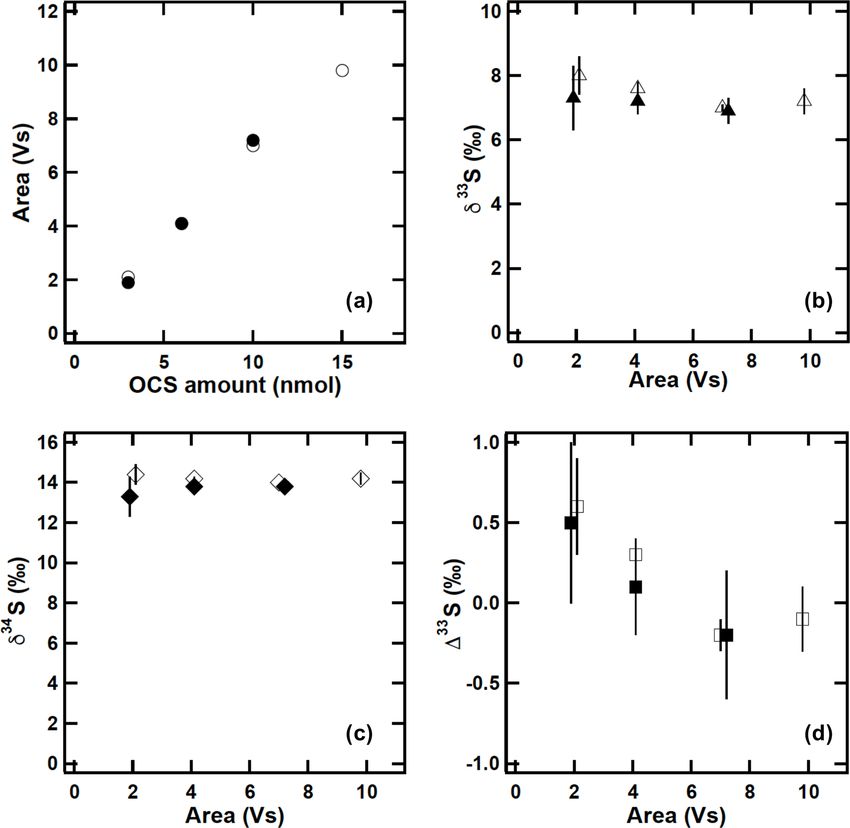
Table 1. OCS samples balanced with He and synthesized OCS sample of averages and standard deviations (1σ ) for sulfur isotope ratios for OCS measured for this study (sampling–
                                          purification system with GC–IR-MS) and with a conventional syringe injection system with GC–IR-MS as described by Hattori et al. (2015).

                                                                                                                                                                                This study                                                                  Modified from Hattori et al. (2015)

www.atmos-meas-tech.net/12/1141/2019/
                                                                                                                              DI–IR-MS                       Syringe injection system with                     Sampling–purification system                 Syringe injection system with GC–
                                                                                                                               (SF6 )a                            GC–IR-MS (S+ )b                                 with GC–IR-MS (S+ )                                  IR-MS (S+ )a
                                                                                                                    n     δ 33 S    δ 34 S   133 S   n          δ 33 S         δ 34 S          133 S   n          δ 33 S         δ 34 S         133 S   n         δ 33 S         δ 34 S       133 S
                                           Sample    Sample type            Concentration      Supplier                            (‰)                                       (‰)                                              (‰)                                             (‰)
                                           A         Commercial cylinder    10.50 %            –                    1    6.5a      12.6a     0.03a   3     6.5 ± 0.2      12.6 ± 0.4      0.03 ± 0.1   –              –              –             –    6   7.3 ± 0.4e     14.3 ± 0.6e    0.0 ± 0.2e
                                                     (balanced with He)                                                 ±0.05      ±0.01     ±0.01
                                           B         Commercial cylinder    5.9 µmol mol−1     –                    –         –         –        –   3    7.0 ± 0.1c     14.1 ± 0.2c     −0.2 ± 0.1c   3     6.9 ± 0.4d    13.8 ± 0.4d    −0.2 ± 0.4d   3   7.3 ± 0.4e     14.3 ± 0.2e    0.0 ± 0.3e
                                                     (balanced with He)
                                           C         Synthesized            100 %              Wako                 –         –         –        –   3   −3.3 ± 0.1d     −6.3 ± 0.2d    −0.06 ± 0.1d   3   −2.8 ± 0.2d     −5.5 ± 0.4d    0.03 ± 0.2d   –             –              –            –
                                                     (CO + S reaction)
                                           D         Synthesized            100 %              Sigma-Aldrich        –         –         –        –   3    1.1 ± 0.2d      2.4 ± 0.2d    −0.07 ± 0.1d   3     1.5 ± 0.4d     2.8 ± 0.7d    0.08 ± 0.1d   –             –              –            –
                                                     (CO + S reaction)
                                                                                                                                                                                                                                                                                                           K. Kamezaki et al.: Measuring 34 S/32 S isotope ratio of carbonyl sulfide

                                           E         Synthesized            100 %              Mixture of Wako      –         –         –        –   3   −1.5 ± 0.1d     −2.5 ± 0.2d     −0.2 ± 0.1d   3   −0.8 ± 0.6d     −1.9 ± 0.6d    −0.2 ± 0.3d   –             –              –            –
                                                     (CO + S reaction)                         and Sigma-Aldrich
                                          a δ 33 S, δ 33 S, and 133 S values of SF chemically converted from OCS in sample A were corrected to values relative to the international standard (VCDT) notation by SF converted from IAEA-S-1(Ag S : δ 33 S = −0.055 ‰, Ono et al., 2007; δ 34 S = −0.30 ‰,
                                                                                   6                                                                                                                              6                          2
                                          Robinson, 1993; and 133 S = −0.100 ‰, Ono et al., 2007), and the standard deviations (1σ ) of the measurements were estimated based on measurements repeated 25 times.
                                          b System developed by Hattori et al. (2015).
                                          c Corrected to values relative to the international standard (VCDT) notation by using sample A measured in this study.
                                          d Corrected to values relative to the international standard (VCDT) notation by using daily sample B injected from the line developed by Hattori et al. (2015).
                                          e Average and precision of δ 34 S(SF ) value chemically converted from OCS in sample A was corrected to values relative to the international standard (VCDT) notation by SF converted from IAEA-S-1(Ag S : δ 33 S = −0.055 ‰ Ono et al., 2007;
                                                                                 6                                                                                                                                   6                             2
                                          δ 34 S = −0.30 ‰, Robinson, 1993; and 133 S = −0.100 ‰ Ono et al., 2007, Hattori et al., 2015).

Atmos. Meas. Tech., 12, 1141–1154, 2019
                                                                                                                                                                                                                                                                                                           1143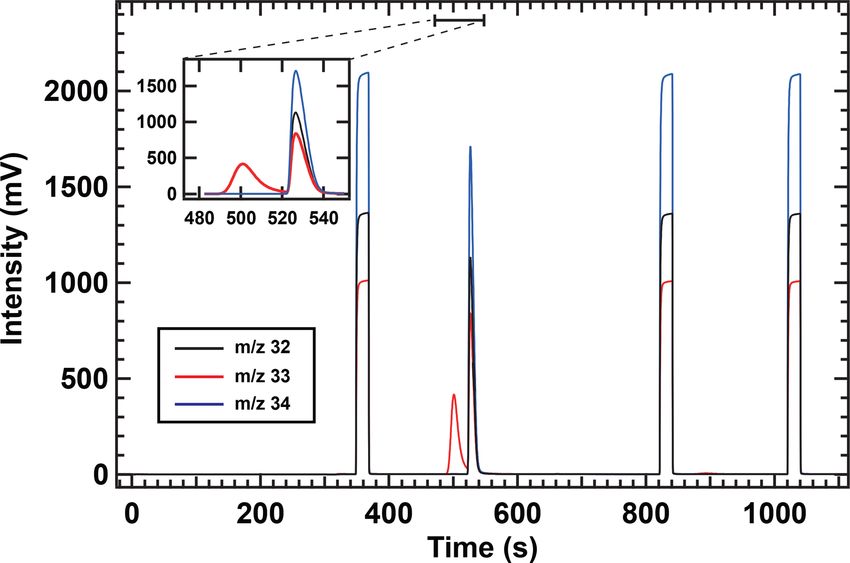
1144                                                                K. Kamezaki et al.: Measuring 34 S/32 S isotope ratio of carbonyl sulfide

Table 2. Sample information for compressed air in cylinders collected at Kawasaki, Japan.

                        Concentration        δ 34 S(OCS)
          Sample          pmol mol−1                    ‰       Experiments                                                               Collecting date
          F                 380 ± 15a         11.7 ± 0.4        Test of collection efficiency                                             25 July 2017
          G                  168 ± 5a         6.1 ± 0.4d        Determination of sulfur isotopic composition                              2 July 2012
          H                  200 ± 7b                  –        Preservation test for OCS amount                                          2 December 2017
          I                371 ± 25b,c         9.5 ± 0.4        Preservation test for OCS amount                                          26 October 2018
          J                 496 ± 30c          9.3 ± 0.4        Preservation test for OCS amount and δ 34 S(OCS) value                    1 December 2018
          K                 460 ± 29c         10.4 ± 0.4        Preservation test for OCS amount and δ 34 S(OCS) value                    26 December 2018
        a Measured using a Q-MS with a picomole-level calibration curve. b Measured using a Q-MS with a nanomole-level calibration curve after sampling.
        c Measured using an IR-MS with a calibration curve in Fig. 4 after sampling with 1σ uncertainty of 6 %. d The previous δ 34 S(OCS) value measured by Hattori
        et al. (2015) was (4.9 ± 0.3) ‰.

                                                                                         (1.9 cm) outer diameter, 50 cm length) with an air inlet at
                                                                                         the side 4 cm below the top and an inner 1/4 in. (0.63 cm)
                                                                                         stainless steel tube (Bahlmann et al., 2011). From top to bot-
                                                                                         tom, the sampling tube package is the following: 0–30 cm,
                                                                                         empty; 30–40 cm, silanized glass beads 2 mm; 40–43 cm,
                                                                                         Tenax TA (60/80 mesh; GL Sciences Inc., Tokyo, Japan);
                                                                                         43–47 cm, Porapak N (80/100 mesh; Sigma-Aldrich Corp.,
                                                                                         Japan); 47–50 cm, empty, and adsorbents separated by plugs
                                                                                         of precleaned glass wools (GL Sciences Inc., Tokyo, Japan).
                                                                                         We developed this sampling tube according to Bahlmann et
                                                                                         al. (2011). Detailed functions of the respective components
                                                                                         are described therein. Briefly, the glass bead traps the remain-
Figure 1. Schematic diagram of the OCS sampling system. Sys-                             ing water vapour from the sampled air and prevents water
tem components: V, valve; pump, vacuum pump; MFC, mass flow                              vapour adsorption on the Tenax TA and Porapak N. The glass
controller.                                                                              bead further increases the temperature exchange between the
                                                                                         cryotrap walls and the sampled air. The Tenax TA and Pora-
                                                                                         pak N can be used for trapping volatile organic compounds.
2.2    Sampling system                                                                   We assume that OCS is sampled on the Tenax TA and Po-
                                                                                         rapak N, but most OCS might be trapped on Tenax TA. Al-
A schematic diagram of the sampling system is depicted in                                though some components might not be necessary for OCS
Fig. 1. The sampling system size and weight are 50 cm ×                                  collections, up to this point, it has been working well for OCS
50 cm × 50 cm (width × height × depth) and 4 kg, except                                  sampling.
for a dewar (37 cm outer diameter, 66 cm height, and 11 kg                                  The adsorption tube consists of a stainless steel tube (with
weight) (MVE SC 20/20; Chart Industries Inc., Georgia,                                   1/4 in. (0.63 cm) outer diameter, 17.5 cm length) filled with
USA). For field campaigns, the system can be easily disas-                               Tenax TA. Before experiments, the sampling tube and the
sembled and transported in two containers of 40 cm × 30 cm                               adsorption tube were conditioned in the laboratory using
× 20 cm (width × height × depth). Reassembling the sam-                                  100 mL min−1 high-purity He flow at 160 ◦ C with an electric
pling system on site can easily be done within 2 h, mak-                                 heating mantle (P-22; Tokyo Technological Labo Co., Ltd.,
ing it suitable for field campaigns. The main compartments                               Kanagawa, Japan) for 6 h and 50 mL min−1 high-purity He
of the sampling system are 1/4 in. (0.64 cm) PTFE tubes,                                 flow at 330 ◦ C with an electric heating mantle (P-25; Tokyo
1/8 in. (0.32 cm) stainless steel tubes, 1/16 in. (0.16 cm)                              Technological Labo Co., Ltd.) for 6 h, respectively. We con-
Sulfinert-treated stainless steel tubes (Restek Corp., PA,                               firmed that possible contamination of OCS in the tubes was
USA), Sulfinert-treated stainless steel ball valves V1, V2,                              less than 10 pmol after conditioning. We also confirmed that
V5, and V9, and stainless steel ball valves V3, V4, V6, V7,                              the surface was inert for at least 3 days and that the inac-
and V8 behind the sampling tube (Fig. 1). Excluding union                                tive state of the surface of adsorbents in these tubes would
tees made of stainless steel immediately before the pump,                                be maintained under a no-leakage condition. It is notewor-
union tees coming in contact with the sampled OCS are made                               thy that conditioning steps would be required if stainless
of Sulfinert-treated stainless steel (Fig. 1).                                           tubes are replaced by Sulfinert-treated tubes/valves because
   The cryotrap sampling tube for OCS concentration from                                 this conditioning was aimed at removing strongly adsorbed
ambient air consists of an outer stainless steel tube (3/4 in.

Atmos. Meas. Tech., 12, 1141–1154, 2019                                                                           www.atmos-meas-tech.net/12/1141/2019/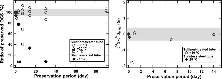
K. Kamezaki et al.: Measuring 34 S/32 S isotope ratio of carbonyl sulfide 1145
volatile organic compounds such as ethanol and acetalde- ing mantle (P-22; Tokyo Technological Labo Co., Ltd.) for
hyde in adsorbents, which might interfere with OCS collec- 30 min at 30 mL min−1 with high-purity He for conditioning.
tion and/or react with OCS. Coil-shaped trap 3 is an empty stainless steel tube (1/16 in.
During sampling, valves V1, V2, V3, and V4 were opened. (0.16 cm) outer diameter, 50 cm length). Coil-shaped trap 4 is
Then atmospheric samples were drawn with a low-volume a fused silica capillary tube (0.32 mm inner diameter, 50 cm
diaphragm pump (LV-40BW; Sibata Scientific Technology length, GL Sciences Inc.). The GC1 (GC-8610T; JEOL Ltd.,
Ltd., Saitama, Japan) through the sampling system with Tokyo, Japan) is equipped with a column packed with Po-
a flow of (5.00 ± 0.25) L min−1 . The air was first passed rapak Q (80/100, GL Sciences Inc.) (1/8 in. (0.32 cm) outer
through a membrane filter (47 mm diameter, 1.2 µm pore, diameter, 3 m length) to separate OCS from CO2 . The GC1
Pall Ultipor N66 sterilizing-grade filter; Pall Corp., New oven temperature for OCS purification was programmed to
York, USA) set in a NILU filter holder system (70 mm di- provide 30 ◦ C for 5 min, increasing to 60 ◦ C at 30 ◦ C min−1 ,
ameter, 90 mm length: Tokyo Dylec Corp., Tokyo, Japan) to followed by an increase to 230 ◦ C at 30 ◦ C min−1 starting
remove atmospheric aerosol. Then it was directed through a 40 min after the start of the program for GC1, and 230 ◦ C for
condenser (EFG5-10; IAC Co. Ltd., Japan) kept at approxi- 1 min.
mately −15 ◦ C to remove water vapour from the air. The air After the adsorption tube containing OCS was connected
was then passed through the sampling tube at temperatures of to the purification system, v3, v4, and v5 (Fig. 2) were
−140 to −110 ◦ C by vapour of the liquid N2 in a dewar. The opened and the air in the line was pumped out using a rotary
OCS was enriched in the sampling tube, whereas other main pump (DA-60D; Ulvac Kiko, Miyazaki, Japan) for 5 min; v3,
gases (N2 , O2 , Ar, etc.) were passed through the sampling v4, and v5 (Fig. 2) were then closed. When the adsorption
tube. tube was heated at 130 ◦ C and v2, v7, v8, and v6 (Fig. 2)
After sampling, valves V1 and V4 were closed, and valves were opened, gases in the adsorption tube passed through
V5, V6, V7, and V8 were opened. Then, the sampling trap 1 cooled by dry ice (−78 ◦ C) to remove trace remnant
tube was removed carefully from the dewar manually and water vapour. Also, OCS was collected in trap 2, with Tenax
was heated gradually to 130 ◦ C. The vaporised gases in the TA cooled by dry ice–ethanol (−72 ◦ C) with a high-purity
sampling tube were passed to the adsorption tube cooled He flow rate of 30 mL min−1 . After 15 min, port valve (PV)
at −78 ◦ C using dry ice–ethanol after removal of the re- 1 was changed. Trap 2 was then removed from dry ice–
maining water vapour by a Nafion dryer (MD-110-96S; ethanol and was heated at 130 ◦ C. The retention times of CO2
Perma Pure LLC, NJ, USA). The flow rate was regulated and OCS were initially determined by injecting a mixture of
(approx. 50 mL min−1 ) by a needle valve equipped with a 8 mmol of CO2 from pure CO2 in a cylinder (99.995 % pu-
flow meter for 20 min. After the flow rate became lower rity; Japan Fine Products Co. Ltd.) and 10 nmol of OCS from
than 10 mL min−1 , V4 was opened. The sampling tube was sample C. They were 3–10 min for CO2 and 20–30 min for
flushed with pure N2 (> 99.99995 vol. %) at 50 mL min−1 for OCS at a flow rate of 25 mL min−1 . Trap 3 was cooled by
40 min. After the transfer of samples, V6, V7, and V8 were liquid N2 starting 10 min after the start of the program for
closed. Then OCS was preserved in the adsorption tube. We GC1; PV2 was changed from 15 to 35 min after injection of
initially confirmed that OCS did not pass through an adsorp- samples to GC1 to introduce OCS to trap 3. OCS with high-
tion tube at a flow rate lower than 50 mL min−1 using two purity He was passed through the column and collected in
adsorption tubes connected in series from the second adsorp- trap 3 for 20 min. After OCS collection in trap 3, the OCS
tion tube: OCS was observed only from the first tube, not was again transferred to trap 4 in liquid N2 at 6 mL min−1
from the second tube. For this study, the collected OCS sam- by high-purity He with removal of liquid N2 from trap 3 to
ples in adsorption tubes were measured within 30 min, except a cryofocus. Trap 4 was then removed from liquid N2 ; the
for the preservation test. OCS passed through the GC2 and was introduced directly to
the detectors (quadrupole mass spectrometer (Q-MS) or IR-
2.3 Purification system MS depending on the experiments explained below).
After sampling OCS from the air using the sampling system 2.4 Determination of the OCS concentration
as described above, the collected OCS was purified and con-
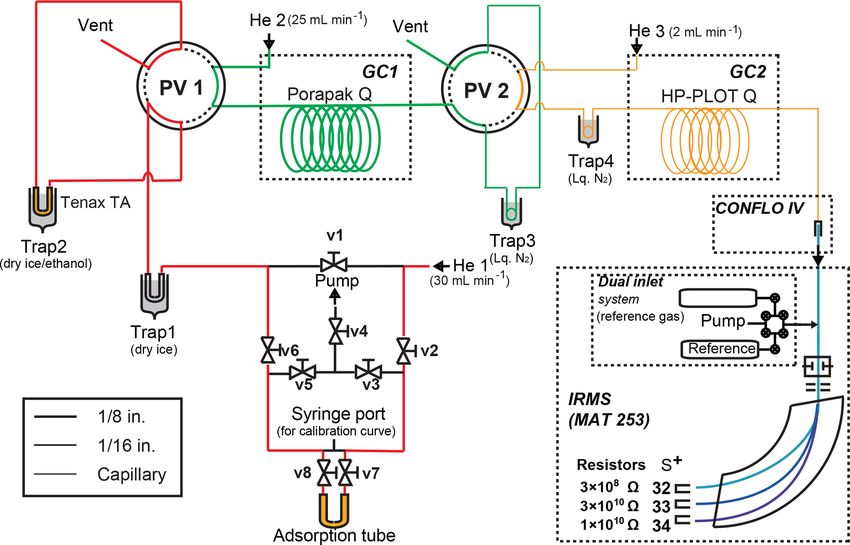
nected directly to the measurement system. The schematic The OCS concentrations were measured with a GC–Q-MS
system is shown in Fig. 2. Excluding a fused silica capil- (7890A; Agilent Technologies Inc., CA, US, coupled to Q-
lary tube, all tubes and valves are made of stainless steel. MS, 5975C; Agilent Technologies Inc., CA, USA) equipped
U-shaped trap 1 is a 50 cm, 1/4 in. (0.64 cm) outer diame- with a capillary column (0.32 mm inner diameter, 25 m
ter (1/8 in. (0.32 cm) inner diameter) stainless steel tube. U- length, and 10 µm thickness; HP-PLOT Q, Agilent Technolo-
shaped trap 2 is a 30 cm, 1/8 in. (0.32 cm) outer diameter gies, CA, USA). The He flow was set to 1.5 mL min−1 and
(1/16 in. (0.16 cm) inner diameter) stainless steel tube filled the oven temperature program was set as 60 ◦ C for 15 min,
with Tenax TA (60/80 mesh; GL Sciences Inc.). Before the increased to 230 ◦ C at 60 ◦ C min−1 , and then held at 230 ◦ C
experiment, trap 2 is heated to 150 ◦ C by an electric heat- for 1 min.
www.atmos-meas-tech.net/12/1141/2019/ Atmos. Meas. Tech., 12, 1141–1154, 2019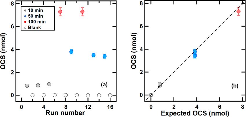
1146                                              K. Kamezaki et al.: Measuring 34 S/32 S isotope ratio of carbonyl sulfide

Figure 2. Schematic diagram of the OCS purification system. System components: V, valve; pump, vacuum pump; MFC, mass flow con-
troller.

   To ascertain the OCS concentration of sample A once a          trations for samples F and G were measured within at least a
month, and to ascertain the collected OCS amounts using a         week before or after the experiment. In a similar manner, the
sampling system, we made a calibration curve for OCS rang-        cylinders of samples H, I, J, and K were used for experiments
ing from 0.1 nmol to 10 nmol using a Q-MS. The calibration        within 2–3 days. Therefore, a change in OCS concentration
curve for the nanomole level is calculated with an injection      in samples might occur.
of sample B with a volume of 0.5, 2.2, 4.4, 8.8, 11, 13.2,
17.6, 22, and 44 mL (n = 3). The precision (standard devia-       2.5   Determination of the sulfur isotope ratios of OCS
tion (1σ ) relative to mean) of the OCS amount from a syringe
injection was estimated to be ±3 % by the standard deviation
of the relative error between the measured values and the es-     For determination of the sulfur isotope ratios of OCS, OCS
timated value for calibration curves.                             was passed through the GC2 after a purification system as de-
   To ascertain the OCS concentrations of samples F and G,        scribed above. Then it was introduced directly to the IR-MS
we prepared calibration curves for OCS ranging from 0 to          (MAT253; Thermo Fisher Scientific Inc., Berlin, Germany)
100 pmol using a Q-MS. The calibration curve for the pico-        via an open split interface (ConFlo IV; Thermo Fisher Sci-
mole level is calculated from an injection of sample B with       entific Inc.). Reference OCS of sample A was purified with
a volume of 0, 200, 400, and 800 µL (n = 3) with a preci-         liquid N2 (−196 ◦ C) and then introduced via a conventional
sion of ±3 % as estimated similarly above. For determina-         dual inlet system. Pure OCS is not commercially available
tion of OCS concentrations of samples F and G, samples            in Japan because of its toxicity (Hattori et al., 2015). In ad-
F and G were stored in 50 mL two-neck glass bottles with          dition to the method introducing OCS to the IR-MS as de-
atmospheric pressure and were introduced to the purifica-         scribed above, the conventional syringe injection line, which
tion system from an attached glass bottle instead of an ad-       was previously used for Hattori et al. (2015) and Kamezaki
sorption tube. The measured OCS concentrations for sam-           et al. (2016), was also used for comparison or calibration.
ples F and G were, respectively, (380 ± 15) pmol mol−1 and        Briefly, the syringe-injected OCS was collected in stainless
(160 ± 5) pmol mol−1 (Table 2).                                   steel tubes (10.5 mm inner diameter, 150 mm length) cooled
   The OCS concentrations for samples F, G, H, and I were         at −196 ◦ C by liquid N2 with a gentle vacuum by a rotary
lower than typical atmospheric OCS concentrations (400–           pump (Pascal, 2010; Pfeiffer Vacuum GmbH, Aßlar, Ger-
550 pmol mol−1 ) (Montzka et al., 2007), even though the          many) with regulation using a valve. After transfer of OCS
samples were compressed air collected from the ambient at-        to the trap, the two-way six-port valve was changed. Then
mosphere. Because we were concerned about the changes in          liquid N2 was removed from the trap. Subsequently, OCS
OCS concentrations for samples F and G, the OCS concen-           was transferred and collected in a fused silica capillary tube
                                                                  (0.32 mm inner diameter, 50 cm length; GL Sciences Inc.)

Atmos. Meas. Tech., 12, 1141–1154, 2019                                             www.atmos-meas-tech.net/12/1141/2019/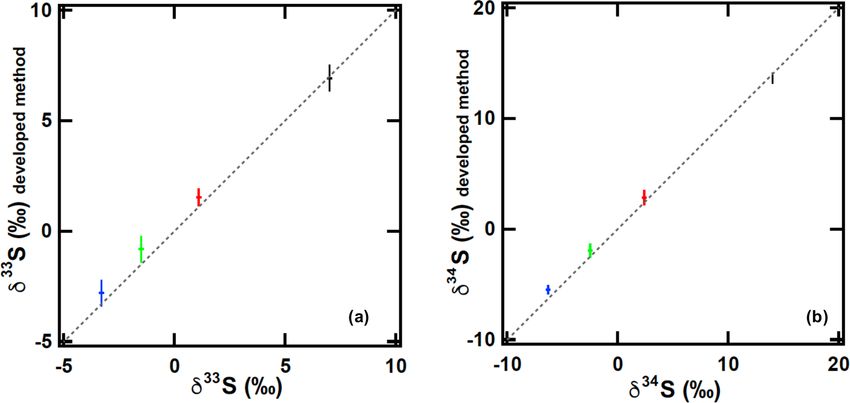
K. Kamezaki et al.: Measuring 34 S/32 S isotope ratio of carbonyl sulfide                                                       1147

covered by a stainless steel tube containing liquid N2 for
13 min before being introduced into the GC–IR-MS system.
   In the IR-MS ion source, electron impact ionization of
OCS produced S+ fragment ions. The sulfur isotope ratios in
OCS were therefore determined by measuring the fragment
ions 32 S+ , 33 S+ , and 34 S+ using triple Faraday collector
cups. The typical precisions (1σ ) of the replicate measure-
ments (n = 3) are 0.4 ‰, 0.2 ‰, and 0.3 ‰ for δ 33 S(OCS),
δ 34 S(OCS), and 133 S(OCS) values, respectively. A refer-
ence OCS gas was introduced for 20 s three times starting
at t = 350, 825, and 1025 s. The reference gas at t = 350 s
                                                                  Figure 3. OCS sampling using sample F of (380 ± 15) pmol mol−1
was used as the reference for all calculations of OCS sulfur
                                                                  with different sampling times of blank (0 min), 10, 50, and 100 min.
isotope ratios. To remove hydrogen sulfide and ethane from        (a) Collected OCS amounts as a function of run numbers. (b) Ob-
ambient samples, from t = 300 s, the effluent from the GC         served OCS amounts and OCS amounts calculated using OCS con-
column was kept off the MS line using back-flushed helium         centration multiplied by the sampling time. The error bar shows
flow. Sulfur isotope ratios are typically reported as             ±3 % based on the residual of measured OCS peak area and cali-
                                                                  brated OCS peak area. The dotted line shows the slope of x = y.
δ x S = x Rsample /x Rstandard − 1,                        (1)

where x R represents the isotopic ratios (x S/32 S, where x =
                                                                  3     Results and discussion
33 or 34) of the samples and standards. The sulfur isotope
ratios are reported relative to the Vienna Canyon Diablo          3.1    Sampling efficiency of OCS
Troilite (VCDT, quoted as per mil values (‰)). In addition
to the δ values, capital delta notation (133 S value) is used     To test the sampling and desorption efficiency, the cylin-
to distinguish mass-independent fractionation (MIF; or non-       der containing sample F was connected to a flow meter and
mass-dependent fractionation) of sulfur, which causes devia-      the flow was adjusted to 6 L min−1 with a needle valve. An
tion from the mass-dependent fractionation (MDF) line. The        amount of 5 L min−1 was drawn through the sampling sys-
133 S value describes the excess or deficiency of 33 S relative   tem with a pump and the remainder was vented into the
to a reference MDF line. It is expressed as                       air to maintain atmospheric pressure at the sampling inlet.
                                                                  The samples were collected within 2 days to prevent OCS
133 S = δ 33 S − [(δ 34 S + 1)0.515 − 1].                  (2)
                                                                  loss in the cylinder. The vent flow was measured with a
The δ values in this study were determined using the follow-      flow meter (ACM-1A; Kofloc, Tokyo, Japan). To ascertain
ing processes. First, we ascertained the δ 34 S value of sample   the trapping efficiency OCS was sampled for 10, 50, and
A by converting OCS to SF6 . The δ 34 S(SF6 ) value was mea-      100 min with blank test intervals as presented in Fig. 3a (see
sured relative to the VCDT scale by comparing SF6 similarly       Sect. 2.2 for sampling procedure). The sampling times corre-
converted from IAEA-S-1 (Ag2 S: δ 34 S = −0.30 ‰; Robin-          sponded to sampling volumes of (50 ± 2.5) L, (250 ± 13) L,
son, 1993) as described by Hattori et al. (2015). The mea-        and (500 ± 25) L and the corresponding OCS amounts were
sured δ 34 S value of sample A was 12.6 ‰, which was lower        (0.77±0.04) nmol, (3.9±0.2) nmol, and (7.7±0.4) nmol re-
than the data presented by Hattori et al. (2015) with 14.3 ‰      spectively (Fig. 3a).
(Table 1). Secondly, the δ 34 S value of sample B, which was         Recovery and precision (1σ ) for OCS amounts col-
used as a working standard for δ 34 S measurements, was as-       lected for sampling times of 10, 50, and 100 min were
certained from comparison with the δ 34 S value (at VCDT          (0.9±0.1) nmol (n = 3), (3.6±0.2) nmol (n = 3), and (7.4±
scale) of sample A with the GC–IR-MS method using a S+            0.3) nmol (n = 2), respectively. The OCS blanks were
fragment ion. The δ 34 S(OCS) value of sample B in this study     smaller than 15 pmol. These results indicate that the yield
was (14.1 ± 0.2) ‰ (Table 1), showing no significant differ-      of OCS during sampling and transferring from the sampling
ence with the δ 34 S(OCS) value of sample B (14.3 ± 0.2) ‰        tube to the adsorption tube is almost over 95 %. The memory
in data presented by Hattori et al. (2015). It is noteworthy      effect of the system between the sampling runs is expected to
that we also found that the OCS concentration in sample           be less than 1 % when sampling OCS amounts over 3 nmol
B was not changed. Sample B was used as the daily work-           (approx. 50 min). Figure 3b presents a comparison of OCS
ing standard for GC–IR-MS measurement to ascertain sam-           amount between observed OCS amounts and OCS amounts
ple δ 34 S(OCS) values for other samples used throughout this     calculated based on OCS concentration in sample F and sam-
study (Table 1).                                                  pling time, showing that all results fall on the 1 : 1 line. This
                                                                  suggests that almost 100 % of OCS for sampling runs was
                                                                  collected in the sampling tube and was transferred success-
                                                                  fully to the adsorption tube. Although the collected OCS

www.atmos-meas-tech.net/12/1141/2019/                                                Atmos. Meas. Tech., 12, 1141–1154, 2019
1148 K. Kamezaki et al.: Measuring 34 S/32 S isotope ratio of carbonyl sulfide
amount in 10 min was slightly larger than the expected OCS
amount, the OCS amounts in 100 min were slightly lower
than the expected OCS amount. This result indicates that a
small OCS contamination during the sampling and a purifi-
cation system might exist but that it might not be significant,
as discussed above.
3.2 Accuracy of the sulfur isotopic analysis of OCS via
sampling–purification systems
In the developed system, the possibility exists that OCS is
lost by passing OCS through GC1. Also, because the flow
rate of approximately 50 mL min−1 was lower than the flow
rate of approximately 200 mL min−1 reported by Hattori et
al. (2015), the possibility exists that OCS was lost by trap 1.
Therefore, to assess these possibilities, the following test was
conducted. Firstly, 5 nmol of OCS was injected to a system
consisting of trap 2, GC2, and trap 4 and measured as a true
value. Then the same amount of OCS was introduced into
the developed purification system and the amount of OCS
obtained was compared to the true value. These tests re-
Figure 4. OCS amounts and sulfur isotope ratios of differ-
vealed an OCS loss of less than 2 % using a newly developed
ent amounts of OCS injections ascertained using the developed
method and suggest a complete recovery of OCS within the
sampling–purification system and conventional syringe injection
given limits of uncertainty (±3 %). To assess the dependence system (Hattori et al., 2015): (a) OCS amount; (b) δ 33 S; (c) δ 34 S;
of the sulfur isotopic measurements on the OCS amount, dif- (d) 133 S; closed symbols, sampling–purification system developed
ferent amounts of OCS using sample B were tested. We in- for this study; open symbols, conventional syringe injection system.
troduced aliquots of 3, 6, 10, and 15 nmol of sample B over All sulfur isotope ratios are relative to VCDT. The error bars are 1σ
30 min with a gas-tight syringe via a syringe port made from of the measurements based on triplicated measurements.
a tee union with a septum. The syringe port was placed be-
tween the inlet filter and the condenser and the sampling in-
let was connected to high-purity N2 (99.99995 vol. %; Nissan sized OCS (samples B, C, D, and E) with triplicate injec-
Tanaka Corp., Saitama, Japan) (Fig. 1). For each experiment, tions. In Fig. 5, the δ 34 S(OCS) values measured using the
a total volume of 500 L N2 was processed. The OCS contam- developed sampling–purification system were 0.2 ‰ lower
ination for this experiment was (0.30 ± 0.16) nmol (n = 3) (sample B) but 0.8 ‰, 0.4 ‰, and 0.6 ‰ higher (samples C,
when we flushed with 500 L of pure N2 . For comparison, D, and E, respectively) than those measured using the sy-
similar amounts of OCS were also injected using a syringe ringe injection system of Hattori et al. (2015) (Table 1). This
injection system developed previously (Hattori et al., 2015). phenomenon was observed similarly for the δ 33 S(OCS) val-
Comparisons of OCS concentrations and δ and 1 values are ues (Fig. 5c), indicating that this process is not isotopic frac-
depicted in Fig. 4. Although the observed OCS isotope ratios tionation but rather suggests contamination during the sam-
using 3 nmol of OCS with the developed method were scat- pling processes. When considering (0.30 ± 0.16) nmol OCS
tered (1σ uncertainty: 1.0 ‰, 1.0 ‰, and 0.5 ‰, respectively, (i.e. approx. 4 % for 8 nmol OCS samples) with δ 34 S of
for δ 33 S(OCS), δ 34 S(OCS), and 133 S(OCS) values), the re- 3 ‰–18 ‰ covering the reported δ 34 S range of OCS sources
producibilities at the 6 nmol level were sufficient (1σ uncer- (Newman et al., 1991), the accuracy of the δ 34 S(OCS) can
tainty: 0.4 ‰, 0.2 ‰, and 0.4 ‰, respectively, for δ 33 S(OCS), be shifted from −0.3 ‰ to +0.3 ‰. Because the precision of
δ 34 S(OCS), and 133 S(OCS) values) and were similar to 1σ uncertainty is 0.2 ‰, the overall precision values (1σ ) for
those obtained with the conventional syringe injection sys- δ 34 S of this sampling–purification system were estimated as
tem for Hattori et al. (2015) (Fig. 4). Consequently, this sys- 0.4 ‰.
tem better accommodates OCS samples over 6 nmol, indi-
cating the necessity for collection of ambient air in amounts 3.3 Sulfur isotope ratio for atmospheric OCS
greater than 300 L.
Furthermore, to test possible sulfur isotopic fractiona- Four ambient air samples were collected at the Suzukakedai
tions during sampling–purification processes, which might campus of the Tokyo Institute of Technology located in
change the measurement accuracy, we compared the devel- Yokohama, Japan (35.5◦ N, 139.5◦ W, 27 m height), dur-
oped sampling–purification system with the conventional sy- ing 23–25 April 2018 every 12 h (sampling times were
ringe injection system using 8 nmol of the in-house synthe- 23 April 2018 at 12:00 JST, 24 April 2018 at 00:00,
Atmos. Meas. Tech., 12, 1141–1154, 2019 www.atmos-meas-tech.net/12/1141/2019/K. Kamezaki et al.: Measuring 34 S/32 S isotope ratio of carbonyl sulfide 1149
Figure 5. Sulfur isotope ratios (a δ 33 S and b δ 34 S) ascertained from
the developed sampling–purification system (y axis) and conven-
tional syringe injection system (Hattori et al., 2015) (x axis). OCS
sample amounts are 8 nmol. Different colours represent different
samples: black, sample B; red, sample C; green, sample D; blue, Figure 7. IR-MS chromatogram of atmospheric samples collected
sample E. The dotted line shows the slope x = y. The error bar is at the Suzukakedai campus of the Tokyo Institute of Technology.
1σ of each amount of triplicated OCS injection. Liquid N2 removal from trap 4 occurred at 0 s in the purification
system. Reference OCS was injected three times starting at 350,
825, and 1025 s for 20 s.
and m/z 34. The interfering compound could have not yet
been identified. Known fragments interfering on m/z 33 are
CH5 O+ originating from the protonation of methanol and/or
the reaction of CH3 O+ with H2 O, CH2 F+ that is indicative of
hydrofluorocarbons, and/or NF+ deriving from nitrogen tri-
fluoride (NF3 ). To measure m/z 33 of OCS without interfer-
ences, further improvement of peak separation of OCS with
interferences is required by changing the parameter of the
separation in the system and/or data processing. For example,
Figure 6. OCS concentrations and δ 34 S(OCS) values for atmo-
a custom-made MATLAB routine, which can extrapolate the
spheric samples collected at the Suzukakedai campus of the Tokyo peak tail of interference via an exponentially decaying func-
Institute of Technology located in Yokohama, Japan. The error bar tion to distinguish the two gaseous species as described in
is 6 % for OCS concentration based on the precisions of syringe Zuiderweg et al. (2013), would enable us to analyse m/z 33
injection and flow rate of the diaphragm pump in the sampling sys- in addition to the standard ISODAT software used for isotope
tem. The precision of δ 34 S is estimated from a 1σ uncertainty of ratio measurements.
0.4 ‰. The observed OCS concentrations for atmospheric sam-
ples were 447–520 pmol mol−1 (Fig. 6a), averaging (492 ±
34) pmol mol−1 . Data show no clear differences between
24 April 2018 at 12:00, and 25 April 2018 at 00:00). The 00:00 and 12:00 in 2 days (p value = 0.65). This OCS con-
sampling volume was 500 L (i.e. 100 min with a pump flow centration observed at the Suzukakedai campus shows good
of 5 L min−1 ). Measurements of OCS concentrations and sul- agreement with the OCS concentrations observed at a simi-
fur isotope ratios were carried out within 30 min after the lar latitude in the US (e.g. 400–550 pmol mol−1 ; Montzka et
sampling. The time for a single measurement of δ 34 S value al., 2007). Berkelhammer et al. (2014) reported diurnal vari-
for atmospheric OCS was 100 min (500 L) for sampling of ation for OCS concentrations in the US with the lowest at
air, 40 min for transferring to the adsorption tube, 40 min for 08:00 and the highest at 16:00 with 80 pmol mol−1 changes
purification, and 20 min for measurement using an IR-MS. in a day. Moreover, the differences of OCS concentrations
The OCS concentrations and δ 34 S(OCS) values observed for for four atmospheric samples were less than 80 pmol mol−1 .
ambient air are presented in Fig. 6. The observed δ 34 S(OCS) values of four atmospheric samples
In contrast to the δ 34 S(OCS) value, the δ 33 S(OCS) value were 10.4 ‰–10.7 ‰ (Fig. 6b) and averaged (10.5 ± 0.4) ‰.
in air was not determined because of the unexpected peak The δ 34 S(OCS) values also showed no clear diurnal differ-
(approx. 40 mV height) observed for m/z 33, which slightly ence (p values = 0.29) (Fig. 6b). Given the diurnal OCS vari-
overlapped the OCS peak of the chromatogram (Fig. 7). ations, some future study is clearly necessary to ascertain
We notably did not observe any interferences on m/z 32 whether or not δ 34 S(OCS) values have diurnal variations by
www.atmos-meas-tech.net/12/1141/2019/ Atmos. Meas. Tech., 12, 1141–1154, 20191150 K. Kamezaki et al.: Measuring 34 S/32 S isotope ratio of carbonyl sulfide
comparing δ 34 S(OCS) values for the highest OCS concentra- this fact requires appropriate ways of preservation of OCS
tion at 08:00 and the lowest OCS concentration at 16:00. during transportation from field sampling sites to laboratory
It is noteworthy that the δ 34 S(OCS) values of four at- until analysis.
mospheric samples were clearly distinct from our earlier In order to minimize potential OCS decomposition on the
observed δ 34 S(OCS) value of (4.9 ± 0.3) ‰ obtained from surface wall, we modified the adsorption tube by replacing
sample G (Hattori et al., 2015), which was postulated as a the stainless steel tube and valves with a Sulfinert-treated
global representative δ 34 S(OCS) value in the atmosphere. tube and Sulfinert-treated valves. The preservation of OCS
In fact, the OCS concentrations in the commercial cylin- on the modified adsorption tubes at different storage tem-
ders F, G, and H were significantly lower than typical at- peratures was investigated using samples H, I, J, and K.
mospheric OCS concentrations of approximately 500 nmol The samples were processed as that described in Sect. 2.2
mol−1 (Table 2). Ascertaining the δ 34 S(OCS) value in sam- and transferred to the adsorption tubes. The adsorption tubes
ple G using the current sampling–purification system yielded were stored at temperatures of 25, 4, −20, and −80 ◦ C until
a δ 34 S(OCS) value of (6.1 ± 0.2) ‰ slightly higher than the measurements. After each storage period, the samples were
previous value of (4.9±0.3) ‰ (Hattori et al., 2015). It is pos- analysed for OCS yields and δ 34 S(OCS) values as described
sible to explain this 1.2 ‰ increase for the δ 34 S(OCS) value in Sect. 2.3, 2.4, and 2.5. A rapid OCS decomposition of ap-
for a case in which the contaminated OCS has a δ 34 S(OCS) proximately 20 % during 7 days of storage was observed for
value of over 17 ‰. However, such a high δ 34 S(OCS) value the stainless steel adsorption tubes stored at 25 ◦ C. A sim-
from contamination requires a situation in which the con- ilar pronounced loss was observed for the Sulfinert-treated
taminated OCS comes only from the ocean, which is not adsorption tubes stored at 4 ◦ C but at a storage temperature
likely. Because the atmospheric δ 34 S(OCS) values in this of −20 ◦ C. The OCS was stable for 30 days at −20 ◦ C and
study were (10.5 ± 0.4) ‰ and higher than that for sample for at least 90 days at −80 ◦ C within a 1σ uncertainty of 6 %
G, the increased δ 34 S(OCS) values are expected to be af- (Fig. 8a). Furthermore, we found that the δ 34 S(OCS) values
fected by isotopic fractionation during OCS degradation in showed no significant change during storage for at least 14
the cylinder and not by contamination. The causes for the days at −80 ◦ C (Fig. 8b). These results demonstrate that it is
OCS losses in the commercial pressurized air cylinders could possible to apply this method for field campaigns by storing
not be investigated here. Indeed, as reported by Kamezaki the adsorption tube at −80 ◦ C after sampling.
et al. (2016), OCS is decomposed by hydrolysis, which in-
creases the δ 34 S(OCS) value. Additionally, observation of 3.5 Atmospheric implications
OCS loss caused by adsorption to walls in the canister was re-
ported by Khan et al. (2012). The compressed air of samples The δ 34 S(OCS) value of (10.5 ± 0.4) ‰ is generally consis-
F and G might be affected by anthropogenic OCS sources at tent with earlier estimation by Newman et al. (1991), who
the sampling site and/or during the compressing processes. expected the mean δ 34 S(OCS) values of 11 ‰ based on the
All in all, the δ 34 S(OCS) value of sample G is no longer con- flux of continental emission to be 3 ‰ and oceanic emission
sidered to be a representative of atmospheric OCS. to be 18 ‰ (Newman et al., 1991). This estimation is based
on older information, but current measurements of atmo-
3.4 Preservation tests spheric dimethyl sulfide (DMS) and dimethylsulfonioproion-
ate (DMSP) are similar to 18 ‰ (Said-Ahmad and Amrani,
As described above, we measured OCS concentration and 2013; Amrani et al., 2013; Oduro et al., 2012); continental
sulfur isotope ratio of atmospheric samples within 30 min af- sulfur sources also show approximately 0 ‰–5 ‰ (Tcherkez
ter sampling. The OCS concentrations are consistent with the and Tea, 2013).
observed OCS concentrations in the same latitude and our It is noteworthy that the potential importance of tropo-
tests revealed no OCS losses under these conditions. How- spheric sulfur isotopic fractionations during OCS sinks. To
ever, after the development of the system, we realized up to date, sulfur isotopic fractionations were reported as −5 ‰ to
50 % of OCS can be decomposed during storage of the ad- 0 ‰ for reaction with OH radical (Schmidt et al., 2012) and
sorption tube after we have measured the samples within 14 −2 ‰ to −4 ‰ for decomposition by soil microorganisms
days after sampling (Fig. 8a). We also found that the OCS in (Kamezaki et al., 2016; Ogawa et al., 2017). Sulfur isotopic
the stainless steel adsorption tubes stored at 25 ◦ C showed fractionation for OCS by plant uptake, the dominant OCS
only slight changes in concentration with (−6 ± 6) % and sink in the troposphere (Berry et al., 2013), has not been de-
(0.2 ± 0.4) ‰ for δ 34 S(OCS) values after 3 h (Fig. 8b). All termined, but the theoretical isotopic fractionation constant
data sets presented up to this point were undertaken immedi- by plant uptake is −5.3 ‰ (Angert et al., 2019). Therefore,
ately after the sampling (i.e. shorter than 30 min). Therefore, all sulfur isotopic fractionation constants by OCS degrada-
we did not expect marked changes in OCS concentrations tion are negative, indicating that the δ 34 S(OCS) values can
and the δ 34 S(OCS) values for most datasets including atmo- be increased by OCS degradation in the troposphere. Be-
spheric OCS samples. Because OCS is known to react with cause the main OCS sink is photosynthesized by plants, the
the surface of stainless steel (Khan et al., 2012), for future use δ 34 S(OCS) values in the atmosphere might be increased in
Atmos. Meas. Tech., 12, 1141–1154, 2019 www.atmos-meas-tech.net/12/1141/2019/K. Kamezaki et al.: Measuring 34 S/32 S isotope ratio of carbonyl sulfide 1151 Figure 8. (a) Changes in OCS concentrations preserved in the OCS storage test in adsorption tubes at different temperatures and tubes. (b) Changes in δ 34 S(OCS) preserved in the OCS storage test. The shaded bar shows ±6 % for OCS concentration and ±0.4 ‰ for the δ 34 S(OCS) value based on the precisions of syringe injection and the flow rate of the diaphragm pump in the sampling system. the growing season for plants in April. However, because of ments, to elucidate OCS in the troposphere and its relation the long lifetime of OCS, δ 34 S(OCS) values might not be to biochemical activity by plant and soil microorganisms, sensitive to seasonal variation. Future studies must be con- OCS sulfur isotope analysis provides a new tool to investi- ducted to determine the isotopic fractionation constants and gate soil OCS sinks in the troposphere. To date, we have de- observations of δ 34 S(OCS) values to estimate the dynamics termined the isotopic fractionation constants for OCS under- of atmospheric δ 34 S(OCS) values in the troposphere. going bacterial OCS degradation and its enzyme (Kamezaki In addition to our observation of atmospheric δ 34 S(OCS) et al., 2016; Ogawa et al., 2017). Similarly, additional studies values with (10.5±0.4) ‰ at the Suzukakedai campus, Yoko- that include specific examination of isotopic fractionation by hama, Japan, δ 34 S(OCS) values of (13.4±0.5) ‰ in August– plant uptake, another major sink of atmospheric OCS, are in- October at Israel, (12.8 ± 0.5) ‰ in February–March in Is- dispensable for distinguishing the respective OCS fluxes of rael, and (13.1±0.7) ‰ in February–March at the Canary Is- soil and plants. By coupling isotopic fractionations by soil lands, Spain, were recently reported using the GC–MC–ICP- and plant with atmospheric observations of δ 34 S(OCS) val- MS method (Angert et al., 2019). These differences indicate ues using our newly developed method, the atmospheric ob- that the atmospheric δ 34 S(OCS) values might not be homo- servations of δ 34 S(OCS) values are expected to help refine geneous, instead reflecting some geographic effects and/or estimates of biological activities of plant and soil microor- potential difference for isotopic fractionations during sink ganisms and their respective contributions to OCS degrada- processes. Given the higher influences of sulfur isotopic frac- tion in the troposphere. tionations on δ 34 S(OCS) values during growing seasons, it is not likely to explain lower atmospheric δ 34 S(OCS) val- 3.6 Comparison with other methods ues for the Suzukakedai campus in April compared to those for Israel and the Canary Islands observed in February– Here we discuss the comparison of this sampling system March. Rather, δ 34 S(OCS) values of (10.5 ± 0.4) ‰ at the coupled with the GC–IR-MS and GC–MC–ICP-MS meth- Suzukakedai campus might be more affected by anthro- ods (Said-Ahmad et al., 2017; Angert et al., 2019). The re- pogenic OCS emission and/or less affected by oceanic OCS quired sample amounts for our IR-MS system were over emissions compared to the samples collected in Israel or the 6 nmol OCS. The overall precision value (1σ ) for the at- Canary Islands with higher δ 34 S(OCS) values. Potential an- mospheric δ 34 S(OCS) value is 0.4 ‰. By contrast, the GC– thropogenic OCS sources are Chinese emissions from rayon MC–ICP-MS method (Said-Ahmad et al., 2017; Angert et production (rayon yarn and staple rayon) and coal (indus- al., 2019) has a similar precision of 0.6 ‰ but only requires try and residential emissions), as pointed out by recent OCS 20 pmol of OCS. Consequently, the IR-MS method requires source inventories (Zumkehr et al., 2018). In fact, the OCS an OCS sample 300 times larger than that for the GC–MC– concentration in the vicinity of China is high based on satel- ICP-MS method. Therefore, our IR-MS method with a devel- lite observation (Glatthor et al., 2015). Future study is neces- oped large-volume air sampling system has shortcomings for sary to observe spatial and temporal variation of δ 34 S(OCS) sample size and/or logistics for field campaigns. However, it values to discuss the link between anthropogenic activity and is worth noting that benefits of our IR-MS method with its OCS cycles. large-volume air sampling system include its potential appli- In addition to tropospheric OCS sources, OCS has some cation of multi-isotope measurements of OCS by measuring potential as a tracer of net ecosystem exchange into GPP on CO+ fragment ions for carbon and oxygen isotopes as well land (Campbell et al., 2008). Based on our earlier experi- as S+ fragment ions. www.atmos-meas-tech.net/12/1141/2019/ Atmos. Meas. Tech., 12, 1141–1154, 2019
1152                                                   K. Kamezaki et al.: Measuring 34 S/32 S isotope ratio of carbonyl sulfide

4   Summary                                                           Supplement. The supplement related to this article is available
                                                                      online at: https://doi.org/10.5194/amt-12-1141-2019-supplement.
For this study, we developed a new OCS sampling and pu-
rification system. OCS is extracted from 500 L of ambi-
ent air with a collection efficiency of almost over 95 % of           Author contributions. SH designed this research. KK and SH de-
OCS. The blank of the sampling and purification system was            veloped the system and performed the experiments. KK, SH, EB,
(0.30 ± 0.16) nmol and memory effects were negligible. By             and NY analysed the data. SH and KK contributed to the writing
comparison with the previously used syringe injection (Hat-           and revision of the paper with input from all co-authors.
tori et al., 2015) we demonstrated that any potential isotopic
fractionation during sampling and purification is negligible.
The analytical repeatability values (1σ ) for the δ 34 S(OCS)         Competing interests. The authors declare that they have no conflict
                                                                      of interest.
value with more than 6 nmol for the commercial OCS sam-
ples and synthesized OCS samples were 0.2 ‰. We ascer-
tained the δ 34 S(OCS) values for four atmospheric samples
                                                                      Acknowledgements. We thank Keita Yamada for his support
at the Suzukakedai campus of the Tokyo Institute of Tech-             of maintenance of the GC–Q-MS. Thoughtful and constructive
nology located in Yokohama, Kanagawa, Japan. δ 33 S(OCS)              reviews by the three referees led to significant improvements to the
values were not reported because of a small overlapping sig-          paper. This study was supported by JSPS KAKENHI (16H05884
nal on m/z 33 in the ambient air samples. The OCS con-                (Shohei Hattori), 17J08979 (Kazuki Kamezaki), and 17H06105
centrations and δ 34 S(OCS) values were in the range of 447–          (Naohiro Yoshida and Shohei Hattori) from the Ministry of Edu-
520 pmol mol−1 and 10.4 ‰–10.7 ‰, respectively. No clear              cation, Culture, Sports, Science and Technology (MEXT), Japan.
diurnal variation in the δ 34 S(OCS) values was observed. Fur-        For system development, this study is supported by research funds
ther modification of gas chromatographic techniques and/or            as a project formation support expenditure “Internationalization
data processing must be undertaken to measure δ 33 S(OCS)             of standards for quantification of biogeochemical process with
and 133 S(OCS) values in future studies.                              innovated isotopologue tracers” (Naohiro Yoshida) from the Tokyo
                                                                      Institute of Technology. Enno Bahlmann acknowledges the Leibniz
   Earlier we proposed a δ 34 S(OCS) value of (4.9 ± 0.3) ‰
                                                                      Association SAW funding for the project “Marine biological
for atmospheric OCS from measurements from a commer-                  production, organic aerosol particles and marine clouds: a Process
cially available cylinder of compressed air (sample G in              Chain (MarParCloud)” (SAW-2016-TROPOS-2).
this study) (Hattori et al., 2015). Based on the four atmo-
spheric samples taken in this study we revise this earlier            Edited by: Pierre Herckes
value to (10.5 ± 0.4) ‰, which is clearly distinct from the           Reviewed by: Jan Kaiser and two anonymous referees
earlier value. The new δ 34 S(OCS) proposed here is in ac-
cordance with the δ 34 S(OCS) estimates of tropospheric and
marine sources of OCS based on the OCS flux (Newman                   References
et al., 1991). Although OCS decomposition during preser-
vation before the measurements was concerned, we found                Amrani, A., Said-Ahmad, W., Shaked, Y., and Kiene, R. P.: Sulfur
that no such OCS decomposition and isotopic fractionation               isotope homogeneity of oceanic DMSP and DMS, P. Natl. Acad.
have been observed for the modified adsorption tube with a              Sci. USA, 110, 18413–18418, 2013.
Sulfinert-treated tube and valves and preservation at −80 ◦ C         Angert, A., Said-Ahmad, W., Davidson, C., and Amrani A.: Sul-
within at least 90 days for OCS concentration and up to 14              fur isotopes ratio of atmospheric carbonyl sulfide constrains its
                                                                        sources, Sci. Rep., 9, 1–8, 2019.
days for δ 34 S(OCS) values.
                                                                      Bahlmann, E., Weinberg, I., Seifert, R., Tubbesing, C., and
   Recently, Angert et al. (2019) reported the δ 34 S(OCS)
                                                                        Michaelis, W.: A high volume sampling system for isotope de-
value of ∼ 13 ‰ in Israel or the Canary Islands, and they sug-          termination of volatile halocarbons and hydrocarbons, Atmos.
gested that the δ 34 S(OCS) value is homogeneous throughout             Meas. Tech., 4, 2073–2086, https://doi.org/10.5194/amt-4-2073-
the world. Although it is difficult to identify the reason for the      2011, 2011.
difference of atmospheric δ 34 S(OCS) values between 10.5 ‰           Berkelhammer, M., Asaf, D. Still, C., Montzka, S., Noone, D.,
in Japan and ∼ 13 ‰ in Israel or the Canary Islands, spatial            Gupta, M., Provencal, R., Chen, H., and Yakir, D.: Constraining
variation and temporal variation of δ 34 S(OCS) values are ex-          surface carbon fluxes using in situ measurements of carbonyl sul-
pected to be a link between anthropogenic activities and OCS            fide and carbon dioxide, Global Biogeochem. Cy., 28, 161–179,
cycles.                                                                 https://doi.org/10.1002/2013GB004644, 2014.
                                                                      Berry, J., Wolf, A., Campbell, J. E., Baker, I., Blake, N., Blake, D.,
                                                                        Denning, A. S., Kawa, S. R., Montzka, S. A., Seibt, U., Stimler,
                                                                        K., Yakir, D., and Zhu, Z.: A coupled model of the global cy-
Data availability. The data presented in this paper is available in
                                                                        cles of carbonyl sulfide and CO2 : A possible new window on the
the Supplement.
                                                                        carbon cycle, J. Geophys. Res.-Biogeosci., 118, 842–852, 2013.
                                                                      Brenninkmeijer, C. A. M., Janssen, C., Kaiser, J., Rockmann, T.,
                                                                        Rhee, T. S., and Assonov, S. S.: Isotope effects in the chemistry

Atmos. Meas. Tech., 12, 1141–1154, 2019                                                   www.atmos-meas-tech.net/12/1141/2019/
You can also read