Ocean Acidification: Net Ecosystem Calcification Response to an Elevated pCO2 Level
←
→
Page content transcription
If your browser does not render page correctly, please read the page content below
Ocean Acidification: Net Ecosystem Calcification
     Response to an Elevated pCO2 Level

 A THESIS SUBMITTED TO THE GLOBAL ENVIRONMENTAL SCIENCE
  UNDERGRADUATE DIVISION IN PARTIAL FULFILLMENT OF THE
             REQUIREMENTS FOR THE DEGREE OF

                  BACHELOR OF SCIENCE

                            IN

             GLOBAL ENVIRONMENTAL SCIENCE

                        MAY 2007

                            By
                   Adrian Thomas Lee Tan

                      Thesis Advisors

                     Fred T. Mackenzie
                    Jane E. Schoonmaker
We certify that we have read this thesis and that, in our opinion, it is

satisfactory in scope and quality as a thesis for the degree of Bachelor

of Science in Global Environmental Science.

                                          THESIS ADVISORS

                                  _______________________________
                                          Fred T. Mackenzie
                                      Department of Oceanography

                                  _______________________________
                                         Jane E. Schoonmaker
                                      Department of Oceanography

                             ii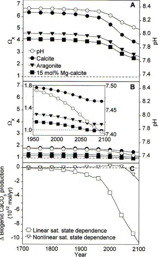
Acknowledgements

        I would like to thank my thesis advisors: Fred T. Mackenzie and Jane E.

Schoonmaker for their unconditional support and infinite patience. Needless to say my

graduation was only made possible by their willingness to go above and beyond for

their students. The completion of this thesis could never have been done without the

assistance of Andreas Andersson to whom I will be eternally grateful. I am extremely

fortunate to have met, and worked with such a true advocate of science. One could only

hope to gain the knowledge and fortitude Andreas reflects in his work.

        I would also like to thank Rene Tada and Kathy Kozuma for their guidance

while I enjoyed my stay in the GES program. Their supervision created a sense of home

in the department.

        Professors, colleagues, and peers that deserve mention for making life in the

GES program interesting, fun, rewarding, and memorable are Eric De Carlo, Michael

Guidry, Laura Degelleke, Christopher Colgrove, Rachel Solomon, Whitney Hassett,

and Megan O’Brian. Each individual mentioned has carved a lasting memory in my

life.

        Finally I would like to thank my family: Tommy Tan, Margaret Tan, Bernice

Tan, Melissa Tan, Linda Cua, Adam Cua, Kathy Cua, Jackie Cua, and Sasha Cua for

supporting my education and providing me a home filled with an atmosphere of love.

No son, brother, nephew, or cousin could ever ask for more.

                                          iii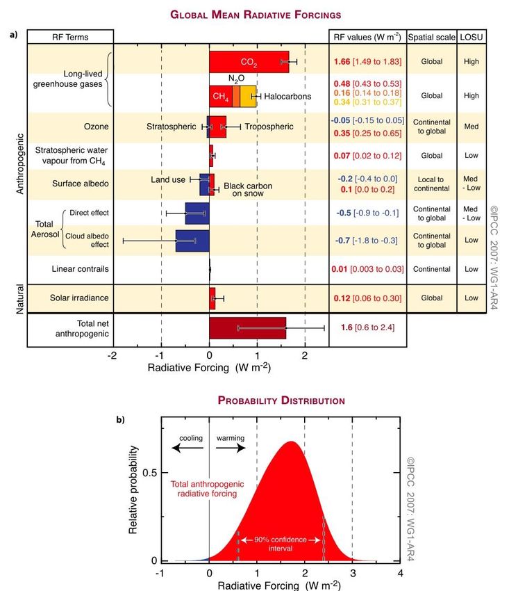
Abstract

       Ocean acidification is the lowering of seawater pH due to increased pCO2 levels

in the atmosphere brought about by human activities of fossil fuel burning and

deforestation. As of 2005 atmospheric pCO2 levels had reached 380 ppm (IPCC, 2007),

the highest level for the last 640,000 years (Petit et al.,1999; Barnola et al.,2003,

Siegenthaler et al., 2005, IPCC, 2007). The increase in pCO2 in the atmosphere is an

immediate concern because of its direct relationship with ocean chemistry. The change

in ocean chemistry due to the addition of CO2 lowers both the pH and saturation state

of seawater with respect to different CaCO3 minerals (Andersson et al., 2003, Morse et

al., 2006). Calcification rates decrease as the saturation state of seawater with respect to

CaCO3 decreases, hence producing weaker skeletons for calcareous organisms. The

weaker coralline structures lead to greater vulnerability to physical and biological

erosion.

       A diurnal study of the effects of increased pCO2 levels in the atmosphere on

calcification rates of corals was done using a flow through mesocosm in which the

coral Montipora capitata was grown. The experiment quantitatively compared the

calcification rates of corals in tanks with an elevated CO2 level of 700 ppm (projected

atmospheric CO2 level by the year 2100) to those of tanks with ambient CO2 levels

(380 ppm). Net ecosystem calcification (NEC) rates were calculated using total

alkalinity (TA) and pH measurements of water flowing in and out of the tanks. The

results of this experiment showed that an elevated CO2 level of ~700 ppm induced a

significant reduction in net calcification rates compared to NEC in the tanks with

                                             iv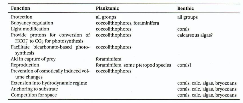
ambient CO2 levels. The calculations of NEC showed average net dissolution rates over

a diurnal cycle for tanks with elevated CO2 levels.

                                            v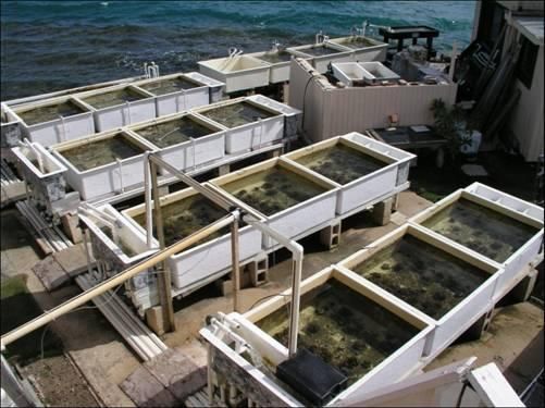
Table of Contents

Acknowledgements ………………………………………………………….......                              iii
Abstract ………………………………………………………………………….                                       iv
List of Table and Figures ……………………………………………………......                        vii
Chapter 1 – Introduction ………………………………………………………...                             1
          1.1 – Global Warming ………………………………………………...                          1
          1.2 – Ocean Acidification ……………………………………………..                       8
          1.3 – Carbonate Chemistry of Seawater ………………………………                10
          1.4 – CO2 Flux Determinants …………………………………………                      12
                  1.4.1 – CO2 Physical Response ………………………………                12
                  1.4.2 – Calcification and Dissolution ………………………...        12
                  1.4.3 – Photosynthesis and Respiration ………………………          14
          1.5 – Objectives of this Study    ……………………………………….                15
Chapter 2 – Experimental Setup and Analytical Methodology …………………           17
          2.1 – Experimental Setup ……………………………………………...                     17
          2.2 – Experimental Tank Measurements ………………………………                 19
          2.3 – Laboratory Analysis …………………………………………….                      20
                  2.3.1 – DIC ……………………………………………………                          20
                  2.3.2 – Total Alkalinity ……………………………………….                 20
                  2.3.3 – Carbonate Species Calculation ……………………….          21
          2.4 – Nature of Samples ……………………………………………….                       21
Chapter 3 – Results ………………………………………………………………                                22
Chapter 4 – Calculations and Discussion of Results ………………………….....          27
          4.1 – pH-TA vs. pH-O2 Method (pH-TA Method Validity) …………..       27
          4.2 – Calculation of Net Ecosystem Calcification Rates ……………...   30
          4.3 – Discussion of Results …………………………………………….                    32
Chapter 5 - Conclusions …………………………………………………………                              36
Appendix A: SRES ………………………………………………………………                                   39
Appendix B: Data: Measurements from Ocean Acidification Experiment ……...    40
Appendix C: Calculations for NEC ………………………………………………                         42
References ………………………………………………………………………...                                   44

                                      vi
List of Table and Figures
Table Page
1 Proposed functions of calcification by different organisms……….………….13
Figures Page
1 Measured and past prediction of global and continental
temperature change…………………………..……………………….….……..2
2 Monthly mean pCO2 levels measured at the Mauna Loa Observatory…..…….3
3 Trends in atmospheric CO2, CH4, and D from 640 Kya to present
from the Vostok ice core……..........………………………………………...…4
4 Historical and projected global warming from 1900 to 2100………………….5
5 Correlation between sunspot cycle lengths and the mean northern hemisphere
temperature record between 1861 to 1989…………………………….……….6
6 Global mean radiative forcing summary…………………………..…………...7
7 Historical and projected saturation state of seawater with respect to
different carbonate minerals……………………………………………………9
8 Aerial photograph of the University of Hawaii Institute of Marine Biology,
Moku o Lo’e, Oahu, Hawaii……………………………………………..........18
9 Control and experimental tanks used in calcification experiment…….…...….19
10 pH, DO, and temperature of the system throughout the 24-hour
ocean acidification experiment…………………………………………….….23
11 Total alkalinity of the system during the 24-hour ocean acidification
experiment………………………………………………………………….....24
12 HCO3-, CO32-, CO2, and total carbon of the system throughout the
24-hour ocean acidification experiment………………………………...….....25
13 Aragonite and calcite saturation states throughout the 24-hour
ocean acidification experiment……………………………………………..…26
14 Total alkalinity box model of the ocean acidification experiment……………30
vii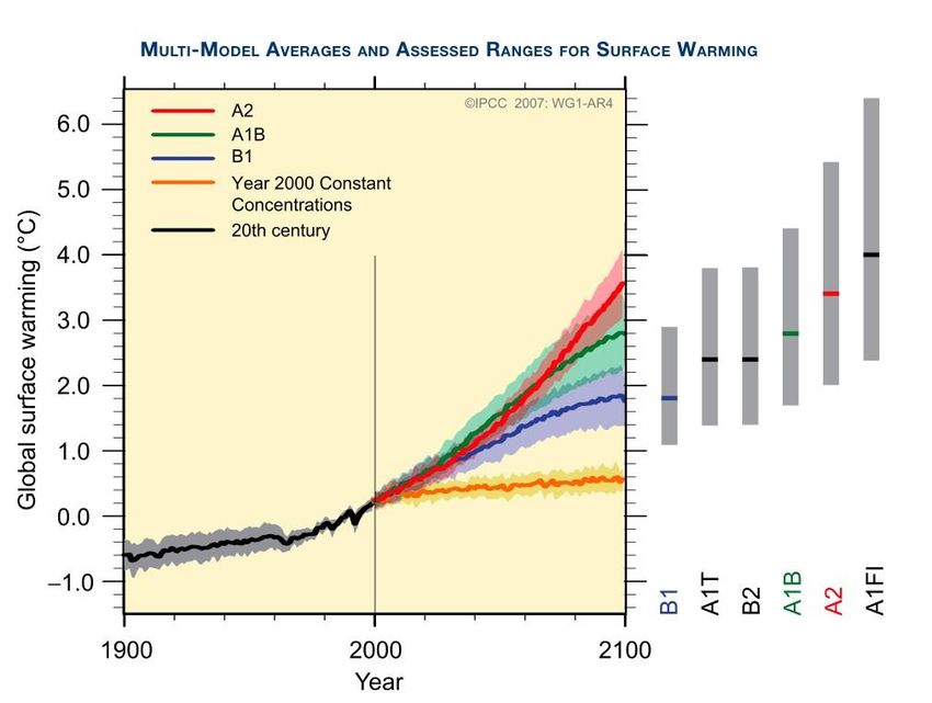
15   Net ecosystem calcification rate throughout the 24-hour ocean
     acidification experiment………………………………………………………33

16   Average net ecosystem calcification rate throughout the 24-hour ocean
     acidification experiment………………………………………………………34

                                   viii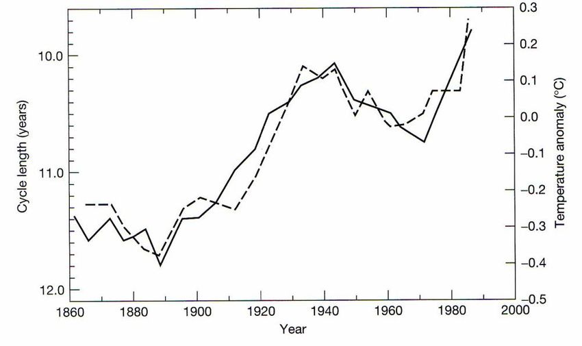
Chapter 1 – Introduction
1.1 – Global Warming
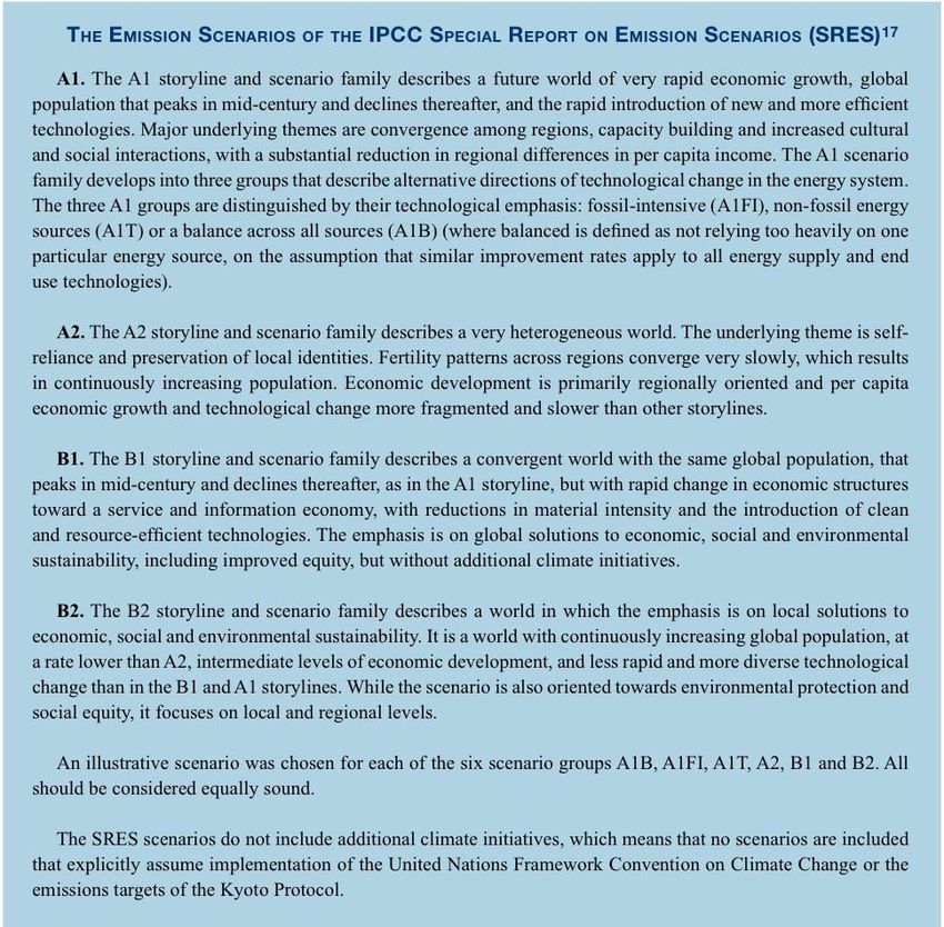
Global warming today is a real concern with real consequences. Figure 1 shows
how global and continental temperatures changed from 1906 to 2005. The figure
compares actual global and continental temperature change to model predictions with
natural and anthropogenic forcings. This figure shows how the change in global
temperature is very close to model predictions that account for anthropogenic forcing.
Anthropogenic forcing in the model is mostly driven by the increase in atmospheric CO2
from fossil fuel burning (Solomon, 2007). CO2 is a major gas of concern for global
warming and should closely be monitored.
As of 2005 atmospheric pCO2 concentrations were at 380 ppmv (IPCC, 2007).
Figure 2 shows the steady increase of pCO2 in the atmosphere from 1958 to present. The
annual CO2 concentration growth rate from 1995 to 2005 was 1.9 ppmv, which is
considerably higher than the average growth rate from 1960 to 2005 of 1.4 ppmv per year
(IPCC, 2007). Houghton (2001) showed that atmospheric pCO2 levels could reach 970
ppmv by the end of the 21st century depending on factors like population growth,
economic growth, technological development, and environmental protection. Models
show that if atmospheric pCO2 stabilized at 750 ppmv in the year 2100, it would still take
more than a thousand years for temperature and sea levels to return to preindustrial values
(Solomon, 2007).
1
Figure 1. Measured and past prediction of global and continental temperature change.
The solid black line is the measured global mean temperature while the thick colored
lines represent model predictions done with different assumptions. The blue line
represents the modeled temperature change not accounting for anthropogenic forcings,
while the pink line represents the modeled results for global and continental
temperature change taking anthropogenic forcings into account (IPCC, 2007).

        According to the analysis of the trapped gas bubbles in Antarctic ice cores

(Figure 3), present values of pCO2 are the highest concentrations observed in 640,000

years (Petit et al.,1999; Barnola et al., 2003; Siegenthaler et al. STET 2005; IPCC, 2007).

This is alarming because the Special Report on Emission Scenarios (SRES) models from

                                            2
the IPCC with different degrees of conservatism all show a distinct increasing trend in
global surface temperature likely driven by CO2 from anthropogenic sources (Figure 4).
Figure 2. Monthly mean pCO2 levels measured at the Mauna Loa
Observatory, Hawaii from 1958 to present. Dr. Pieter Tans, NOAA/ESRL
(www.esrl.noaa.gov/gmd/cgg/trends).
The model projections show that if CO2 emissions were held at year 2000 values,
a temperature increase of 0.1 C per year would be expected; however, if CO2 emissions
increased to IPCC SRES values, an increase of 0.2 C per year would be expected (IPCC,
2007). According to Houghton et al (2001), a 1.4 to 5.8 C in temperature is expected by
the end of the 21st century.
3Figure 3. Trends in atmospheric CO2, CH4, and D from 640 Kya to present from
the Antarctic ice cores. The figure shows the correlation between CO2 and
temperature (D). The record indicates that during this time period CO2 values
never exceeded the present value. (www.realclimate.org)
CO2 levels in the atmosphere have a very strong correlation with temperature;
however, it is still not certain that the increased pCO2 in the atmosphere is the main cause
of the warming of the earth. According to the ice core record, the temperature increase of
the earth has a lag with relation to the pCO2 increase in the atmosphere (Petit et al.,
1999). There is growing evidence that celestial processes (Figure 5) such as solar and
cosmic ray activity also may play a role in regulating the earth’s temperature (Friis-
Christensen and Lassen, 1991; Svensmark 1998). Continuous monitoring of total solar
irradiance now covers the last 28 years (Solomon, 2007). The data show a well
established 11-year cycle in irradiance that varies by 0.08% from solar cycle minima to
maxima, with no significant long-term trend (Solomon, 2007). The primary known cause
of contemporary irradiance variability is the presence of sunspots (compact, dark features
4where radiation is locally depleted) and faculae (extended bright features where radiation
is locally enhanced) (Solomon, 2007). Estimated direct radiative forcing due to changes
in solar output since 1750 is +0.12 [+0.06 to +0.03] W/m2, far less than the radiative
forcing of CO2 in the atmosphere (>1.5 W/m2).
Figure 4. Historical and projected global warming from 1900 to 2100. The solid black line
represents a multi-model global average for surface warming prior to the year 2000. A2,
A1B, and B1 are continuations of 20th century simulations (SRES). The orange line
represents global surface warming if emissions were kept at year 2000 values. The grey
bars on the right indicate the best estimate (solid line within each bar) and the likely range
assessed for the six SRES marker scenarios (IPCC, 2007).
5Figure 5. Correlation between sunspot cycle lengths (solid line) and the mean
northern hemisphere temperature record between 1861 to 1989 (Friis-
Christensen and Lassen, 1991; Svensmark and Solanki, 2002).
Figure 6 summarizes the different radiative forcings (RF) that affect the earth’s
mean global temperature. Factors that affect RF are: long lived greenhouse gasses, ozone,
water vapor from CH4, surface albedo, aerosols, and solar irradiance (Solomon, 2007).
By accounting for these RF factors, it can clearly be seen that anthropogenic radiative
forcing outweighs that of the natural RF. The greatest contributor for RF is CO2, which is
mostly of anthropogenic origin. The increasing concentrations of CO2 in the atmosphere
lead to global warming and ocean acidification.
6Figure 6. Global mean radiative forcing (RF) summary. (a) Shows all the factors that
contribute to global mean RF. Factors include both natural and anthropogenic forcings.
The forcings labeled red contribute to global warming, while forcings labeled blue oppose
global warming. (b) Probability distribution of the global mean combined RF from all
anthropogenic agents shown in (a). Distribution is calculated by combining the best
estimates and uncertainties of each component (Solomon, 2007).
71.2 – Ocean Acidification
The ocean is the largest labile reservoir for carbon on decadal to millennial
timescales. The ocean acts as a variable sink for atmospheric pCO2 and other climate-
relevant trace gasses (Siegenthaler and Sarmiento, 1993). pCO2 in the atmosphere would
be much higher if not for the ocean acting as a carbon sink. At present, roughly 50% of
the anthropogenic CO2 in the atmosphere is transported to the ocean by physical
processes (Sabine et al., 2004, Morse et al., 2006). Estimates of the ocean CO2 uptake for
the last 20 years amount to 1/3 of the CO2 released from fossil fuel burning alone
(Prentice et al., 2001). Models suggest that on millennial timescales the ocean will be the
ultimate sink for about 90% of the anthropogenic carbon released to the atmosphere
(Archer et al., 1998). However, the ocean cannot be regarded as an unlimited sink for
anthropogenic carbon. Under future greenhouse warming climate scenarios, the ocean’s
physical uptake capacity of anthropogenic carbon is expected to decline. This decline is
due to surface warming, increased vertical stratification, and possibly a slowed
thermohaline circulation (Sarmiento et al., 1998).
The increase in pCO2 in the atmosphere is of great concern because of its direct
relationship with ocean chemistry. As pCO2 in the atmosphere increases from fossil fuel
emissions and other anthropogenic sources of CO2, the ocean consequently takes up more
CO2, hence changing its chemistry with poorly known consequences for marine life
(Kleypas et al., 2006, Morse et al., 2006). The change in water chemistry lowers the pH
and saturation state of seawater with respect to different CaCO3 minerals (Figure 7)
(Andersson et al., 2003, Morse et al., 2006).
8Figure 7. Historical and projected saturation state of seawater with respect to
different carbonate minerals in (a) surface water and (b) pore water. (c)
Modeled changes in saturation state result in declines in biogenic CaCO3
production. (Andersson et al., 2003)
Calcification rates decrease as seawater carbonate saturation states decrease
(Figure 7c). Lowered calcification rates may cause the production of weaker calcareous
skeletons and greater vulnerability to physical erosion for calcifying organisms leading to
unhealthy and unstable reefs. In addition to increased susceptibility to physical erosion,
as the coralline structure gets weaker, macrobioerosion (mollusks and sponges) and
9microbioerosion (fungi and microalgae) may play an even more pronounced role in the
ecosystem (Kleypas et al., 2006).
Alternatively, it has been suggested that projected changes in seawater chemistry
will not significantly affect marine calcifiers. This is due to the argument that any
changes in saturation state and pH will be restored by dissolution of metastable carbonate
minerals (Halley and Yates, 2000; Barnes and Cuff, 2000). However, according to
numerical models done by Andersson et al. (2003), reactions in marine porewaters are
not able to buffer the entire water column. Andersson’s model suggests dissolution of
metastable carbonate phases within the porewater-sediment system will not generate
enough total alkalinity to buffer the pH or carbonate saturation state of the entire water
column.
1.3 – Carbonate Chemistry of Seawater
The dissolved inorganic carbon (DIC) chemistry in seawater is complex in that
CO2 reacts to produce carbonic acid and other dissolved inorganic carbon species. The
distribution of inorganic carbon species in a system is a function of temperature, salinity,
and pressure. Increases in atmospheric pCO2 will lead to more CO2 invasion to the ocean,
hence increasing the DIC in the mixed layer of the ocean. Consequently, CO 32-
concentrations will decrease, lowering the saturation state of seawater with respect to
carbonate minerals (Andersson et al., 2003). The following equations represent the DIC
system reactions (Morse and Mackenzie, 1990):
CO2 (g) CO2 (aq) (1)
CO2 (aq) + H2O H2CO30 (2)
10H2CO30 HCO3- + H+ (3)
HCO3- CO32- + H+ (4)
_________________________________
CO2 (g) + H2O + CO32- 2HCO3- (5)
The ocean contains 50 times more inorganic carbon than the atmosphere. There
are 3 pools of oceanic DIC: HCO3- (90%), CO32- (9%), and dissolved CO2 (1%) (Gattuso
et al., 1999). CO2 in surface waters is close to equilibrium with the atmosphere.
Calcification is coupled with the DIC system. The carbon atom that is incorporated in the
production of CaCO3 is from HCO3-.
Ca2+ + HCO3- CaCO3 + H+ (6)
H+ ions are released in the process of calcification hence making seawater more acidic.
The additional acid pushes HCO3- across into the oceanic CO2 pool.
Ca2+ + 2HCO3- CaCO3 + CO2 + H2O (7)
Physical equilibrium between the oceanic and atmospheric CO2 pools determines whether
the flux of CO2 is to or from the ocean (Gattuso et al., 1999). The DIC system is
important in seawater chemistry in that it functions as a buffer for seawater pH on time
scales of up to several thousand years (Pilson, 1998).
The removal of DIC, redistribution of the dissolved carbonate species, and
changes in the relative concentration of CO2 in solution are controlled significantly by the
precipitation of CaCO3 mineral phases and biological production of organic matter
(Lerman and Mackenzie, 2005). The rates at which these factors change affect the CO2
flux across the air-sea interface. According to the stoichiometry of Equation 7 for
calcification, precipitation of calcium carbonate will raise the pCO2 of the system while
11dissolution lowers it. This ultimately may lead to changes in the CO2 concentrations in
other reservoirs (Lerman and Mackenzie, 2005). Over glacial-interglacial timescales,
preservation and dissolution of CaCO3 in ocean sediments act to maintain a nearly
constant ocean alkalinity that provides a significant negative feedback on changes in
atmospheric pCO2 (Archer, 1996).
1.4 – CO2 Flux Determinants
1.4.1 – CO2 Physical Response
Shallow water ocean environments, i.e. bays, estuaries, lagoons, banks, and
continental shelves, constitute ~7% of global ocean surface area, but are the source of 10-
30% of the world’s marine primary production (Gattuso et al., 1998). These regions are
important with respect to the carbon flux because 85% of the organic carbon and 45% of
the inorganic carbon in the ocean are buried in shallow water ocean sediment
environments. According to Andersson and Mackenzie (2004), the net flux of CO2
between the ocean and the atmosphere is dependent in part on the partial pressure
gradient between the two. Calcification, dissolution, photosynthesis, and respiration
influence the partial pressure gradiant and thus also play major roles in determining the
net flux of CO2.
1.4.2 – Calcification and Dissolution
Calcification evolved sometime during the Cambrian period, coincident perhaps
with a sudden rise in Ca2+ (e.g. Kleypas et al., 2006). Since high concentrations of Ca2+
are toxic to cellular processes, it has been proposed that calcification may have been the
detoxification mechanism at the time (Brennan et al., 2004). Organisms since then have
12harnessed this evolutionary process to produce CaCO3 shells and skeletons for protection
and other functions (Table 1). Predictions of how reduced calcification rates will affect
different organisms are based on the assumption that calcification serves multiple
functions that benefit different species (Kleypas et al., 2006).
Table 1. Proposed functions of calcification by different organisms (Kleypas et al.,
2006)
Calcification is a CO2-releasing process that can make seawater initially in
equilibrium with the atmosphere degas against the initial pCO2 gradient (Ware et al.,
1992). In this respect, most coral reefs are actually CO2 sources and not CO2 sinks (Ware
et al., 1992). Coral reef building requires that calcification exceeds dissolution so that any
growing coral reef system is a net source of CO2, hence contributing to greenhouse
gasses in the atmosphere. This is a positive feedback, until a certain threshold, for coral
growth because according to Mackenzie and Agegian (1989), the rate of calcification of
coralline algae and corals exhibits a strong positive correlation to saturation state and a
negative parabolic dependence on temperature, a statement documented in numerous
other experiments.
13The precipitation of CaCO3 minerals from supersaturated water is accompanied
by a decrease in total alkalinity and an increase in dissolved CO 2 and H+ ion
concentration, which results in a lowering of the seawater pH (Lerman and Mackenzie,
2005). Equation 8 shows the stoichiometry of calcification. The forward reaction denotes
precipitation while the backward reaction denotes dissolution.
Ca2+ + 2HCO3- CaCO3 + H2O + CO2 (8)
The equation shows the relationship between calcification, CO2 production, and
total alkalinity. Calcification removes two moles of carbon from solution and produces
one mole of CO2, while dissolution consumes CO2 and produces HCO3-. Two equivalents
of TA are produced for every mole of CaCO3 dissolved.
1.4.3 – Photosynthesis and Respiration
Primary production consumes CO2 and respiration of organic matter produces
CO2. Equation 9 shows the stoichiometry of photosynthesis and respiration. The forward
reaction denotes gross primary production while the backward reaction denotes
autorespiration.
CO2 + H2O CH2O + O2 (9)
The main site for marine calcification is the euphotic zone (upper ~50 m of ocean water)
where calcifying organisms (phytoplankton, zooplankton, zoobenthos) thrive (Lerman
and Mackenzie, 2005). In euphotic zones where the gross primary production greatly
exceeds autorespiration, the removal of CO2 may essentially compete with carbonate
precipitation that generates CO2 that can be emitted to the atmosphere (Equation 8)
(Lerman and Mackenzie, 2005). Some of the calcium carbonate produced in surface
14coastal and open ocean water dissolves in the water column and in sediments. These
dissolution reactions are driven by CO2 produced during remineralization of sinking
organic matter deposited in sediments that produces CO2 (Emerson and Bender, 1981).
This process results in the return of carbon taken up in calcification and organic matter
production back to ocean water as alkalinity and DIC, respectively.
The dissolution of CaCO3 in reef environments is expected to increase in response
to ocean acidification. Net carbonate dissolution is observed in many reef environments
at night (Kleypas et al., 2006). This occurs when respiration greatly increases and
elevates the local pCO2 of the water column. Dissolution is likely to be occurring all the
time in the sediments and carbonate framework of reefs; however, it is only evident at
night when it is not masked by a higher rate of carbonate precipitation (Kleypas et al.,
2006). In a strongly autotrophic ecosystem, CO2 production by calcification may be
counteracted by organic productivity through uptake of the generated CO2, resulting in
lower CO2 transfer rates from the ocean to the atmosphere, or ultimately a reversal
(Lerman and Mackenzie, 2005).
1.5 – Objectives of this Study
It is anticipated that increased acidification of the oceans from uptake of CO2 will
result in decreased calcification rates of marine organisms (e.g., Kleypas et al., 2006).
The extent of reduction of calcification rates as a function of pCO2, however, is not well
characterized. In addition, although some calcifying organisms are known to undergo
dissolution at night, they are net calcifiers on a diurnal basis under current oceanic
saturation states. It is not known how much CO2 is required to force a calcifying system
to a state of net dissolution on a diurnal basis. The objective of this study was to
15investigate the effects of ocean acidification on coral calcification rates. Specifically,
experiments were designed to quantify the calcification rates over a 24-hour cycle of
corals exposed to two different levels of pCO2.
A mesocosm experiment using two sets of tanks with different pCO2 levels was
conducted to compare the net ecosystem calcification rate of a system with a raised pCO2
level of ~700 ppm (experimental tank) with that of a system with an ambient pCO2 level
of 380 ppm (control tank). My hypothesis is that the difference in pCO2 levels of the
control and experimental tanks will be significant enough to cause a distinct decline in
net ecosystem calcification rates for the experimental tank.
16Chapter 2 – Experimental Setup and Analytical Methodology
2.1 – Experimental Setup
A diurnal study of the effects of increased pCO2 levels in the atmosphere on
calcification rates of coral was done at the Hawaii Institute of Marine Biology in Moku O
Lo’e (Coconut Island), Southern Kaneohe Bay, Hawaii (Figure 8). Six fiberglass tanks of
0.5 m3 (1 x 1 x 0.5 m) were flushed with running seawater (~8 L min-1) directly pumped
from the edge of the coral reef (Figure 9). The experimental design involved growth of a
single species of coral (Montipora capitata) in a series of flow-through mesocosms.
Inflow waters in half of the mesocosms were manipulated to increase artificially pCO2
levels. The carbonate chemistry of the inflow and mesocosm tank waters was monitored,
and the differences were used to calculate rates of calcification in each of the mesocosms.
The experiment started at 12:00 noon on June 22, 2006 and ended at 12:00 noon the next
day.
The residence time of the water in the tanks was approximately 1 hour. All of the
tanks had corals of the same species and comparable sizes (see section 2.4). Three tanks
were used as experimental tanks for manipulation of seawater pCO2. Concentrated
hydrochloric acid (HCl) mixed with fresh water to a 10% solution was added to the
seawater flowing into the experimental tanks. The acid was added using a 205CA Watson
Marlow multichannel peristaltic pump at a rate of 1.3 ml min-1 through 2.05 mm tubing.
HCl added to the system shifted the distribution of dissolved carbonate species,
increasing the pCO2. The resulting seawater was equivalent to that in equilibrium with an
atmosphere having a pCO2 of 745 + 130 ppmv. This CO2 level is slightly lower than the
17expected pCO2 levels in the end of the 21st century following a business as usual (BAU)
scenario (Houghton et al., 1996, 2001). In the remaining three control tanks, fresh water
was added at the same rate as HCl was added to the experimental tanks. Measurements of
temperature, pH, and dissolved oxygen (DO) in all six tanks were taken in two hour
increments, while samples for salinity, total alkalinity (TA) and dissolved organic carbon
(DIC) were taken every four hours. The experimental setup was the same as that used by
Kuffner et al. (in press) and Rodgers et al. (in press). The data from this experiment are
shared between all authors.
Figure 8. Aerial photograph of the University of Hawaii Institute of Marine Biology,
Moku o Lo’e, Oahu, Hawaii. (Photograph taken from Coconut Island Website -
http://www.hawaii.edu/HIMB/)
18Figure 9. Control and experimental tanks used in calcification experiment under
present and elevated CO2 conditions located at the University of Hawaii Institute of
Marine Biology, Moku o Lo’e, Oahu, Hawaii. (Photograph courtesy of Ku’ulei
Rodgers of Hawaii Institute of Marine Biology)
2.2 – Experimental Tank Measurements
Temperature and salinity were measured in each tank using a YSI 30 salinity/
conductivity/temperature meter with accuracies of +0.1 °C and +0.1 ppt, respectively.
Dissolved oxygen was measured using a YSI 95 Dissolved Oxygen Microelectrode Array
Model with an accuracy of +0.2 mg L-1. The pH of each tank was measured using a fully
enclosed Oakton Ag/AgCl combination electrode attached to an Accumet AP72 handheld
pH/mV/temperature meter with an accuracy of +0.01 pH units. The pH electrode was
calibrated using 4.00 and 7.00 NBS buffer solutions from Fisher Scientific (+ 0.01 pH
units @ 25 C). Water samples for total alkalinity were collected of surface seawater in
each tank using 200 mL Kimax brand glass sample bottles and were poisoned with a
saturated solution of mercuric chloride (HgCl2). 100 L of HgCl2 solution were added to
each sample. Each bottleneck was taped with Teflon tape prior to sampling to assure a
19tight seal and prevent atmospheric equilibration of gasses. Dissolved inorganic carbon
samples were collected in a similar manner to alkalinity (Kuffner et al., in press).
2.3 – Laboratory Analyses
2.3.1 – DIC
Seawater samples collected for DIC were analyzed using a Li-Cor 6262 NDIR as
a detector. Unfortunately the DIC results could not be used in the interpretations
described in this paper. This was due to the fact that the sample bottles were not stored
properly and CO2 was exchanged with the atmosphere.
2.3.2 – Total Alkalinity
Collected seawater samples for total alkalinity were titrated using the
potentiometric acid titration (DOE, 1994). The system was modified by Dr. Rolf
Arvidson of Rice University, Houston, Texas during his affiliation with the University of
Hawaii. The alkalinity driver routine (GranPlot) and the fitting routine (GranFit) were
modified to be able to adjust the “Gran boundary”, “Gran pts”, and “Gran pts to fit” to
obtain a precision of 0.15%. The Gran pts and boundaries are internal parameters of the
program to adjust for precision and accuracy of the titration. The Accumet calomel
combo electrode was attached to an Orion expandable ion analyzer EA920. The
Brinkmann Metrohm Dosimat was used to dispense 0.1 M HCl for titrations. Both
apparatuses were remotely controlled by a GranPlot driver. The 0.1 M HCl acid was
standardized against certified reference material (CREM) prepared by Andrew Dickson at
Scripps Institution of Oceanography. CREMs were analyzed after every 7th sample
20determination to ensure accuracy and precision of the titration. Titrations were accurate
and precise to less than 1% error.
2.3.3 – Carbonate Species Calculation
The carbonate species were calculated using the CO2SYS software program
(Lewis and Wallace, 1998). The CO2 system parameters were calculated at in situ
temperature and salinity from total alkalinity and pH employing stoichiometric carbonic
acid system constants calculated on the NBS scale by Peng et al. (1987) based on the
constants defined by Mehrbach et al. (1973).
2.4 – Nature of Samples
The seawater chemistry in both the control and experimental tanks was given four
weeks to stabilize prior to the introduction of coral colonies. Two sets of Montipora
capitata colonies of comparable size (~10 cm diameter) and morphology were collected.
The two colonies were collected at similar depths off Moku O Lo’e Island. One colony
came from the windward flat reef, and the other at the fringing reef south of the island.
Twenty colonies from the two sets were randomly picked and placed in the experimental
and control tanks (Rodgers, in press).
21Chapter 3 – Results
Results of the diurnal experiment as described in Chapter 2 are summarized in the
figures below. Figure 10 shows the pH (Figure 10a), dissolved oxygen (DO) (Figure
10b), and temperature (Figure 10c) of each of the tanks. Symbols in blue represent the
control tanks (8, 10, 12) and symbols in red represent the experimental tanks (7, 9, 11).
The dashed line represents the input characteristics of the seawater from Kaneohe Bay,
and reflects the natural external variance of the parameters being measured.
The pH of the system falls at night owing to the lack of photosynthesis and
reduced calcification. As photosynthesis decreases and respiration increases at night, the
amount of CO2 in solution increases, hence lowering the pH of the system. Equation 6
(calcification equation) shows that for every mole of CaCO3 produced, 1 mole of H+ is
also produced, hence further lowering the pH of the system. However, the reduced
calcification at night implies less protons produced by this reaction. In addition,
photosynthesis releases O2 during the day, and respiration uses up O2 at night. As can be
seen in Figure 10, photosynthesis plays an important role in the system. As would be
predicted, the temperature of the system is the lowest before daybreak at about 6 am and
the highest past noon at about 2 pm. This is because water has a high specific heat and
therefore heats up slowly, and conversely releases heat slowly as well.
22(a) (b)
8.3 9.5
8.2 9
8.1
Dissolved oxygen (mg/L)
8.5
8 7 7
8 8 8
7.9 9
pH-NBS
9
10 7.5 10
7.8 11 11
12 7 12
7.7 in in
7.6 6.5
7.5 6
7.4 5.5
12:00 16:00 20:00 0:00 4:00 8:00 12:00 12:00 16:00 20:00 0:00 4:00 8:00 12:00
Time Time
28.5
28.25
28
27.75
27.5
7
27.25 8
27 9
10
26.75
11
26.5 12
26.25 in
T
26
25.75
25.5
25.25
12:00 16:00 20:00 0:00 4:00 8:00 12:00
Time
(c)
Figure 10. pH, DO, and temperature of the system throughout the 24-hour ocean
acidification experiment. (a) The pH of the system decreases at night when
respiration exceeds photosynthesis and releases more CO2 to the system. (b) DO
decreases at night when respiration exceeds photosynthesis and uses up the available
DO in the system. (c) Temperature of the system fluctuates with respect to the
temperature variance of night and day. The dashed line represents the input solution,
which is seawater pumped directly from Kaneohe bay.
The total alkalinity (TA) of the system behaves as predicted. As can be seen in
Figure 11, TA is lowest during the day. This is due to the calcification process using up
free HCO3- in the system (Equation 6). The reduction of free HCO3- in the system causes
TA to decrease.
232225
2200
2175
2150
2125 7
TA (micromoles/kg)
8
2100 9
2075 10
2050 11
12
2025 in
2000
1975
1950
1925
12:00 16:00 20:00 0:00 4:00 8:00 12:00
Time
Figure 11. Total alkalinity of the system during the 24-hour ocean acidification
experiment. Total alkalinity is controlled by the uptake and release of HCO3- in the
system through calcification. As more calcification occurs, more HCO3- is used.
Calcification is prominent during the day hence the lower TA.
The carbonate system is closely tied to photosynthesis/respiration and
calcification/dissolution processes. Figure 12c shows how CO2 increases at night via
respiration, and decreases during the day via photosynthesis. Through the DIC equations
(Equations 1 to 5), it can be seen that as more CO2 is added to a system, HCO3- (Figure
12a) is produced. CO32- (Figure 12b) decreases at night because H+ ions react with it to
produce more HCO3-. This leads to the fluctuation in the concentration of HCO3- with
respect to time. The graph shows this pattern perfectly. Changes in the total carbon (TC)
of the system (Figure 12d) are also driven by photosynthesis and calcification. At night
when respiration is greater than photosynthesis, CO2 is produced contributing to more TC
in the system. Calcification at night is at a minimum hence less HCO3- in solution
(Equation 8) is taken from the water, further increasing the TC of the system.
241925 250
1900 240
1875 230
220
1850
210
1825 200
1800 190
1775
HCO3 (micromoles/kg)
7 180 7
CO3 (micromoles/kg)
1750 170 8
8
1725 160
9 9
1700 150
10 140 10
1675
11 130 11
1650
12 120 12
1625
110
1600 100
1575 90
1550 80
1525 70
1500 60
1475 50
12:00 16:00 20:00 0:00 4:00 8:00 12:00 12:00 16:00 20:00 0:00 4:00 8:00 12:00
Time Time
(a) (b)
1900
1800 2065
1700
2045
2025
1600
2005
1500
1985
1400
pCO2 (micromoles/kg)
1965 7
1300 7 1945 8
TC (micromoles/kg)
1200 8 1925
1100 9 1905 9
1000 10 1885 10
900 11 1865 11
800 12 1845 12
700 1825
600 1805
500 1785
400 1765
300 1745
200
1725
12:00 16:00 20:00 0:00 4:00 8:00 12:00 12:00 16:00 20:00 0:00 4:00 8:00 12:00
Time Time
(c) (d)
Figure 12. HCO3-, CO32-, CO2, and total carbon of the system throughout the 24-hour
ocean acidification experiment. (a) HCO3- increases at night when more is produced via
the increase of CO2 in the system from respiration. (b) CO32- decreases at night when
CO2 increases producing more H2CO3, which dissociates to produce HCO3-. (c) CO2
rises at night due to the increase of respiration. (d) The total carbon of the system is
dependent on photosynthesis and respiration, and calcification and dissolution which
dictate the addition and removal of CO2, driving the DIC in either direction.
The saturation state of seawater with respect to (a) aragonite and (b) calcite
(Figure 13) is defined here as the product of the concentrations of dissolved Ca2+ and
carbonate ions divided by their product at equilibrium.
([Ca2+] x [CO32-]) / KCaCO3 = (10)
When = 1, the solution is saturated with respect to CaCO3. When exceeds 1 then the
solution is supersaturated. less than 1 denotes undersaturation of seawater with respect
25to CaCO3. As CO2 is added to the system, more H+ ions are released. The excess H+ ions
combine with CO32- hence producing more HCO3-. Figure 13 shows how the saturation
states for both aragonite and calcite decrease at night when excess CO2 is added to the
system through respiration, and increase during the day when photosynthesis exceeds
respiration hence reducing CO2. As seen in Figure 13, the increase in pCO2 in the
experimental tanks (red symbols) results in lower saturation states with respect to both
calcite and aragonite relative to conditions in the control tanks (blue).
4.25 6.25
4 6
5.75
3.75 5.5
3.5 5.25
5
Aragonite Saturation State
3.25 4.75
Calcite Saturation State
3 7 4.5 7
8 4.25 8
2.75 4
9 9
2.5 3.75
10 3.5 10
2.25 11 11
3.25
2 12 3 12
1.75 2.75
2.5
1.5 2.25
1.25 2
1.75
1 1.5
0.75 1.25
12:00 16:00 20:00 0:00 4:00 8:00 12:00 12:00 16:00 20:00 0:00 4:00 8:00 12:00
Time Time
(a) (b)
Figure 13. Aragonite and calcite saturation states throughout the 24-hour ocean
acidification experiment. (a) Aragonite and (b) calcite saturation states decrease at night
when CO2 from respiration increases. The increase in CO2 releases H+ ions, hence
lowering pH. The H+ ions react with CO32- hence lowering the saturation state.
26CHAPTER 4 – Calculations and Discussion of Results
4.1 – pH-TA vs. pH-O2 method (pH-TA Method Validity)
There are two tested methods to measure community metabolism as described by
Gatusso et al. (1999), the pH-TA method and the pH-O2 method. The pH-TA method
deals with values of pH in a given system measured continuously and the total alkalinity,
which is measured at discrete time intervals. The fact that TA cannot be measured
instantaneously gives rise to criticism of the use of this method. The pH-TA method is
based on measurements of pH and total alkalinity upstream (input) and downstream
(output) of a community. The measurements are then used to calculate the difference
between the upstream and downstream concentrations of dissolved inorganic carbon
(DIC) using stoichiometric equations that describe the seawater carbonate system.
Equation 11 is used to calculate the rate of calcification using TA and calcification
relationships.
Ca2+ + 2HCO3- CaCO3 + CO2 + H2O (TA=-2eq) (11)
However, a 1:1 molar relationship between CO2 and CaCO3 only holds true for
freshwater. The ratio is lower for seawater because of its buffering capacity
(Frankignoulle, 1994).
A major assumption to keep in mind in the pH-TA method is the assumption that
there is no process other than calcification that significantly affects TA, and that the
removal and addition of CO2 from photosynthesis and respiration do not play a role in the
TA calculations. However, photosynthesis and respiration are coupled with assimilation
and dissimilation of NH4+, NO3-, and HPO42-, which liberate OH- or H+ (or uptake H+ or
27OH-) as shown in equations 12a and 12b. The forward reactions for Equations 12a and
12b represent photosynthesis as written and respiration is in the reverse direction.
106CO2 +16NH4+ + HPO42- + 106H2O C106H263O110N16P + 106O2 + 14H+ (12a)
106CO2 +16NO3- + HPO42- + 122H2O + 18H+ C106H263O110N16P + 138O2 (12b)
Nitrification and sulfate reduction reactions alter the TA of a system more significantly as
shown in equations 13 and 14.
NH4+ + 2O2 NO3- +2H+ + H2O (TA=-2eq) (13)
SO42- + 2H+ H2S + 2O2 (TA=2eq) (14)
However, this does not invalidate the method, because as shown by Kinsey (1978), the
summation of equations 11 to 14 is likely to cause less than a 5% error in the net
calcification rates calculated for specific reefs. A bigger potential problem with the pH-
TA method is that organic acids can significantly contribute to TA in euphotic
environments (Cai and Wang, 1998), but concentrations of organic acids in reef settings
are not overly high. A study by Cai and Wang (1998) shows that the organic acid
alkalinity behaves conservatively in organic rich estuaries in Georgia. This is a
reasonable assumption for ocean water as well because the DOC is comparable, and
ocean water has a much lower concentration of organic acids. Also, because TA
measurements in community metabolism deal with changes in TA over time (not absolute
values), the effects are negligible. Finally, the validity of the TA anomaly technique to
estimate coral calcification has been repeated many times and is well established (Smith
and Kinsey., 1978; Tambutte, E., et al., 1995).
28The pH-O2 method addresses the shortcomings of the pH-TA method wherein
discrete samples are needed to be analyzed for TA. The pH-O2 method was introduced by
Barnes (1983) as a means to calculate continuous calcification rates and not be limited by
discrete time intervals from TA data. The pH-O2 method uses relationships between O2,
DICorg (net community production), and metabolic quotients to estimate net community
production and respiration from changes in the concentration of DO. DICorg is
calculated by subtracting DICcalc (changes in DIC from calcification) from the total
DIC. Metabolic quotients are calculated from net community photosynthesis
(O2/DICorg) and respiration (DICorg/O2). The change in TA and net community
calcification are estimated by using the stoichiometric relationships given in Equation 11.
The pH-O2 method is very attractive because instruments today have very precise
and reliable sensors to monitor pH and DO in the field. However, a major drawback of
the pH-O2 method is that it requires the use of assumed values like O2:CO2 ratios to
calculate the metabolic quotient. The assumptions used to calculate specific metabolic
quotients introduce uncertainty to the calculated metabolic parameters.
This method was not chosen for this experiment because of the uncertainty that
comes with assuming a specific metabolic quotient for a community. Any biochemical
process that yields a ratio of O2:CO2 that is stoichiometrically different from the assumed
metabolic quotient complicates the pH-O2 method. This can be seen from the nitrification
equation where 2 moles of O2 are used per mole of NH4+ nitrified (Equation 13).
294.2 – Calculation of Net Ecosystem Calcification Rates
A simple box model (Figure 14) was created to represent the TA of the flow
through system setup for this experiment. F1 represents the TA input flux of the system
while F2 represents the TA output flux. Calcification and dissolution, are processes that
contribute to the change in TA at discrete times. F1 for the control tanks corresponds to
the flux of total alkalinity associated with the source water from Kaneohe Bay. This TA
fluctuates slightly with time (Figure 11). The total alkalinity flux (F1) for the
experimental tanks is reduced due to the addition of dilute HCl to raise the pCO2 of the
system. Net ecosystem calcification (NEC) calculations are utilized to quantify
calcification rates of both control and experimental tanks.
F1 Total Alkalinity F2
Dissolution Calcification
Figure 14. Total alkalinity box model of the ocean acidification experiment. Total
alkalinity of the system is the algebraic summation of F1, F2, calcification and
dissolution. F1 represents the flux of TA in the input solution. F2 represents the flux of
TA leaving the system. The box model is used to calculate the NEC of both the control
and experimental tanks. Calcification or dissolution can be calculated by subtracting the
sum of F1 and F2 from the total change in alkalinity; a positive value denotes
calcification while a negative value denotes dissolution.
30NEC is used to quantify the difference in calcification rates of the control tanks
with ambient pCO2 levels, as compared to the experimental tanks with elevated pCO2
levels. The NEC is calculated using Equation 15. F1 and F2 are subtracted from the total
change in alkalinity of the system. The result is then divided by two to get the
calcification, or dissolution rate of the system. A positive value for the result means
calcification is occurring while a negative value means there is net dissolution.
NEC (mol/hr) = [dTA/dt (mol/hr)– F2 (mol/hr ) + F1 (mol/hr)] / 2 (15)
dTA/dt represents the change in TA of the system with respect to time. This is calculated
using Equation 16.
dTA/dt (mol/hr)=[TAtime1(mole/Kg)–TAtime2(mole/Kg)]/4 (hrs) x 500 (Kg) (16)
The difference between TAtime1 and TAtime2 is divided by 4 hours to account for TA
measurements that were taken in 4-hour time intervals, and then multiplied by 500 Kg to
account for the mass of the water in the tank. F1 represents the input TA flux of the
system. Equation 17 is used to calculate the F1 for the control tanks.
F1 (mol/hr) =
(flowratetank (Kg/hr)) x [(TAinput(time2) (mol/Kg) + TAinput(time1) (mole/Kg))/2] (17)
F1 is calculated by multiplying the flow rate of the tank by the average TA of the input
tank between time 1 and time 2. The TA input flux has to be corrected for the
experimental tanks wherein dilute acid is added. The F1 for the experimental tank is
represented by equation 18.
31F1 exp (mol/hr) =
(flowratetank (Kg/hr)) x [(TAinput(time2)(mol/Kg) + TAinput(time1)(mol/Kg))/2] – acid
addition (mol/Kg) (18)
The addition of acid (mol/hr) is subtracted from the flow rate of the experimental tank
because it removes TA from the system. The acid addition is represented by Equation 19.
Acid Addition (mol/hr) =
(pump speed (Kg/hr)) x (H+ concentration (mol/kg)) (19)
F2 (mol/hr) is calculated by multiplying the average TA between time 1 and time 2 in
both the control and experimental tanks by the flow rate (mol/hr) . This is represented in
Equation 20.
F2 (mol/hr) =
(flowratetank (Kg/hr)) x [(TAtank(time2)(mol/Kg) + TAtank(time1)(mol/Kg))/2] (20)
The combination of equations 15 to 20 allows for the calculation of the NEC of
the system. Factors in the natural system that were not accounted for in calculating NEC
include gas exchange between the atmosphere and seawater in the tank, and evaporation.
4.3 – Discussion of results
The NEC values are shown in Figure 15. The blue symbols represent the control
tanks (tanks 8, 10, 12), while the red symbols represent the experimental tanks (tanks 7,
9, 11). As expected, calcification rates are noticeably lower for the experimental tanks.
3220000
15000
Net Ecosystem Calcification (micromoles of CaCO3/hr)
10000
5000
8
0 10
12
7
-5000 9
11
-10000
-15000
-20000
-25000
12nn-4pm 4pm-8pm 8pm-12mn 12mn-4am 4am-8am 8am-12nn
time
Figure 15. Net ecosystem calcification (NEC) rates throughout the 24-hour ocean
acidification experiment. All the control tanks (blue) show calcification during the
day, and dissolution at night. This is what is expected in natural systems. Only tank 7
of the experimental tanks shows constant dissolution, however the NEC values of the
experimental tanks are generally lower than those of the control tanks. Tank 8 of the
control tanks reached a dissolution rate similar to the range of experimental tanks
between 8 pm to 12 mn.
Figure 15 shows the NEC results for the ocean acidification experiment. The
control tanks (blue) show calcification during the day, and dissolution at night. This is
what is expected in natural systems because of photosynthesis and respiration. NEC rates
for experimental tanks (red) are interesting in that the trends are the same as those of the
control tanks; however, these tanks display a much lower rate of calcification during the
day, and higher dissolution rates at night. This indicates that although calcification still
occurs at CO2 levels of >700ppmv, dissolution at night exceeds calcification during the
day which means a net dissolution occurs during a 24-hour cycle. Figure 16 shows this
trend more clearly. The average of all control tanks (blue bars) shows calcification
33throughout the day, and dissolution at night when respiration exceeds photosynthesis.
The average of all experimental tanks shows dissolution throughout the day. Although
this scenario is more likely to occur in natural systems slowly, perhaps allowing the
corals to adapt, the significant difference in NEC of the experimental tanks as compared
to the control tanks provides strong evidence for concluding that coral NEC will change
significantly under rising CO2 levels.
15000
Net Ecosystem Calcification (micromoles of CaCO3/hr)
CALCIFICATION
10000
5000
control
0
experimental
-5000
-10000
DISSOLUTION
-15000
12nn-4pm 4pm-8pm 8pm-12mn 12mn-4am 4am-8am 8am-12nn
time
Figure 16. Average net ecosystem calcification rates throughout the 24-hour ocean
acidification experiment (NEC). Average NEC for control tanks (blue) and
experimental tanks (red) show more clearly that a higher pCO2 in the future will lead to
dramatic changes in calcification rates. The increase in pCO2 in the experimental tank
was enough to halt net ecosystem calcification throughout the day.
A 2-tailed t test was conducted to determine whether a significant change in
calcification rates by corals due to the increased CO2 in the system is present. Based on
the mean and standard deviation of the calcification rates between the tanks with ambient
and increased CO2 levels, the statistical test yielded a value of 4.0408. Since this value is
34You can also read