A Proposed Exogenous Cause of the Global Temperature Hiatus - MDPI
←
→
Page content transcription
If your browser does not render page correctly, please read the page content below
climate
Article
A Proposed Exogenous Cause of the Global
Temperature Hiatus
Norman C. Treloar
 540 First Avenue West, Qualicum Beach, BC V9K 1J8, Canada; norman.treloar@gmail.com

 Received: 10 January 2019; Accepted: 30 January 2019; Published: 3 February 2019

 Abstract: Since 1850, the rise in global mean surface temperatures (GMSTs) from increasing
 atmospheric concentrations of greenhouse gases (GHGs) has exhibited three ~30-year hiatus
 (surface cooling) episodes. The current hiatus is often thought to be generated by similar cooling
 episodes in Pacific or Atlantic ocean basins. However, GMSTs as well as reconstructed Atlantic and
 Pacific ocean basin surface temperatures show the presence of similar multidecadal components
 generated from a three-dimensional analysis of differential gravitational (tidal) forcing from the
 sun and moon. This paper hypothesizes that these episodes are all caused by external tidal forcing
 that generates alternating ~30-year zonal and meridional circulation regimes, which respectively
 increase and decrease GMSTs through tidal effects on sequestration (deep ocean heat storage)
 and energy redistribution. Hiatus episodes consequently coincide with meridional regimes.
 The current meridional regime affecting GMSTs is predicted to continue to the mid-2030s but
 have limited tendency to decrease GMSTs from sequestration because of continuing increases
 in radiative forcing from increasing atmospheric GHGs. The tidal formulation also generates
 bidecadal oscillations, which may generate shorter ~12-year hiatus periods in global and ocean
 basin temperatures. The formulation appears to assimilate findings from disciplines as disparate as
 geophysics and biology.

 Keywords: tidal forcing; hiatus; atmospheric circulation; zonal and meridional regimes; global mean
 surface temperatures; ocean basins

1. Introduction

1.1. Background
      Variability in mean global surface temperatures (GMSTs) has generated varying and controversial
claims about the attribution and interpretation of a ‘pause’ or ‘hiatus’ or ‘slowdown’ in temperatures
that began around 1998 [1–3]. Fundamental questions include whether the phenomenon is real and
meaningful. If it is real and statistically meaningful, then does it have a physical explanation? Is it
forced or unforced? If forced, is it driven from within or by forces external to the climate system? Is it
a singular or a repeated event? If repeated, then is it in principle predictable? Also and related to
the hiatus, has global warming slowed or varied from modelled behaviour? If the hiatus is real and
statistically meaningful and there is no widely accepted explanation for this suspension in temperature
rise from anthropogenic global warming (AGW), then how can the scientific consensus concerning
AGW be sustained? This paper offers an hypothesis involving exogenous forcing that may provide
some clarity to this debate.
      In the forefront of explanations for the hiatus is that it is an ocean surface phenomenon
manifesting energy redistribution and heat uptake to the deeper ocean [2–5] but the mechanisms of
heat redistribution vary for each basin [3,5]. On the basis of models of observed contemporaneous
surface cooling patterns for particular ocean basins, energy redistribution during the episode has

Climate 2019, 7, 31; doi:10.3390/cli7020031                                    www.mdpi.com/journal/climate
Climate 2019, 7, 31 2 of 21
been suggested to originate from: the equatorial Pacific [6–8] and specifically the Interdecadal
Pacific Oscillation (IPO) or Pacific Decadal Oscillation (PDO) [2,3,9]; the subpolar North Atlantic
and specifically the North Atlantic Oscillation (NAO) [9]; and the subtropical Indian or Southern
Oceans [5]. Yao et al. [10] proposed that the hiatus is a natural product of interplay between secular
warming from GHGs and internal cooling by the cool phase of a quasi-60-year oscillation that is
associated with the Atlantic Multidecadal Oscillation (AMO) and Pacific Decadal Oscillation (PDO).
Kosaka and Xie [6] applied the Pacific Ocean-Global Atmosphere (POGA) experimental design to
simulate the global warming hiatus, showing that global teleconnections were implicated in ocean
circulation changes associated with the hiatus.
Physical simulations have met difficulty in reproducing the hiatus. Of 34 climate models in CMIP5
(the Coupled Model Intercomparison Project Phase 5), almost all were in accord with the established
idea that subdecadal variability is associated with El Niño Southern-Oscillation (ENSO) activity but
most models underestimated and gave different answers as to the cause of, the interdecadal variability
that includes the hiatus [11]. The North Atlantic did not stand out as being particularly influential and
models tended to attribute the cause to variability in the Pacific or Indian or Southern Oceans. Only ten
of 262 model simulations with the Coupled Model Intercomparison Project Phase 5 (CMIP5) produced
the early-2000s hiatus in global surface temperature rise from the decadal modulation associated with
an IPO negative (cool) phase [12]. These results may indicate that an important factor is missing from
the modelling.
1.2. Repeated Hiatus Periods from a 60-year Oscillation
The suggested post-1998 hiatus may be only the latest of several similar episodes. A cool
episode in the 1940s was first suggested by Kincer [13]. Northern Hemisphere cool periods were
documented from the late 1880s to 1910 and from about 1940 to 1970, with some limited support for
the episodes from data over parts of the rest of the globe (in Wigley et al. [14] and the editors’ volume
summary). It has been suggested that multi-year hiatus periods in global temperature can arise from
the natural stochastic variability accompanying temperature increases through radiative forcing from
atmospheric concentrations of greenhouse gases [15,16], a possibility acknowledged in the United
Nations Intergovernmental Panel on Climate Change Fifth Assessment Report (IPCC AR5). That there
have been more than one hiatus in GMSTs is often recognized (e.g. England et al. [17]), the sequence of
hiatus periods being described as a GMST ‘staircase’ [7,9].
Some contrarians have suggested that global warming has stopped, by attributing the
hiatus-punctuated rise in GMSTs to a combination of natural components that includes a repeated
~60-year oscillation. However, several studies (e.g. [18,19]) find a ~60-year oscillation in GMSTs after
detrending the effects of increasing atmospheric concentrations of anthropogenic greenhouse gases.
Klyashtorin [20] associated a ~60-year oscillation found in the atmospheric circulation index
(ACI) with alternating ~30-year zonal and meridional regime “epochs.” (A zonal flow occurs along
a latitudinal or west-east direction and a meridional flow occurs along a longitudinal or north-south
direction.) The ~60-year oscillation had a presence in the extent of ocean vertical advection (upwelling
or downwelling) and of fish abundance; some species of fish respond to the cooler surface waters
of meridional regimes while other species prefer the warmer surface waters of zonal regimes.
Klyashtorin discussed the relationship between fluctuations in the earth’s rotation and the effects
of changing velocities and latitudinal shifts of the winds during zonal and meridional atmospheric
circulation regimes, this resulting in ~60-year oscillations in the length of day (LOD) and atmospheric
angular momentum (AAM). Reviews [21,22] of temporal similarities between these multidecadal
oscillations and indices of ocean basin variability have emphasized the distinction between zonal and
meridional regimes each of about 30 years’ duration, with GMST cooling episodes occurring during
meridional regimes.
In a 1400-year model of the AMO [23], the similarity of the simulated variability for a 70–120 year
period to that for an observed 65 year period and the range of periods derived from paleodata, impliedClimate 2019, 7, 31 3 of 21
that “the AMO is a genuine quasi-periodic cycle of internal climate variability lasting many centuries
and is related to variability in the oceanic thermohaline circulation.” Evidence for a ~70-year cycle
has been found in Atlantic sea surface temperatures (SSTs) back to 1650 [24,25]. A ~60-year oscillation
has been found in sea levels in every ocean basin during the 20th century but with different phases in
different basins [26]. It has been found in a Labrador sea algae proxy for AMO SSTs since 1365 [27]
and in LOD, AAM, ACI and fish catch as referenced previously.
From seven climate proxy records, including five Arctic ice-core records from Greenland and
Canada and two tropical records (a lacustrine record from the Yucatan peninsula and a marine record
from the Cariaco Basin), Knudsen et al. [28] found a 55- to 70-year component in 8000-year AMO proxy
data and also detected an infrequent ~88-year component tentatively identified as the solar Gleissberg
cycle. Separately, in two Holocene solar activity reconstructions they found a Gleissberg cycle but no
~60 year cycle and discounted the possibility of a solar source for AMO variability. An hypothesis
presented in the next section will provide a possible alternative source for this ~88-year component.
Kilbourne et al. [29] noted multi-century recurrences of a ~60-year oscillation, including a Puerto
Rican δ18 O coral proxy for Caribbean SSTs. The rising part of the δ18 O proxy curve coincided with
increasing upwelling of the planktonic foraminifer G. bulloides and with the timing of zonal regimes
in Klyashtorin’s ACI.
These multiple sources of evidence for a repeated natural ~60-year oscillation suggest that this
oscillation is a proximate cause of the hiatus periods. The larger question is of course to ask what the
ultimate cause of this oscillation is. That there should be a similar oscillation with disparate geophysical,
ocean, atmospheric and biological parameters seem at first mysterious. However, ocean upwelling
is associated with variations in fish abundance [20] and with the ~60-year oscillation in the Puerto
Rican coral proxy. Perhaps the major manifestation of ocean upwelling is to be found in the Atlantic
Meridional Overturning Circulation (AMOC). In the introduction to their important review of the
processes driving the AMOC, Kuhlbrodt et al. [30] state that the AMOC is a key player in the
earth’s climate by virtue of its control on the distribution of water masses, heat transport and
cycling of chemical species such as carbon dioxide and that “Ultimately, the influence of the Sun
and Moon is responsible for oceanic and atmospheric circulations on Earth.” These observations
require an explanation for the ~60-year oscillation, the common zonal/meridional factor influencing
geophysical and other parameters noted above and, in the present context, the hiatus. An hypothesis
is described in the following section.
1.3. A Parameterization of Tidal Forces
Tidal forces derive from the differential gravitational force acting on a body that results from
its varying distance from the gravitational source. The effects of tidal forcing on the oceans and on
climate have followed a path benefiting from pioneering work by Doodson [31] and Cartwright and
Taylor [32] among others. The tidal cycles derived reflect the intervals between similar orbital states of
the sun or moon with respect to the earth. Doodson derived six fundamental astronomical frequencies
ranging from a lunar day to nearly 21,000 years and developed further tidal frequencies f by adding or
subtracting these frequencies or their harmonics, for example, f1 + 2f2 − f3 . Doodson’s frequencies
most relevant to explaining annual-to-multidecadal climate processes are those with fundamental
periods 1, 8.847 and 18.613 years.
Keeling and Whorf [33,34] suggested that tidal forcing had climate effects through the periodic
upwelling of water and resulting variation in sea surface temperatures (SSTs). Munk and Wunsch [35]
investigated possible sources of ocean upwelling and found that the meridional overturning circulation
may be mainly affected by the relatively small power of vertical mixing available. The winds and tides
accounted for most of the abyssal mixing and the tidal power available from the sun and moon is
3.7 TW, more than half the power needed for vertical mixing in the ocean. A major focus of the present
paper is to outline the sequence of steps by which tidally-generated oscillations may reproduce the
surface temperatures that result in the hiatus phenomenon.Climate 2019, 7, 31 4 of 21
The tidal potential depends on the distances and directions of the sun and moon in relation to
the earth. These distances and directions for a given time can now be calculated from astronomical
polynomial algorithms, accurate over several centuries, from which we can obtain the separate
mass/distance3 contributions from the sun and moon that capture the combined tidal forcing. In a 2002
paperClimate
by Treloar ([36],
2018, 6, x FOR PEER hereinafter
REVIEW T02), tidal forcing from the sun and moon was evaluated 4 of 21 in
three dimensions in order to include an accounting for the inclination of the (non-coplanar) orbital
145
paths2002 paper
of the sunbyand Treloar
moon ([36],
ashereinafter
seen fromT02), tidalTidal
earth. forcing from the
forces were sunthen
and generated
moon was evaluated in
for orthogonal
146 three dimensions in order to include an accounting for the inclination of the
(essentially zonal and meridional) moments, with tidal oscillations derived in both orthogonal senses. (non-coplanar) orbital
147 paths of the
Independently sun and
devising moon as seen
a “beating” from earth.
procedure Tidal
similar forces
to that were then generated
contemporaneously for orthogonal
discussed by Keeling
148 (essentially zonal and meridional) moments, with tidal oscillations derived in both orthogonal
and Whorf [33], the initial high frequency tidal oscillations generated “beats” with tidal maxima at
149 senses. Independently devising a "beating" procedure similar to that contemporaneously discussed
four lower-frequency components (T02), the components having major beats at intervals of 59.75, 86.81,
150 by Keeling and Whorf [33], the initial high frequency tidal oscillations generated "beats" with tidal
186.0 maxima
151 and (an at irregular) 5.778 years.components (T02), the components having major beats at intervals
four lower-frequency
152 Lorentzian envelopes
of 59.75, 86.81, 186.0 and for(an
the three multidecadal
irregular) 5.778 years. components derived in T02 are shown in Figure 1,
153
adapted from a 2017envelopes
Lorentzian paper by for Treloar ([37], multidecadal
the three hereinafter T17). Tidal maxima
components derived for theseare
in T02 beats coincided
shown in
154
with aFigure
particular orbitalfrom
1, adapted orientation: when
a 2017 paper by new moon
Treloar coincided
([37], hereinafter with
T17).unusually smallfor
Tidal maxima perigee distances.
these beats
155 coincided
The first with a multidecadal
(59.75-year) particular orbital orientation:iswhen
component zonalnew andmoon coincided
the other two with
(withunusually small and
periods 86.81
156
186.0 years) are meridional in nature and analysis indicated relative amplitudes of 1700,(with
perigee distances. The first (59.75-year) multidecadal component is zonal and the other two 500 and
157 periods 86.81T17
160 respectively. anddescribed
186.0 years)the arethree
meridional in nature(59.75-,
components and analysis
86.81-indicated relativeas
and 186-year) amplitudes
‘parents’of of the
158 1700, 500 and 160 respectively. T17 described the three components (59.75-, 86.81- and 186-year) as
smaller ‘daughter’ components surrounding them, the latter having periods of 14.94, 21.70 and 18.60
159 'parents' of the smaller 'daughter' components surrounding them, the latter having periods of 14.94,
years respectively (see Figure 1). The general maxima in these three sets can be given, in terms of
160 21.70 and 18.60 years respectively (see Figure 1). The general maxima in these three sets can be
near-contemporary
161 given, in terms of dates or “reference dates
near-contemporary dates,” as 2039.96
or "reference + nPas
dates,” 1 , 2039.96
2039.96 ++nPnP 2 and 1918.20
1, 2039.96 + nP2 and + nP3
respectively,
162 where n is a positive or negative integer and the P parameters refer
1918.20 + nP3 respectively, where n is a positive or negative integer and the P parameters refer to the to the respective
163
periods. The tidal
respective components
periods. The tidal were proposed
components wereto proposed
be related to tobeclimate
related oscillations as cosine as
to climate oscillations forms
164
cos[2π(t − 2039.96)/P]
cosine or cos[2π(t −or1918.20)/P],
forms cos[2π(t-2039.96)/P] so that tidal
cos[2π(t-1918.20)/P], so that and cosine
tidal extrema
and cosine coincide.
extrema coincide.
165
166 Figure 1. Relative
Figure contributions
1. Relative of of
contributions the three
the threemultidecadal tidalcomponents,
multidecadal tidal components, a composite
a composite of three
of the the three
167 components in T17. The amplitude of the 59.75-year component is 1700 on this scale.
components in T17 Figure A10. The amplitude of the 59.75-year component is 1700 on this scale.
168 It should be noted
It should that the
be noted tidal
that theparameterization in T02 in
tidal parameterization and its and
T02 zonalitsand meridional
zonal perspective,
and meridional
169
was developed
perspective, was developed without being aware of the zonal / meridional approach to the ACI by [20].
without being aware of the zonal/meridional approach to the ACI by Klyashtorin
170 Klyashtorin [20]. Subsequently, his accumulation procedure was adopted in T17: the amplitude
171 difference between multidecadal zonal and meridional forcing (Z−M) was accumulated over time to
172 find the turning points between zonal and meridional regimes. In the tidal case, the accumulatedClimate 2019, 7, 31 5 of 21
Subsequently, his accumulation procedure was adopted in T17: the amplitude difference between
multidecadal zonal and meridional forcing (Z–M) was accumulated over time to find the turning
points between zonal and meridional regimes. In the tidal case, the accumulated difference was
found between multidecadal zonal (59.75-year) and the major meridional (86.81-year) tidal component
derived in T02. The result was a slightly irregular ~60-year oscillation produced by the modulation
of the zonal by the meridional component and this oscillation was almost exactly in phase with the
accumulated Z–M difference in Klyashtorin’s ACI. The timing of GMST hiatus periods was identified
with the ~30-year regimes when the meridional component dominates the zonal as from the 1940s to
1970s; notable increases in GMSTs occur during ~30-year zonally-dominant regimes, as from the 1970s
to around 2000. The δ18 O coral multi-century proxy for Caribbean sea surface temperatures [29] also
appeared to be in phase with the GMST tidal simulation in T17 Figure 2.
The three-dimensional analysis in T02 generated tidal periodicities infrequently mentioned in the
literature, one exception being Wood [38]. The orthogonal formulation of the regime oscillations
is unorthodox and may be unique, even though the analysis is underpinned by the standard
physics inverse-cube relationship for tidal forces. T17 derived several further, mostly shorter-period,
tidal oscillations from harmonics and frequency combinations of the T02 oscillations that were
hypothesized to contribute to global mean surface temperatures.
T17 associated meridional tidal components with meridional ocean oscillations such as the AMO,
IPO and PDO, while zonal tidal components were associated with zonal tropical oscillations such as
the Oceanic Niño Index and Quasi-Biennial Oscillation. The proposition that exogenous tidal forcing
generates both zonal and meridional oscillations means that we do not have to find a cause for each
of the two sets of oscillations; tidal forcing parsimoniously simplifies the explanation. In the same
vein, GMSTs were deconstructed in T17 to show that they could be simulated by combining the tidal
~60-year oscillation (and tidal frequency combinations and harmonics) with a curvilinear rise in global
temperature, simulated by a power function, similar to the temperature response in published GHG
emission scenarios. Apart from this combination of only two independent parameters (tidal forcing
and the curvilinear rise), there appeared to be no evidence of contributions from 11- or 22-year solar
cycles or from aerosols; there did, however, seem to be evidence for minor contributions from volcanic
eruptions. This paper starts with the three multidecadal tidal components derived in T02 and the way
they combine with the curvilinear rise from GHG-driven radiative forcing to create hiatus episodes in
global temperatures. The paper then shows a link, through the tidal formulation, between global and
ocean basin temperatures and further suggests that temperatures may also show evidence of shorter,
decade-length hiatus periods.
2. Materials and Methods
This paper includes an update of the tidal hypothesis developed in T02 and T17 as it relates to
GMST variability (particularly hiatus periods) and to surface temperature variability in the Pacific
(reconstructions of the IPO and PDO) and Atlantic (reconstructions of the NAO) ocean basins.
The IPO is a pattern of ocean-atmosphere variability in trans-equatorial Pacific basin waters.
The IPO exhibits decadal-scale warm (positive) and cool (negative) phases, referring to the temperature
status of the eastern Pacific waters bordering the west coast of northern North America; during these
phases, waters in the western north Pacific have the opposite temperature characteristics (cool and
warm respectively). The PDO is a pattern of ocean-atmosphere variability, monitoring Pacific basin
waters north of 20◦ N; it may be considered a northern cousin of the IPO. The PDO experiences similar
decadal-scale warm (positive) and cool (negative) phases, with geographic patterns similar to the IPO.
Eight reconstructions of these Pacific basin oscillations will be statistically compared with the three
multidecadal tidal components and two of the reconstructions (one IPO, one PDO) will be examined
in more detail.
The NAO is an irregular fluctuation measured by normalized surface level pressure difference
between subtropical Azores (at the Azores High) and subpolar Iceland (at the Icelandic Low).Climate 2019, 7, 31 6 of 21
The phases of the NAO are associated with significant modulations of zonal and meridional transport of
heat and moisture. Low pressure over Iceland and high pressure over the Azores define positive phase
of the NAO, which results in warm and wet winters in Europe and cold and dry winters in Northern
Canada and Greenland. When the two pressures are weak, this represents the negative phase of the
NAO and tends to produce cold temperatures in Europe and the US east coast. Five reconstructions of
the NAO are statistically compared with the three multidecadal tidal components.
Testing the tidal hypothesis depends crucially on the timing of extrema (maxima or minima) in the
tidal components, which depend on their various phases or, as characterized here, on their reference
dates. The function used to test the presence of a component in a chosen global or basin oscillation is
cos[2π(t − t0 )/P], where P is the tidal component period in years, t is the decimal year at the oscillation
datum and t0 is a reference date which is normally the time of a tidal maximum for the component in
question. The temperature time series for an oscillation can then be regressed against tidal oscillation
cosine functions to test the degree of correlation.
In the course of exploring the tidal formulation in the Results section, strong evidence will be
presented to show that individual ‘parent’ (59.75-, 86.81 and 186.0-year) and respective ‘daughter’
(14.94-, 21.70- and 18.60-year) tidal components are present in the climate oscillations examined.
This indicates that the tidal formulation generates ‘building blocks’ for understanding some of the
dynamics of the climate system and the tidal components in Figure 1 are the threads that tie together
all hiatus, ocean basin and global surface temperature results in this paper.
Results for the tidal hypothesis are developed in five sections:
(i) A simulation of the ~60-year GMST oscillation
A ~60-year oscillation in global temperatures is simulated by the modulation of the 59.75-year
component by 86.81- and 186.0-year tidal components. The accumulated Z–M difference used in T17 to
generate the ~60-year component in GMSTs is shown in Section 3.1 to be conveniently computed in an
integrated form involving sine components and the formulation is expanded to include the 186.0-year
component. The updated deconstruction of the ~60-year component in GMSTs, including components
ranging down to subdecadal periodicities, is shown to be remarkably similar to a deconstruction by
Schlesinger [39]. The bidecadal component in Schlesinger’s deconstruction is virtually identical to the
bidecadal component generated in T17 by adding 21.70- and 14.94-year tidal components. The two
deconstructions are consistent with the presence of three regularly spaced ~60-year GMST oscillations
and accompanying hiatus periods in the historical temperature record.
(ii) On the timing and duration of the recent hiatus
The timing and duration of the recent GMST hiatus has been disputed, with differences of
several years in various estimates of start and finish times; 40 different assessments of the starting
and finishing years have been compiled [1] and the assessments compared to the tidal formulation.
Since the ~60-year tidal component in global temperatures is simulated by the modulation of the
59.75-year component by 86.81- and 186.0-year tidal components, it necessarily implies the presence of
the latter two tidal components in global or ocean temperatures. This proposition is examined in the
following subsections.
(iii) An Interdecadal Pacific Oscillation (IPO) reconstruction from an Antarctic ice core
In contrast to the ~60-year oscillation component in GMSTs, this IPO reconstruction shows lower
frequency oscillations, manifesting the presence of the 86.81- and 186.0-year tidal components.
(iv) A Pacific Decadal Oscillation (PDO) reconstruction
This reconstruction of the PDO incorporated principal components analysis to elicit three
eigenmodes. Two of them are virtually identical to the 86.81- and 18.60-year tidal components in
period and phase. The third component may be related to the tidal 21.70-year component but the
correspondence may have been weakened by the inconsistent structure of the PDO over time.
(v) Multidecadal correlation patterns in ocean basin oscillations
Regression analysis on thirteen ocean basin oscillations for the presence of 59.75-, 86.81- and
186.0-year oscillations show a generally similar pattern in correlation signs of +, − and + respectively.Climate 2019, 7, 31 7 of 21
The opposite signs for the first two, higher amplitude, components are consistent with the idea
that zonal and meridional forces are essentially opposed or may not equally coexist and support
the zonal-meridional (Z–M) difference adopted in Klyashtorin’s [20] original formulation for the
atmospheric circulation index (ACI) and the similar tidal Z–M approach in T17 that led to simulating
the ~60-year GMST oscillation.
3. Results
3.1. A Simulation of the ~60-year GMST Oscillation
The ratios of the 59.75- to 86.81- to 186.0-year amplitudes in Figure 1 are 1700:500:160 or more
simply 3.4:1:0.32. Cosine relationships for the accumulated Z–M parameter over time t (in decimal
years) were derived in T17 for the most significant 59.75-and 86.81-year components. Updating to
include the 186.0-year component, a similar Z–M calculation involves accumulating the expression for
the untreated, actual Z–M difference:
3.4cos[2π(t − 2047.96)/59.75] − cos[2π(t − 2047.96)/86.81] + 0.32cos[2π(t − 1926.20)/186.0] (1)
The procedure in T17 for approximating the Z–M accumulation was needlessly complicated;
the same result is obtained much more easily, since the accumulation over time is simply an integration.
Accumulating this Z–M cosine expression and expanding to include the 186-year component,
is equivalent to the simple sine expression:
3.4sin[2π(t − 2047.96)/59.75] − sin[2π(t − 2047.96)/86.81] + 0.32sin[2π(t − 1926.20)/186.0] (2)
This expression provides a ~60-year oscillation amplitude for any decimal year t. The Z–M
expression would lead one to expect negative signs for both meridional components and the positive
sign for the 186.0 term will be explained below in Section 3.5.
The T02- and T17-defined dates of 2039.96 and 1918.20 are taken to apply to tidal responses at
the ocean surface. In order to simulate the ~60-year oscillation in GMSTs in equations (1) and (2),
the reference dates (2047.96 and 1926.20) adopted (T17) for the above three multidecadal components
incorporate an empirical 8-year lag in relation to the T02-defined dates. The 8-year lag in the ~60-year
oscillation was found to simulate GMST anomalies when accompanied by a curvilinear rise resembling
responses to radiative forcing in GHG emission scenarios (T17). An important contribution to this rise
is that the increase in atmospheric water vapor triggered by an initial warming due to rising carbon
dioxide concentrations then acts to amplify the warming through the greenhouse properties of water
vapor [40,41].
It was speculated in T17 that rising ocean temperatures during tropical zonal regimes acted
to outgas GHGs at the ocean surface (perhaps promoted by tidal upwelling) and that increased
global radiative forcing followed after an ~8-year migration of the GHGs to the upper atmosphere.
This speculation was supported by:
(a) a coupled model study by Huang et al. [42] that showed an increase in global AAM from
an acceleration of zonal mean zonal wind in the tropical-subtropical troposphere;
(b) AAM increases from the redistribution of mass when evaporation occurs over the oceans;
(c) GMST rise is faster in zonal than in meridional regimes;
(d) the appearance of similar 60-year cycles in the AAM, LOD, ACI and the multidecadal tidal
oscillation, sometimes with small time lags between them, referenced above;
(e) large-scale redistribution of atmospheric mass between the eastern and western Pacific [43] and
changes in LOD and AAM during ENSO events (Hide and Dickey [44]; note their Figure 9), and
(f) striking similarities in the interannual variation in GMST anomalies, atmospheric carbon dioxide
concentrations and proposed tidal oscillations (T17).Climate 2019, 7, 31 8 of 21
The ~60-year oscillation generated from the multidecadal tidal components can now be updated
using the sine expression (2). With the iterative method in T17 including the annual GMST mean to
2017 from the Hadley Centre Climate Research Unit version 4 data set (HadCRUT4) [45], the tidal
contribution to GMST anomalies is a multiple of 0.0265 times the sine expression (2) and the curvilinear
rise in GMSTs ascribed to radiative forcing from atmospheric concentrations of GHGs is approximated
by a power function relationship:
c (t − 1851.5)d where c = 3.65 × 10⁻⁷ and d = 2.87 (3)
The updated
Climate GMST
2018, 6, x FOR PEERsimulation
REVIEW is shown in Figure 2. 8 of 21
320
321 Figure Adding
2. 2.
Figure Addingtidal
tidaland
and curvilinear components
curvilinear components to to simulate
simulate annual
annual unsmoothed
unsmoothed HadCRUT4.
HadCRUT4.
322 Global mean
Global surface
mean surfacetemperature (GMST)
temperature (GMST) anomalies,
anomalies, the projected
the curves curves projected
to 2040. to 2040.
The ~60-year multidecadal tidal component is also shown in Figure 3 as the Z–M solid sine curve.
323
Also shown Theis~60-year multidecadal(but
the corresponding tidal component
here is also shown
unaccumulated) in curve
cosine Figure(dashed,
3 as the from
Z−M solid sine (1)
expression
324 curve. Also shown is the corresponding (but here unaccumulated) cosine curve (dashed, from
above), which gives a measure of the rate of change in the tidal contribution. When Z > M, surface
325 expression (1) above), which gives a measure of the rate of change in the tidal contribution. When Z
temperature is increasing, the dashed cosine curve is positive and the solid sine curve rises; when Z
326 > M, surface temperature is increasing, the dashed cosine curve is positive and the solid sine curve
< M, surface
327 temperature
rises; when is falling,
Z < M, surface the dashed
temperature curve
is falling, is negative
the dashed curveand the solid
is negative andcurve falls.curve
the solid A rising
328
solid falls. A rising solid sine curve segment indicates a zonal regime; a falling segment indicatesregime.
sine curve segment indicates a zonal regime; a falling segment indicates a meridional a
329
The curves are extrapolated
meridional to 2040.
regime. The curves are extrapolated to 2040.
The solid curve represents the multidecadal tidal modulation influencing the rise in the GMST
response to increasing atmospheric GHG concentrations and the falling (meridional) segments of the
curve since about 1850 are proposed to represent the timing of tidally-generated hiatus periods in
GMSTs. The curve suggests a multidecadal-scale response to tidally-forced energy redistribution and
transfer between the surface and the deep ocean. Figure 4 shows the expanded sine curve after the
updating described. The parameterization shows turning points in years 1523, 1554, 1585, 1616, 1645,
1674, 1702, 1732, 1764, 1795, 1825, 1854, 1882, 1911, 1943, 1974, 2004, 2034, 2061 and 2090. The curve
is very similar to AMO proxies (note Section 1.2 and the multi-century recurrences of a ~60-year
oscillation in a Puerto Rican δ18 O coral proxy for Caribbean SSTs and the AMO [29]). Inclusion of the
186.0-year component in the sine function makes only a small change in amplitudes and turning points
from the T17 two-component ~60-year oscillation (RMS change ~0.01 ◦ C). The alternating ~30 year
rising (zonal) and falling (meridional) segments of Figure 4 are coloured red and blue respectively to
emphasize a connection with warming and cooling contributions to GMSTs.323 The ~60-year multidecadal tidal component is also shown in Figure 3 as the Z−M solid sine
324 curve. Also shown is the corresponding (but here unaccumulated) cosine curve (dashed, from
325 expression (1) above), which gives a measure of the rate of change in the tidal contribution. When Z
326 > M, surface temperature is increasing, the dashed cosine curve is positive and the solid sine curve
327 rises; when Z < M, surface temperature is falling, the dashed curve is negative and the solid curve
Climate 2019, 7, 31 9 of 21
328 falls. A rising solid sine curve segment indicates a zonal regime; a falling segment indicates a
329 meridional regime. The curves are extrapolated to 2040.
Climate 2018, 6, x FOR PEER REVIEW 9 of 21
332 corresponding cosine curve showing the timing of positive and negative intervals of Z-M values.
333 GMST meridional regimes and hiatus periods are proposed to be defined by falling temperatures in
334 the solid sine curve and by negative segments of the dashed cosine curve.
335 The solid curve represents the multidecadal tidal modulation influencing the rise in the GMST
336 response to increasing atmospheric GHG concentrations and the falling (meridional) segments of the
337 curve since about 1850 are proposed to represent the timing of tidally-generated hiatus periods in
338 GMSTs. The curve suggests a multidecadal-scale response to tidally-forced energy redistribution
339 and transfer between the surface and the deep ocean. Figure 4 shows the expanded sine curve after
340 the updating described. The parameterization shows turning points in years 1523, 1554, 1585, 1616,
341 1645, 1674, 1702, 1732, 1764, 1795, 1825, 1854, 1882, 1911, 1943, 1974, 2004, 2034, 2061 and 2090. The
342 curve is very similar to AMO proxies (note section 1.2 and the multi-century recurrences of a
330 343 ~60-year oscillation in a Puerto Rican δ18O coral proxy for Caribbean SSTs and the AMO [29]).
331 344 Figure
Figure
3. The
Inclusion3. ofThe
Z-M
the sine curve representing
186.0-year
Z–M sine component
tidal
in the
curve representing
contributions
sine function
tidal
to GMST
makes
contributionsonly anomalies,
to aGMST
withinthe
small change
anomalies, amplitudes
with the
345 and turning points
corresponding from
cosine theshowing
curve T17 two-component
the timing of~60-year
positiveoscillation
and negative(RMS change of
intervals ~ 0.01°C). The
Z–M values.
346 alternating
GMST ~30yearregimes
meridional rising (zonal) and falling
and hiatus periods(meridional)
are proposedsegments of Figure
to be defined 4 are coloured
by falling red and
temperatures in
347 blue respectively to emphasize a connection with warming and
the solid sine curve and by negative segments of the dashed cosine curve.cooling contributions to GMSTs.
348
349 Figure 4. Hypothesized
Figure multidecadal
4. Hypothesized multidecadaltidal
tidal contribution
contribution totoGMSTs,
GMSTs, according
according to the
to the variation
variation in thein the
350 integrated zonal-meridional
integrated difference
zonal-meridional differenceininthe
thetidal
tidal parameterization.
parameterization.
351 The The multidecadaltidal
multidecadal tidal~60-year
~60-year oscillation
oscillation isis shown
shownas asOscillation
Oscillation 1 in1 Figure 5a. 5a.
in Figure
352 Higher-frequency harmonic and combination tidal components from T17 are also shown,
Higher-frequency harmonic and combination tidal components from T17 are also shown, to capture to capture
353
threethree timescalesofof variability
timescales variability (multidecadal,
(multidecadal,bidecadal and subdecadal)
bidecadal that contribute
and subdecadal) that tocontribute
the tidal to
354 simulation of GMSTs. Figure 5a was drawn to compare with a three-component sinusoidal
the tidal simulation of GMSTs. Figure 5a was drawn to compare with a three-component
355 deconstruction of GMSTs by Schlesinger ([39], Figure 5b). The two deconstructions are strikingly
sinusoidal deconstruction of GMSTs by Schlesinger ([39], Figure 5b). The two deconstructions are
356 similar.
strikingly similar.Climate 2019, 7, 31 10 of 21
Climate 2018, 6, x FOR PEER REVIEW 10 of 21
357 (a) (b)
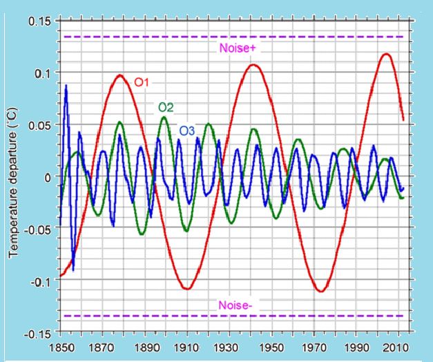
358 Figure
Figure5. 5.
(a)(a)
Three hypothesized
Three tidaltidal
hypothesized oscillations present
oscillations in GMST
present anomalies
in GMST at successively
anomalies higher higher
at successively
359 frequencies;
frequencies; (b)(b)
AnAn
equivalent deconstruction
equivalent deconstruction by Schlesinger [41], [41],
by Schlesinger reprinted by kind
reprinted permission
by kind of
permission of the
360 the Departmentofof
Department AtmosphericSciences
Atmospheric Sciencesatatthe
theUniversity
UniversityofofIllinois
IllinoisatatUrbana-Champagne
Urbana-Champagne on on behalf of
361 behalf of the
the late late Michael
Michael Schlesinger.
Schlesinger.
362 InInFigure
Figure5a:5a:Oscillation
Oscillation11isis aa segment
segment of the sine
of the sine curves
curves in
inFigures
Figures33andand4.4.When
Whenthe the
oscillation
363 oscillation decreases, the result is a ~30-year meridional regime and a hiatus in GMSTs. The 2004
decreases, the result is a ~30-year meridional regime and a hiatus in GMSTs. The 2004 turning point
364 turning point represents the timing of the beginning of the recent hiatus from the tidal approach and
represents the timing of the beginning of the recent hiatus from the tidal approach and the Figure by
365 the Figure by Schlesinger [39] seems to agrees with that timing.
Schlesinger [39] seems to agrees with that timing.
366 Oscillation 2 is the sum of two bidecadal-to-decadal tidal components (the 14.94- and 21.70-year
367 Oscillation
quarter-period 2 is the sum
'daughters' of theof59.75-
two bidecadal-to-decadal
and 86.81-year 'parent' tidal components
components) in T17(the 14.94-
Figure and
5; the two21.70-year
368 quarter-period ‘daughters’ of the 59.75- and
daughters can be seen in Figure 1 of the present paper. 86.81-year ‘parent’ components) in T17 Figure 5; the two
369 daughters can 3beisseen
Oscillation in Figure
obtained 1 of the present
by subtracting paper.
the above bidecadal-to-decadal variability from the
370 Oscillation
six-component 3 is obtained by subtracting
bidecadal-to-subdecadal variabilitythe
in above
Figure bidecadal-to-decadal
6 in the same source, variability
in order tofrom the
371 six-component bidecadal-to-subdecadal variability in Figure 6 in the same source,subdecadal
remove the duplicated bidecadal-to-decadal components. This generates the irregular in order to remove
372 temperature
the duplicated response in Oscillation 3 because
bidecadal-to-decadal the bidecadal-to-subdecadal
components. component
This generates the irregular amplitudes
subdecadal temperature
373 change
responsebetween zonal and3 meridional
in Oscillation because the regimes.
bidecadal-to-subdecadal component amplitudes change between
zonal and meridional regimes.
374 3.2. On the Timing and Duration of the Recent Hiatus
375 3.2. Lewandowsky
On the Timing et
andal.Duration of the40
[1] compiled Recent Hiatus
different assessments of the beginning and end of the
376 recent hiatus. Some of the assessed start and finish years were slightly ambiguous but the years
Lewandowsky et al. [1] compiled 40 different assessments of the beginning and end of the recent
377 centred on a few particular ones. Starting years for the hiatus ranged from 1993 to 2003, with the
hiatus. Some of the assessed start and finish years were slightly ambiguous but the years centred on
378 'most favoured' years being 1998 and 2000 (representing a total of about half of the assessed starting
a few particular ones. Starting years for the hiatus ranged from 1993 to 2003, with the ‘most favoured’
379 years), followed by 2001; the other years had a much smaller representation. End years for the recent
380 years
hiatus inbeing 1998 and 2000
the compilation (representing
ranged from 2008 to a 2013,
total ofwithabout
15 ofhalf ofthose
40 of the assessed starting
years assessed years),
to be 2012,followed
381 by 2001;bythe
followed other
9 for years
2013, then had a much
decreasing smaller
numbers forrepresentation. End The
2010, 2009 and 2008. years for the
median recent hiatus
beginning and in the
382 compilation ranged from 2008 to 2013, with 15 of 40 of those years assessed
end years were 2000 and 2012, giving a 12-year duration. However, the tidal hypothesis indicates to be 2012, followed by 9
383 for 2013,3.1)
(section then decreasing
that the presentnumbers for 2010,
meridional 2009began
regime and 2008. The and
in 2004 medianwillbeginning
continue and untilend years were
2034,
384 2000 and with
consistent 2012,the
giving a 12-year
~30-year duration.
meridional However, the tidal hypothesis indicates (Section 3.1) that the
timescale.
385 It seems
present there is no
meridional currently
regime agreed,
began expected
in 2004 or theoretical
and will continueduration for aconsistent
until 2034, hiatus. Thewith
~30-year
the ~30-year
386 durations for three
meridional timescale. hiatus episodes are consistent in the Schlesinger and Treloar deconstructions,
387 each episode
It seems representing
there is nothe coolingagreed,
currently half of aexpected
~60-year oscillation. If a duration
or theoretical generally forrecognized
a hiatus.hiatus
The ~30-year
388 isdurations
found to forhavethree
a 12-year duration and this is taken as the cooling half of a higher-frequency
hiatus episodes are consistent in the Schlesinger and Treloar deconstructions,
389 oscillation, then that oscillation would have a period around 24 years. Interestingly, the bidecadal
each episode representing the cooling half of a ~60-year oscillation. If a generally recognized hiatus is
390 component (Oscillation 2) in Figure 5a has a mean period of 21.7 years, since it is dominated by the
found to have a 12-year duration and this is taken as the cooling half of a higher-frequency oscillation,
391 21.70-year meridional 'daughter.’ The minimum and maximum in that curve corresponding to the
392 then thatinoscillation
medians would have
the Lewandowsky a period
et al. around
compilation 24 years.
occur duringInterestingly,
2005 and 2019. the Abidecadal component
conceivable
393 (Oscillation 2) in Figure 5a has a mean period of 21.7 years, since it
explanation for the discrepancy between the two sets of results may lie in the difficulty ofis dominated by the 21.70-year
394 meridional ‘daughter.’ The minimum and maximum in that curve
characterizing a decadal-scale hiatus in GMSTs in the presence of an accompanying ~60-yearcorresponding to the medians in
the Lewandowsky et al. compilation occur during 2005 and 2019. A conceivable explanation for the
discrepancy between the two sets of results may lie in the difficulty of characterizing a decadal-scaleClimate 2019, 7, 31 11 of 21
hiatus in GMSTs in the presence of an accompanying ~60-year oscillation and a rising background from
radiative forcing due to atmospheric GHGs. However, the possibility exists that we may encounter
a combination of both ~30- and ~11-year hiatus periods (the latter from bidecadal oscillations) in global
and ocean basin temperatures.
The possibility that El Niño events influence estimates of the timing of hiatus episodes is examined
in the Discussion section. However, tidal forcing is exogenous and essentially deterministic and should
not generate the hiatus as a stochastic process. Consequently, it should provide no uncertainty about
the hiatus start and finish if identified with times when the ~60-year curve enters and leaves its
meridional phase; the tidal turning points are consequently defined.
An interesting question is whether cooling from tidally-forced ocean energy redistribution and
heat uptake during the regime can now overcome the curvilinear temperature increase by radiative
forcing from increasing atmospheric concentrations of GHGs. Updating the T17 iteration procedure as
mentioned in the last section, the power function expression representing the curvilinear response to
the radiative forcing from increasing atmospheric GHG concentrations is amended to 3.65 × 10⁻⁷ ×
(t − 1851.5)2.87 , where t is the decimal year at a post-1851.5 time. The annual increase in the power
function expression at time t is the gradient, equal to about 1.05 × 10⁻⁶ × (t − 1851.5)1.87 and the
decadal change is ten times that. Mid-meridional regime times in Figures 3 and 5a are 1896.5, 1958.5 and
2019.0, which therefore imply respective decadal temperature increases from the curvilinear rise to be
0.013, 0.065 and 0.151 degrees C. In contrast, the mid-meridional regime decadal temperature decreases
in the solid curve in Figure 3 are in the range 0.08 to 0.1 degrees C. It is therefore clear that, while the
first two meridional regimes do produce a ~30-year cooling episode on this parameterization, the third
and subsequent meridional regimes would not (assuming GHG concentrations continue to increase);
the rise in radiative forcing from atmospheric GHG increases will override that cooling. The cooling
segments in Oscillation 2 of Figure 5a, representing a near-bidecadal contribution to GMSTs (from
14.94- and 21.70-year tidal components), are also of a magnitude that would be overridden in future by
the background curvilinear increase from GHG atmospheric concentrations.
GMSTs since 1850 have been simulated as the summation of (a) a power function expression
for the radiative forcing from atmospheric GHGs and (b) a three-fold recurrence of the ~60-year
oscillation derived from a parameterization of tidal forcing (the latter being essentially deterministic).
This is inconsistent with a view that the hiatus is generated stochastically. However, stochastic natural
fluctuations in sea surface temperatures may be important locally.
It has been noted (Section 1.1) that the recent GMST hiatus has been linked to contemporaneous
cool episodes in ocean basin oscillations such as the IPO, PDO and NAO. If the tidal approach to
GMSTs invokes the three multidecadal (59.75-, 86.81- and 186.0-year) components to explain the hiatus,
then the same three components should also be found in ocean basin oscillations. Each of these
is expected to include the 8-year lag associated with hypothesized zonal regime evaporation and
subsequent atmospheric rise of GHGs (Section 3.1). This is explored in the next sections.
3.3. An Interdecadal Pacific Oscillation (IPO) Reconstruction from an Antarctic Ice Core
Using piece-wise linear fit (PLF) and decision tree (DT) reconstruction methods, Vance et al. [46]
generated a near-1000-year IPO reconstruction from sea salt content in an ice core from the Law
Dome site in the Antarctic. With the timing of tidal maxima (2047.96 + 59.75n for the 59.75-year
component, 2047.96 + 86.81n for the 86.81-year component and 1926.20 + 186.0n for the 186.0-year
component, where n is a negative or positive integer), regression shows a significant zonal 59.75-year
component but much more significant meridional 86.81- and 186.0-year components, the latter with
probability p values of 5.4 × 10⁻²² and 10.9 × 10⁻²⁶ and with t statistics of −9.9 and +10.9 respectively.
The DT-median reconstruction is shown in Figure 6, with vertically scaled contributions from the
meridional components. Consistent with the Z–M formulation and equation (1), the sign of the cosine
function for the meridional 86.81-year component is negative and that for the meridional 186.0-year
cosine function is positive.Climate 2019, 7, 31 12 of 21
Climate 2018, 6, x FOR PEER REVIEW 12 of 21
444
445 Figure
Figure6. 6.Comparing the IPO
Comparing the IPOproxy
proxyofofVance
Vance et [45]
et al. al. [45]
withwith two vertically-scaled
two vertically-scaled meridional
meridional tidal
446 tidal oscillations.
oscillations.
447 Figure
Figure6 shows
6 showsnononotable
notablepresence
presenceofof~60-year oscillations.Rather,
~60-year oscillations. Rather,ititsuggests
suggestslonger
longer duration
duration
448 changes
changes in temperature,
in temperature,produced
produced byby
thethe
mix
mixof of
meridional
meridional 86.81- and
86.81- and186.0-year
186.0-yearoscillations.
oscillations.TheTheDT
449 DT shows
curve curve shows
visuallyvisually persuasive
persuasive agreement
agreement with 86.81-year
with 86.81-year extrema extrema afterand
after 1600 1600 and 186.0-year
186.0-year extrema
450 extrema
earlier andearlier and also that
also suggests suggests that the alternating
the alternating agreement agreement with 86.81-year
with 86.81-year minima minima
prior to prior to is
1600
451 1600 is reinforced by minima in the 186.0-year component. The possible transition in
reinforced by minima in the 186.0-year component. The possible transition in the interaction between the interaction
452 between
186.0- 186.0- andcomponents
and 86.81-year 86.81-year components coincides
coincides (perhaps (perhaps fortuitously)
fortuitously) with the time with the time of
(1550–1610)
453 an (1550–1610)
abrupt 10 ppm of an abrupt 10
decrease in ppm decrease
greenhouse incontent
gas greenhouse gasrecorded
[47] as content [47] asice
in an recorded in an
core from ice core
(again) Law
454 from (again) Law Dome. The high southern
◦ latitude (-66.8° S) of the Law Dome
Dome. The high southern latitude (−66.8 S) of the Law Dome site may help to explain the dominance site may help to
455 explain the dominance of meridional contributions. The roughly equal vertical scaling
of meridional contributions. The roughly equal vertical scaling for the two components in Figure 6 for the two
456 components in Figure 6 varies from the previously calculated relative amplitudes of 1 : 0.32 and the
varies from the previously calculated relative amplitudes of 1:0.32 and the reason may be a region- or
457 reason may be a region- or latitude-dependent one.
latitude-dependent one.
458 The two meridional components are anti-correlated in relation to their tidal maxima (as
The two meridional components are anti-correlated in relation to their tidal maxima (as evidenced
459 evidenced by the signs of the t statistics) and this will be observed for results in ocean basins in
by the signs of the t statistics) and this will be observed for results in ocean basins in following
460 following subsections. The reason for this anti-correlation is unclear but the pattern in the signs for
461 subsections. The reason for this anti-correlation is unclear but the pattern in the signs for cosine
cosine functions is explored in a broader context in Table 1 below.
functions is explored in a broader context in Table 1 below.
462 3.4.A Pacific Decadal Oscillation (PDO) Reconstruction
3.4. A Pacific Decadal Oscillation (PDO) Reconstruction
463 Gedalof et al. [48] used principal components analysis to find common modes of variance in five
464 Gedalof
climate et al. [48] used
reconstructions principal
around components
the North Pacific analysis
Basin thatto find
link common modes interdecadal
to extratropical of variance in
465 fivevariability.
climate reconstructions around the North Pacific Basin that link to extratropical
Using singular spectrum analysis, three eigenvectors were extracted, producing interdecadal
PDO
466 variability.
components with periods of around 23, 20 and 80 - 85 years. These components are shown PDO
Using singular spectrum analysis, three eigenvectors were extracted, producing in
467 components
Figures 7a–c, with periods with
overlapped of around 23,scaled
vertically 20 and
tidal80–85 years. with
components These components
periods areand
21.70, 18.60 shown
86.81 in
468 Figure
years7a–c,
withoverlapped
their respectivewithdefined
vertically scaled
phases. Thetidal components
respective with periods
expressions 21.70, 18.60are:
for the components and−0.2
86.81
469 years with their respective
cos[2π(t-2039.96)/21.70], −0.2defined phases. The respective
cos[2π(t-1918.20)/18.60] and −0.36expressions for the components
cos[2π(t-2047.96)/86.81]. The latter are:
470 −0.2 cos[2π(t −
component 2039.96)/21.70],
incorporates −0.2 lag
the 8-year cos[2π(t − 1918.20)/18.60]
derived and −0.36 cos[2π(t
for the three multidecadal − 2047.96)/86.81].
components in T17, to
471 Theaccount for the timeincorporates
latter component for GHGs tothe migrate
8-yeartolag
thederived
upper foratmosphere.
the three The first two, components
multidecadal like all other in
472 components
T17, to accountderived in T02
for the time forand T17, to
GHGs aremigrate
assumed to to actupper
the at theatmosphere.
ocean surfaceTheandfirst
assigned a zero
two, like all lag
other
473 time. See section
components derived 3.1inabove.
T02 and T17, are assumed to act at the ocean surface and assigned a zero lag
time. See Section 3.1 above.Climate 2019, 7, 31 13 of 21
Climate 2018, 6, x FOR PEER REVIEW 13 of 21
474
475
476
477 Figure 7. A7.comparison
Figure A comparison of of
derived
derivedPDO
PDOandandtidal
tidal components. Blue:PDO
components. Blue: PDO eigenvector
eigenvector modes
modes foundfound
478 by Gedalof
by Gedalof et al.
et al. [48].
[48]. Red:Tidal
Red: Tidalcomponents
components derived
derived ininT02
T02and
andT17,
T17,vertically
verticallyscaled. TheThe
scaled. figures
figures
479 compare
compare respective
respective eigenvector
eigenvector modes
modes andand tidal
tidal curves
curves having
having periods:(a)
periods: (a)~23
~23and
and21.70
21.70 years;
years; (b)
(b) ~20
480 ~20 and 18.60 years; and (c) ~80 or ~85 and 86.81 years. SSA data for the three modes
and 18.60 years; and (c) ~80 or ~85 and 86.81 years. SSA data for the three modes are used by kindare used by kind
481 permission
permission of Prof.
of Prof. Gedalof..
Gedalof.Climate 2019, 7, 31 14 of 21
The scaling in these Figures incorporates sign-reversal for all three tidal cosine components.
This implies that maxima in tidal forcing (times when close perigee tends to occur at new moon)
corresponds to lower temperatures and perhaps greatest upwelling. The reference date for the
86.81-year meridional component was 2047.96, which incorporates an 8-year lag (with respect to
2039.96); the 18.60- and 21.70-year components have reference dates of 1918.20 and 2039.96, therefore
with no lag time, for reasons given earlier. In sum, the Gedalof et al. curves can be represented
by the 21.70- and 18.60-year ‘daughters’ of the 86.81- and 186.0-year meridional ‘parents’ (Figure 1),
along with the meridional 86.81-year component itself.
The last two sets of curves (Figure 7b,c) are in close accord; the correspondence in 7c is rather
stunning and supports the eight-year lag for the three multidecadal tidal oscillations (see Section 3.1).
However, the first set (7a) has poor agreement and Gedalof et al. [48] remarked on the weakness of the
~23-year mode prior to 1875 when the five proxies correlated poorly, commenting that the PDO has not
been a coherent structure over time. A discrepancy in low frequency behaviour between PDO proxies
has also been noted by Kipfmueller et al. [49]. Multidecadal changes in their PDO proxy were noted
by MacDonald and Case [50] and changes were also observed in the Law Dome PDO proxy above.
3.5. Multidecadal Correlation Patterns in Ocean Basin Oscillations
In spite of the inconsistencies reported above, correlations of the three multidecadal tidal
components (186.0-, 86.81- and 59.75-year) with multiple spatially-diverse proxies in the Pacific
and Atlantic basins show a generally similar pattern (Table 1). Several data sets in Table 1 have
durations too short in relation to the lengths of the tidal periods to expect consistent results but there is
nevertheless a tendency toward a probability p-value pattern of 186.0 positive, 86.81 negative and 59.75
positive. Gedalof et al. [48] noted that paleo-proxy networks capture large-scale ocean-atmosphere
interactions better than spatially restricted single proxies and the pattern emerging from this suite of
regression results may support that finding.
Table 1. The probability p-value pattern for the 186.0-, 86.81- and 59.75-year tidal components in
regressions of temperature variability in Pacific and Atlantic ocean basins and including the sense
(positive or negative) of the correlation. Key: quadruple sign (+ or −), p < 10−10 ; triple sign, p < 10−5 ;
double sign, p < 0.05; single sign, correlation not significant. N.B. the proxy data for Shen et al. [51] and
for MacDonald and Case [50] were linearly detrended before regression.
Data Length
Oscillation Data Source 186.0 yr 86.81 yr 59.75 yr
(yr), Frequency
Vance et al. PLF ++++ ––– +
IPO 998, yearly
[DT-median] [45] [+ + + + ] [– – – –] [+ +]
IPO-TPI Henley et al. [52] 141, monthly ++ –––– +
PDO NOAA / NCEI [53] 163, monthly ++ –– +++
PDO Shen et al. [51] 529, yearly – ++ ++
PDO Biondi et al. [54] 331, yearly – – ++
PDO Gedalof et al. [48] 157, yearly ++ ––– ++
PDO Gedalof and Smith [55] 385, yearly – – –
PDO MacDonald and Case [50] 1004, yearly ++ + ++
NAO Jones et al. [56] 177, yearly + –––– +++
NAO Vinther et al. [57] 726, yearly + – ++
NAO Luterbacher et al. [58] 491, yearly ++ –– ++
NAO Glueck and Stockton [59] 525, yearly + –––– ++
NAO Cook et al. [60] 580, yearly + –– –You can also read