Vertically-resolved observations of Jupiter's quasi-quadrennial oscillation from 2012 to 2019
←
→
Page content transcription
If your browser does not render page correctly, please read the page content below
Vertically-resolved observations of Jupiter’s quasi-quadrennial oscillation from 2012
                                                                                      to 2019

                                                                     R. S. Gilesa,∗, T. K. Greathousea , R. G. Cosentinob,c , G. S. Ortond , J. H. Lacye
                                                                                         a Southwest Research Institute, San Antonio, TX, USA
                                                                                     b   NASA Goddard Spaceflight Center, Greenbelt, MD, USA
                                                                     c CRESST II and Department of Astronomy, University of Maryland, College Park, MD, USA
                                                                         d Jet Propulsion Laboratory / California Institute of Technology, Pasadena, CA, USA
                                                                                            e University of Texas at Austin, Austin, TX, USA
arXiv:2006.15247v1 [astro-ph.EP] 27 Jun 2020

                                               Abstract
                                                 Over the last eight years, a rich dataset of mid-infrared CH4 observations from the TEXES instrument at IRTF has been
                                               used to characterize the thermal evolution of Jupiter’s stratosphere. These data were used to produce vertically-resolved
                                               temperature maps between latitudes of 50◦ S and 50◦ N, allowing us to track approximately two periods of Jupiter’s quasi-
                                               quadrennial oscillation (QQO). During the first five years of observations, the QQO has a smooth sinusoidal pattern with
                                               a period of 4.0±0.2 years and an amplitude of 7±1 K at 13.5 mbar (our region of maximum sensitivity). In 2017, we
                                               note an abrupt change to this pattern, with the phase being shifted backwards by ∼1 year. Searching for possible causes
                                               of this QQO delay, we investigated the TEXES zonally-resolved temperature retrievals and found that in May/June
                                               2017, there was an unusually warm thermal anomaly located at a latitude of 28◦ N and a pressure of 1.2 mbar, moving
                                               westward with a velocity of 19±4 ms-1 . We suggest that there may be a link between these two events.
                                               Keywords: Jupiter; Atmospheres, structure; Infrared observations; Spectroscopy

                                               1. Introduction                                                    so there is a phase offset between different pressure levels
                                                                                                                  and a vertical wind shear that alternates between posi-
                                                  Long-term observations of Jupiter have shown peri-              tive and negative. On both Earth and Jupiter, the mean
                                               odic variations in the planet’s stratospheric temperatures.        zonal flow can be assumed to be in approximately hydro-
                                               Between 1980 and 2001, 7.8-μm images of Jupiter from               static and geostropic balance (Leovy et al., 1991), which
                                               NASA’s Infrared Telescope Facility (IRTF) were used to             means that the vertical wind shear and the horizontal tem-
                                               track the brightness temperature of Jupiter’s atmosphere           perature gradient are coupled through the thermal wind
                                               in the 10–20 mbar region (Orton et al., 1991; Leovy et al.,        equation (Baldwin et al., 2001). Unlike on the Earth, it
                                               1991; Friedson, 1999; Simon-Miller et al., 2006). These ob-        is difficult to make direct wind measurements in Jupiter’s
                                               servations showed an oscillation in the equatorial and low-        stratosphere, but it is possible to study the QQO’s signa-
                                               latitude regions of the planet with a period of ∼4 years; the      ture and evolution by observing changes in the tempera-
                                               stratospheric temperatures oscillate between having a local        ture field.
                                               maximum at the equator and local minima at planetocen-
                                               tric latitudes of ±13◦ , and having a local minimum at the            Despite being an equatorial phenomenon, the QBO has
                                               equator and local maxima at planetocentric latitudes of            a significant impact on the dynamics of the Earth’s atmo-
                                               ±13◦ . This phenomenon was named the quasi-quadrennial             sphere at all latitudes; this includes affecting the strength
                                               oscillation (QQO) by Leovy et al. (1991), who noted its re-        of Atlantic hurricanes and the breakdown of the winter-
                                               semblance to the quasi-biennial oscillation (QBO) that is          time stratospheric polar vortices (Baldwin et al., 2001).
                                               seen in the Earth’s stratosphere.                                  The QQO may also be an important factor in Jupiter’s
                                                  The QBO is a quasi-periodic oscillation in the Earth’s          weather patterns, and close monitoring of the QQO phase
                                               stratospheric zonal mean winds at tropical latitudes (Bald-        pattern is required to make any correlations with observed
                                               win et al., 2001). At a given pressure level, the equato-          dynamical changes. Careful analysis of the QQO also
                                               rial wind direction oscillates between easterly and west-          provides insight into the waves that are thought to drive
                                               erly with a mean period of 28 months. The easterly and             the phenomenon. The Earth’s QBO is driven by the ab-
                                               westerly wind regimes propagate downwards with time,               sorption of vertically-propagating atmospheric waves that
                                                                                                                  break and deposit their zonal momentum at a critical level
                                                                                                                  that is determined by the background zonal flow (Baldwin
                                                 ∗ Corresponding author                                           et al., 2001). For the Earth, Dunkerton (1997) showed that
                                                   Email address: rgiles@swri.edu (R. S. Giles)                   a combination of Kelvin, Rossby-gravity, inertia-gravity,
                                               Preprint submitted to Icarus                                                                                       June 30, 2020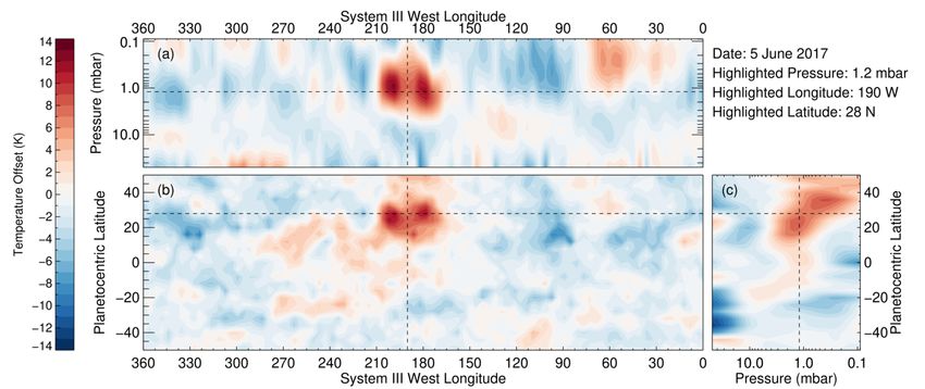
and smaller-scale gravity waves are required to reproduce          TEXES/IRTF for approximately eight years, which cor-
observed winds and temperatures. Similar mechanisms                responds to two cycles. These data allow us to look for
have been proposed as the driving forces behind Jupiter’s          additional variability superimposed on top of the QQO. In
QQO, and observations play an important role in con-               2015–16, an unusual disruption to the Earth’s QBO was
straining atmospheric models.                                      noted by Osprey et al. (2016) and Newman et al. (2016).
   The first models of the QQO were developed by Fried-            The exact causes of this event are still unclear, but both
son (1999) and Li and Read (2000), who were both able to           studies suggest it may be due to intrusion of Rossby waves
reproduce QQO-like phenomena within mechanistic mod-               from the winter hemisphere into the equatorial region of
els of Jupiter’s atmosphere; Li and Read (2000) sug-               the planet. Like Jupiter, Saturn also has an oscillation
gested that equatorial oscillations could be produced us-          in the equatorial stratosphere, known as Saturn’s Semi-
ing a combination of planetary-scale waves, while Friedson         Annual Oscillation (SSAO), and this has been observed to
(1999) implemented a flat-spectrum gravity wave drag pa-           be disrupted by a large long-lasting storm in the northern
rameterization and compared the effects of gravity waves           mid-latitudes (Fletcher et al., 2017a).
and planetary-scale waves, finding that small-scale, short-           In this paper, we present an updated vertically resolved
period gravity were better able to drive a QQO-like phe-           time series of Jupiter’s QQO covering the 2012–2019 time
nomenon. However, these studies were limited by the ob-            period. We find that after five years of smoothly vary-
servations that were available at the time. The 7.8-μm             ing sinusoidal behaviour, there was a change in the QQO
broad-band imaging campaign provided a valuable dataset            behaviour in 2017, and we use our spatially resolved obser-
over a long timeframe, but was limited to a single pressure        vations to show that this occurred in conjunction with a
range and did not have any sensitivity to vertical varia-          localized stratospheric thermal anomaly. The TEXES ob-
tions in the thermal profile.                                      servations and the data reduction process are described in
   More recent studies of Jupiter’s QQO have made use of           Section 2 and the radiative transfer model is presented in
spacecraft data from Voyager IRIS (Simon-Miller et al.,            Section 3. The long-term QQO observations and the 2017
2006) and Cassini CIRS (Flasar et al., 2004; Simon-Miller          disruption are discussed in Section 4 and the conclusions
et al., 2006). Both of these instruments provide spectro-          are summarized in Section 5.
scopic observations of Jupiter, allowing vertical tempera-
ture profiles to be retrieved in the stratosphere. This ver-
tical information is an important addition to the studies          2. Observations
of the QQO, but as the spacecraft observations were ob-
                                                                   2.1. TEXES observations
tained during flybys of Jupiter, they were each restricted
to short timeframes and cannot be used to study how the               Between 2012 and 2019, high-resolution mid-infrared
QQO varies with time.                                              observations of Jupiter were made with the TEXES instru-
   In order to improve our three-dimensional understand-           ment, mounted at the 3-m NASA Infrared Telescope Fa-
ing of the QQO and to inform future modeling efforts, we           cility. Data were obtained during eighteen observing runs,
began a long-term study of Jupiter’s stratospheric tem-            summarized in Table 1. TEXES is a cross-dispered grating
peratures in 2012, using the Texas Echelon Cross Echelle           spectrograph that covers wavelengths of 4.5–25 μm in the
Spectrograph (TEXES, Lacy et al., 2002), which operates            mid-infrared, with a resolving power between 4,000 and
as a visitor instrument at the IRTF. TEXES provides high-          80,000 depending on the mode of operation. The scan-map
resolution (R=80,0000) spectroscopy of line profiles, which        mode of TEXES produces spectral datacubes (two spatial
allows us to vertically resolve the temperature structure in       dimensions and one spectral dimension) of extended ob-
Jupiter’s stratosphere to a greater degree than was possi-         jects by stepping the slit across the sky perpendicular to
ble with the lower resolution Voyager IRIS and Cassini             the slit length.
CIRS observations. After the first complete cycle was ob-             In order to study Jupiter’s stratospheric temperatures,
served (2012–2016), the data were used to constrain a new          we used observations centered at 1247.5 cm-1 (8.02 μm),
General Circulation Model (GCM) analysis by Cosentino              with a spectral bandpass of ∼7 cm-1 . This spectral range
et al. (2017). The TEXES observations showed that the              covers six strong P-branch lines of the CH4 ν4 band, which
QQO extends upwards to lower pressures (∼2 mbar) than              is centered at 1306 cm-1 (Brown et al., 2003). TEXES was
previously known, and that there is a smooth sinusoidal            used in its highest spectral resolution mode (R=80,000),
transition between maxima and minima over a large range            which means that these lines are spectrally resolved. CH4
of pressures. Cosentino et al. (2017) concluded that high-         is homogeneously mixed in Jupiter’s stratosphere, and its
frequency gravity waves are significant contributors of mo-        abundance is well known. Variations in the shapes of CH4
mentum to the QQO, agreeing with earlier results from              emission lines are due to temperature variations alone and
Friedson (1999). In particular, Cosentino et al. (2017)            these emission lines therefore provide a direct measure-
found that a stochastic gravity wave drag parameteriza-            ment of Jupiter’s stratospheric temperature. At the center
tion, representative of an atmosphere with convection, is          of the strong emission lines, the atmosphere becomes opti-
better able to model the observations.                             cally thick at high altitudes in the stratosphere, so we are
   We have now been observing Jupiter’s QQO with                   sensitive to temperatures at those high altitudes. In the
                                                               2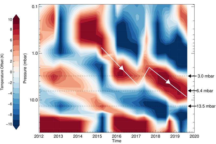
wings of those strong lines, or in the center of weaker lines,       front of instrument aperture prior to each set of observa-
the atmosphere does not become opaque until a lower al-              tions. The noise of each spectral data point was calculated
titude, and so we can probe deeper into the stratosphere.            following the method described for TEXES observations
By simultaneously modeling the 1244–1251 cm-1 spectral               in Greathouse et al. (2011).
range, we are able to retrieve the vertical temperature pro-            The pipeline-reduced data products were then geometri-
file in the 0.1–30 mbar pressure region.                             cally calibrated, cylindrically projected and co-added. The
   Three-dimensional temperature maps covering the                   scan parameters were used to calculate the shape of the
50◦ S–50◦ N latitude range were built up by using the                planet’s limb, which was then fitted to each observation
TEXES scan-map mode. We oriented the slit along the ce-              by eye. This allows each pixel to be assigned a latitude
lestial north-south direction and scanned across the planet          and longitude. The Doppler shift of the spectrum was cal-
from west to east. We used a step size of 0.700 (half the            culated for each pixel, comprising both a component due to
width of the slit) and observations of sky were included at          the Earth-Jupiter velocity and a position-dependent com-
the beginning and end of each scan to aid with sky subtrac-          ponent due to Jupiter’s rotation (zonal wind speeds are
tion. In the high-resolution observing mode, the TEXES               negligible in comparison); this Doppler shift was removed
slit length is 600 , which is considerably smaller than the          for each pixel, shifting the Jovian spectrum into the rest
diameter of Jupiter (see Table 1). In order to cover the             frame. The observations were then binned according to
entire 50◦ S–50◦ N latitude range, we therefore performed            airmass and then projected onto a latitude-longitude grid;
multiple scans with different north-south offsets. This ob-          this allows multiple scans to be co-added to produce a sin-
serving sequence was repeated continuously for ∼6 hours              gle data cube per airmass bin.
on a single night; due to Jupiter’s rotation period of 10
hours, this provides coverage of over half of the planet.            3. Spectral modeling
When possible, observations on a subsequent night were
then used to complete the global map. Table 1 shows that                The TEXES spectra were modeled using a radiative
we were able to obtain full longitudinal coverage at the             transfer and retrieval code that has previously been used
equator on the vast majority of the observing runs.                  to model the stratospheres of Saturn (Greathouse et al.,
   At 1247.5 cm-1 , the diffraction limit at the 3-m IRTF            2005) and Neptune (Greathouse et al., 2011). The code is
is 0.700 , which is comparable to the typical seeing at the          made up of a line-by-line radiative transfer code that cal-
telescope. For the angular diameters provided in Table 1,            culates the theoretical spectrum for a given atmospheric
this is equivalent to a spatial resolution of ∼2◦ latitude           profile and an optimal estimation retrieval code that uses
at the equator. In the longitudinal direction, the 1.400 slit        a Levenberg-Marquardt approach to iteratively adjust the
width leads to a spatial resolution of ∼4◦ longitude.                atmospheric parameters and achieve an optimal fit be-
   Our long-term observing program was designed to study             tween the theoretical spectrum and the observed spec-
both long- and short-term variability in Jupiter’s strato-           trum (Rodgers, 2000). The code is described in greater
spheric temperatures. In order to track the long-term                depth in Greathouse et al. (2011).
trends in temperature, observations were made on sev-                   For this study, Jupiter’s atmosphere was divided into 95
eral observing runs per year. These runs were nomi-                  levels between 4 bar and 1 × 10⁻⁷ bar, equally spaced in
nally planned as pairs with a 1-month spacing about each             log(p). The vertical distribution of CH4 was obtained from
quadrature. Observing near quadrature ensured a suffi-               the photochemical model of Moses et al. (2005), which
ciently large Doppler shift between Earth and Jupiter to             takes into account both eddy mixing and molecular diffu-
separate the terrestrial and Jovian CH4 lines (see Table 1           sion. The line data for 12 CH4 , 13 CH4 and 12 CH3 D were
for the Doppler velocity during each run). In order to mea-          obtained from the HITRAN molecular database (Roth-
sure short-term variability, we aimed to repeat our obser-           man et al., 2005), and the temperature dependence of the
vations at both the beginning and end of a given observing           line widths in an H2 atmosphere was obtained from Mar-
run, however weather conditions meant that this was not              golis (1993). Collision induced absorption data for H2 -
always possible. In total, these observations provide com-           H2 , H2 -He and H2 -CH4 were included from Orton et al.
parisons over 1-week, 1-month and 4-month intervals.                 (2007), Borysow et al. (1988) and Borysow and Frommhold
                                                                     (1986) respectively. We assume local thermodynamic equi-
                                                                     librium (LTE) at all pressure levels; our observations are
2.2. Data reduction
                                                                     primarily sensitive to pressures in the 0.1–30 mbar range,
  The individual scans of Jupiter were each reduced us-              and the transition between LTE and non-LTE does not
ing the data reduction pipeline described in Lacy et al.             occur until ∼1 μbar (Drossart et al., 1999).
(2002). This software performs flat fielding and sky sub-               The a priori vertical temperature profile is based on the
traction, and then removes instrumental geometric optical            model described in Moses et al. (2005). This profile was al-
distortions. Wavelength calibration was achieved by us-              lowed to vary in the retrievals, in order to fit the TEXES
ing telluric absorption lines and radiometric calibration            spectra. The temperature is retrieved at each of the 95
was achieved by using the measured radiance of a room                pressure levels and a correlation length of 1 scale height
temperature blackbody that is automatically placed in                is used to prevent unphysically sharp deviations between
                                                                 3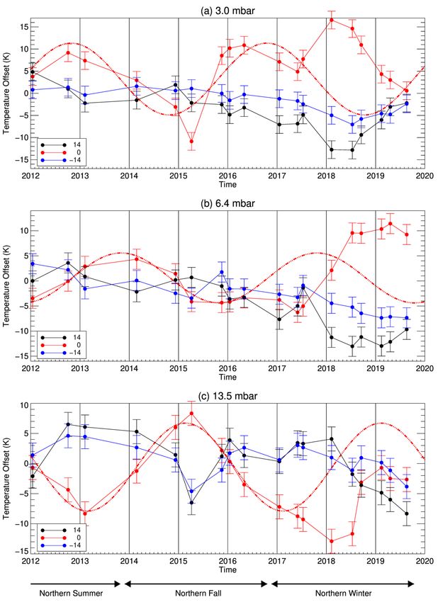
Longitudinal         Angular          Earth-Jupiter       Sub-solar        Heliocentric
                    Date         coverage at the       diameter           velocity        planetocentric      distance
                                   equator (%)         (arcsec)            (km/s)          latitude (◦ )       (AU)
                 Jan 2012               72                41                  28               3.07             4.98
                 Sep 2012              100                44                 -24               2.92             5.04
                 Feb 2013              100                42                  27               2.68             5.08
                 Feb 2014              100                43                  23               1.44             5.21
                 Dec 2014               78                41                 -25               0.23             5.31
                 Mar 2015              100                41                  25               -0.26            5.35
                 Nov 2015              100                34                 -26               -1.17            5.41
                 Jan 2016              100                41                 -24               -1.39            5.42
                 Apr 2016              100                41                  24               -1.76            5.44
                 Jan 2017              100                37                 -28               -2.51            5.46
                 May 2017              100                41                  23               -2.79            5.45
                 Jul 2017               61                36                  27               -2.86            5.45
                 Feb 2018              100                37                 -29               -3.07            5.43
                 Jul 2018              100                40                  25               -3.07            5.40
                 Sep 2018              100                34                  22               -3.02            5.38
                 Feb 2019              100                35                 -26               -2.84            5.34
                 Apr 2019              100                42                 -23               -2.72            5.32
                 Aug 2019              100                40                  25               -2.44            5.28

Table 1: Summary of IRTF observing runs contributing to this study: the month and year, the longitudinal coverage obtained over the
course of the observing run, Jupiter’s angular diameter as observed from the Earth, the Doppler velocity, the sub-solar Jovian latitude and
the distance of Jupiter from the sun.

adjacent levels. Figure 1 shows an example of a fitted spec-             spectrum for each latitude (2◦ bins) and airmass (four bins,
trum and a retrieved temperature profile for data obtained               covering airmasses of 1–5). For each latitude, the retrieval
on 17–18 November 2015. Figure 1(a) shows the TEXES                      code was used to simultaneously fit the different airmass
spectrum in black, along with the best-fit model spectrum                spectra, in order to produce a final vertical temperature
in red. The gap in the data at 1247.7 cm-1 is due to the                 profile for that latitude. Combining the vertical tempera-
presence of a strong telluric line. Figure 1(b) shows the                ture profiles for each latitude produces a two-dimensional
corresponding retrieved vertical temperature profile along               temperature map. These zonally-averaged maps are the
with the a priori temperature profile. The error bars shown              focus of Sections 4.1 and 4.2.
in Figure 1(b) represent the formal uncertainty in the re-                  The observational data were also used to produce
trieval. They are a minimum at ∼13 mbar, the pressure                    zonally-resolved three-dimensional maps. These were gen-
level of maximum sensitivity. As the pressure increases,                 erated by retrieving the vertical temperature profile at
the formal error bars also increase, but do not fully cap-               each longitude and latitude point, instead of averaging
ture the dependence on any assumed model parameters                      across the longitudinal dimension. This allows us to search
in the deeper atmosphere. We consider the retrievals to                  for spatially-localized thermal anomalies, as shown in Sec-
be robust in the 0.1–30 mbar region. Within this region,                 tion 4.3.
the formal error bars are ∼1.5 K; in the subsequent sec-                    An example of a retrieved zonally-averaged temperature
tions, we adopt a more conservative error of 2 K to include              map from 17–18 November 2015 is shown in Figure 2(a).
systematic effects (Cosentino et al., 2017).                             The dashed lines in the figure show latitudes of 14◦ S, 0◦
   The radiative transfer and retrieval code was applied to              and 14◦ N, the locations of the main equatorial QQO sig-
all of the observations described in Section 2 in order to               nature and the anti-phase components. Figure 2(a) shows
produce both two-dimensional and three-dimensional tem-                  a clear vertical oscillation in temperature at the equator,
perature maps for each observing date. As the QQO is an                  with a strong local minimum (relative to the off-equatorial
oscillation pattern in the global-scale wind field, we are pri-          ±14◦ temperatures) at approximately 8 mbar and strong
marily interested in the two-dimensional, zonally-averaged               local maxima at approximately 2 mbar and 20 mbar. This
temperature maps. As described in Section 2, the TEXES                   is highlighted by Figure 2(b), which shows the tempera-
spectral data were binned according to latitude, longitude               tures as a function of latitude for 2 mbar and 8 mbar.
and Jovian airmass. Data obtained from several nights on                    This vertical oscillation is a signature of the QQO; as
each observing run were then co-added to provide as com-                 time passes the local maxima and minima at the equator
plete longitudinal coverage as possible. The data were then              move to deeper pressure levels. To study this, compara-
averaged across all longitudes, in order to produce a single             ble temperature maps were made for each observing run
                                                                    4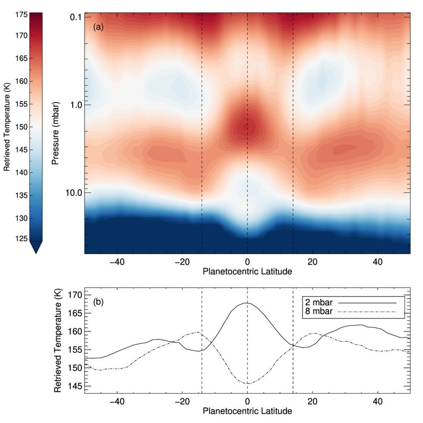
0.5                                                                                   0.1
                                                                   (a)                                                                                   (b)
                                                             0.4

                                                             0.3

                        Radiance (erg s−1cm−2sr−1(cm−1)−1)
                                                             0.2

                                                                                                                                Pressure (mbar)
                                                             0.1                                                                                   1.0
                                                             0.0
                                                             1244.5      1245.0   1245.5   1246.0    1246.5   1247.0   1247.5
                                                             0.5
                                                             0.4

                                                             0.3                                                                                  10.0
                                                             0.2

                                                             0.1
                                                             0.0
                                                             1247.5      1248.0   1248.5   1249.0    1249.5   1250.0   1250.5                       100        120  140      160   180
                                                                                      Wavenumber (cm−1)                                                         Temperature (K)

Figure 1: (a) An example of a zonally-averaged equatorial TEXES spectrum from 17–18 November 2015 (black) along with the best-fit model
spectrum (red). The spectrum is split into two frames to make the features more clear. (b) Corresponding vertical temperature profile (red),
along with the a priori temperature profile (black).

conducted in 2012–2019 (Table 1). The evolution of the                                                            Allen and Sherwood, 2007); positive (eastward/westerly)
stratospheric temperatures with time is described and dis-                                                        vertical wind shear in the QBO is correlated with warm
cussed in Section 4. Section 4.1 discusses the evolution                                                          equatorial anomalies (Pascoe et al., 2005).
of Jupiter’s QQO over the 2012-2017, while Section 4.2                                                               Figure 4 presents the QQO data for three different pres-
discusses an apparent disruption in the QQO pattern in                                                            sure levels: 3.0 mbar, 6.4 mbar and 13.5 mbar. The red
2017.                                                                                                             data points correspond to the same equatorial data that
   We note that Figure 2 also shows other interesting phe-                                                        are shown in Figure 3. The dashed lines in Figure 3 high-
nomena, such as a vertical temperature oscillation in the                                                         light the three pressure levels used in Figure 4. Along-
mid-latitudes (±20–30◦ ). However, no oscillation is ob-                                                          side the equatorial temperature offsets, we also present
served at these latitudes and there is therefore no clear                                                         the temperature offsets for 14◦ N (black) and 14◦ S (blue).
link with the QQO. Analysis of the retrieved mid-latitude                                                            The long-term 7.8-μm images that were first used to
temperatures is therefore outside the scope of this paper.                                                        identify the QQO (Orton et al., 1991; Leovy et al., 1991)
                                                                                                                  are sensitive to the 10–20 mbar pressure range; Figure 4(c)
4. Results and discussion                                                                                         therefore provides the best comparison with those results.
                                                                                                                  This pressure levels also corresponds to the region of max-
4.1. Behavior of the QQO in 2012–2017                                                                             imum sensitivity for the TEXES data. Figure 4(c) shows
   Figure 3 shows the time series of Jupiter’s equatorial                                                         a clear sinusoidal pattern for the first five years of the
temperature oscillation during the entire 2012–2019 ob-                                                           data collection (2012–2017). Fitting a sine curve to the
servation period. All observations from a given observing                                                         pre-2017 red equatorial data results in a period of 4.0±0.2
run are combined into a single zonally-averaged tempera-                                                          years; the fitted curve is shown by the red dashed line. The
ture retrieval. The retrieved temperatures are the average                                                        amplitude of this fitted oscillation at 13.5 mbar is 7±1 K.
from the 2◦ S–2◦ N latitude range and the temperature off-                                                        The 14◦ N and 14◦ S temperatures also show a roughly si-
set at each pressure level is defined as the zonally-averaged                                                     nusoidal pattern at 13.5 mbar for the first five years, which
temperature relative to the average of the maximum and                                                            is in anti-phase to the equatorial temperatures and has a
minimum temperature in 2012–2016 (corresponding to a                                                              comparable magnitude. This agrees with previous IRTF
complete, unperturbed oscillation).                                                                               observations which showed that the 7.8-μm brightness is
   Figure 3 is analogous to the time-height diagrams of the                                                       anti-correlated between the equator and ±13◦ (Friedson,
Earth’s QBO, as seen in e.g. Naujokat (1986). As with the                                                         1999).
QBO, the QQO consists of downward propagating warm                                                                   As previously discussed in Cosentino et al. (2017), the
and cool regions, causing the temperature at a given pres-                                                        vertically-resolved TEXES observations show for the first
sure level to oscillate with time. With the Earth’s QBO,                                                          time that Jupiter’s QQO extends to lower pressures. This
the time taken for the pattern to repeat is approximately                                                         can be clearly seen in Figure 3, which shows the diagonal,
two years, and for Jupiter’s QQO, the period is approx-                                                           downward propagating pattern extend between ∼1 mbar
imately four years. On Earth, wind speeds can be mea-                                                             and ∼20 mbar. At pressures less than 1 mbar, no clear
sured directly and so time-height diagrams are typically                                                          oscillation is observed, although it should be noted that
presented in terms of winds. However, the wind shear                                                              our sensitivity begins to decrease at these pressures.
and temperatures are coupled via the thermal wind equa-                                                              Figures 4(a) and (b) show how the QQO oscillations ap-
tion (which for Earth remains valid deep into the tropics,                                                        pear at pressures of 3.0 mbar and 6.4 mbar. The 2012–2017
                                                                                                              5
Figure 2: (a) Example of a zonally-averaged retrieved temperature map from 17–18 November 2015. The vertical dashed lines show latitudes
of 14◦ S, 0◦ and 14◦ N, the three latitudes that are shown in Figure 4. (b) Slices through (a) at two different pressures levels representing a
local maximum at the equator (2 mbar) and a local minimum at the equator (8 mbar).
6Figure 3: Time series of Jupiter’s QQO from 2012–2019 as a function of pressure and time. The retrieved temperatures are from Jupiter’s
equator (2◦ S–2◦ N) and the temperature offset for each pressure level is defined as the zonally-averaged temperature relative to the average
of the maximum and minimum temperature during the first four years of data (corresponding to a complete, unperturbed oscillation). The
dashed black lines highlight the 3.0-mbar, 6.4-mbar and 13.5-mbar pressure levels that are shown in Figure 4. The white line shows an
apparent disruption in the descending warm branch.
data in these figures show that the equatorial temperatures after the previous local maximum. When the equatorial
at these lower pressures still exhibit an approximately si- temperatures start to decrease again, they are ∼1 year
nusoidal pattern. The dashed red lines in Figures 4(a) and behind schedule.
(b) show the best-fit sine curve to the 2012–2017 equatorial Figure 4 also shows how the off-equatorial tempera-
data, assuming the same 4.0-year period derived from Fig- tures vary from 2017 onward. Figure 4(c) shows that the
ure 4(c). At 6.4 mbar, the oscillation is still a smooth sine ±14◦ temperatures broadly continue in anti-phase with the
wave; at 3.0 mbar, it appears to be more ‘sawtooth’. At equatorial temperatures. In particular, it can be seen that
these higher altitudes, any oscillation in the off-equatorial the 14◦ N temperature peaks in early 2018, at the same
temperatures is significantly weaker than at 13.5 mbar. time as the equatorial temperatures reach their delayed
minimum. The off-equatorial results shown in Figures 4(b)
4.2. Disruption of the QQO in 2017 and (c) also show a change in 2017. Before 2017, the ±14◦
temperature offsets are relatively flat. From mid-2017 on-
The temperature offsets in 2012–2017 appear to show a
ward, the 14◦ S temperatures continue to be mostly flat,
‘typical’ QQO pattern, consisting of a smoothly varying
but the 14◦ N temperatures show a stronger inverse corre-
sinusoidal oscillation with a period of ∼4 years. However,
lation with the equatorial temperatures.
Figures 3 and 4 show that there is a phase-shift disruption
to this pattern in mid-2017. Further insight into how the equatorial temperatures
The equatorial data, shown in red in Figure 4(c), show evolved over this time period can be obtained from Fig-
that the temperatures continue to decrease in late 2017 / ure 3. The solid white line shows the motion of the de-
early 2018, rather than following the 4-year-period sinu- scending warm branch of the QQO. In 2017, this warm
soidal pattern shown by the dashed red line. This leads to branch undergoes an abrupt upward displacement. This
the minimum in the equatorial 13.5-mbar temperature oc- has the effect of ‘delaying’ the QQO by ∼1 year at the 3.0-
curring ∼1 year later than expected. Similar shifts can be mbar, 6.4-mbar and 13.5-mbar pressure levels, as shown
observed in Figures 4(a) and (b). In Figure 4(b), the equa- in Figure 4. The upwards displacement of the descending
torial data lags ∼1 year behind the nominal sinusoid from warm branch coincides with an abrupt, short-lived warm-
2017 onwards. In Figure 4(a), the change is even more ing at high altitudes (0.2–2 mbar).
stark. In 2017–2018, we would expect the equatorial 3- The QQO disruption observed in Figures 3 and 4 bears
mbar temperatures to be decreasing, reaching a minimum some similarities to the disruption of the Earth’s QBO that
in late 2018. Instead, the temperatures start to decrease was observed in 2015–2016 (Osprey et al., 2016; Newman
as expected, but then suddenly tick upwards in mid-2017, et al., 2016). The QBO has been observed continuously us-
reaching a local maximum in early 2018, just two years ing tropical radiosonde wind observations since 1953 and
7Figure 4: Time series of Jupiter’s QQO from 2012–2019, showing the temperature offsets at (a) 3.0 mbar, (b) 6.4 mbar and (c) 13.5 mbar.
Each plot shows retrieved temperatures from three different latitudes: 14◦ N (black), 0◦ (red) and 14◦ S (blue). The temperature offset for
each pressure level is defined as the zonally-averaged temperature relative to the average of the maximum and minimum temperature during
the first four years of data (corresponding to a complete, unperturbed oscillation). The dashed red lines show a sinusoidal curve with a period
of 4.0 years (the best-fit period for the 2012–2017 13.5-mbar data). Jupiter’s seasons are labelled at the bottom.
8T 10
30
Pressure (hPa)
Altitude (km)
30 W E W E W E W E W 25
20
100 15
10
300
1980 1981 1982 1983 1984 1985 1986 1987 1988 1989 1990
10
30
Pressure (hPa)
Altitude (km)
30 E W E W E W E W E 25
20
7
100 15 6
5
4
Temperature (K)
10 3
300 2
1991 1992 1993 1994 1995 1996 1997 1998 1999 2000 2001 1
0.0
10 -1
30 -2
Pressure (hPa)
-3
Altitude (km)
-4
30 W E W E W E W E W E 25 -5
-6
20 -7
100 15
10
300
2002 2003 2004 2005 2006 2007 2008 2009 2010 2011 2012
10
30
Pressure (hPa)
Altitude (km)
30 W E W W E W 25
20
100 15
10
300
2013 2014 2015 2016 2017 2018 2019 2020 2021 2022 2023
Paul A. Newman, Larry Coy, Leslie R. Lait, Eric R. Nash (NASA/GSFC) Thu Jan 2 17:20:06 2020
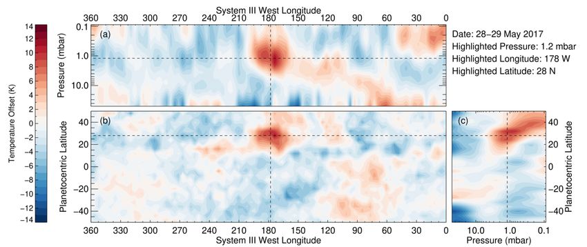
Figure 5: Earth’s equatorial QBO from 1980–2020; figure from NASA/GSFC Data Services (https://acd-
ext.gsfc.nasa.gov/Data services/met/qbo/qbo.html). Radiosonde temperature data were obtained from the Meteorological Service
Singapore Upper Air Observatory and the data have been detrended and the annual cycle has been removed. The 2015–2016 QBO disruption
can be clearly seen (Newman et al., 2016).
9is ordinarily one of the most repeatable phenomena in the meant that the subtropical easterly jet in the winter lower
Earth’s atmosphere, with an oscillation period that has stratosphere was unusually weak; this allowed westward-
varied between 22 and 34 months (Baldwin et al., 2001). In moving Rossby waves to propagate southwards into the
2015–2016, a disruption was observed in the typical QBO equatorial region, and deposit a large flux of westward
pattern for the first time in over sixty years of observa- momentum at 40 mbar.
tions. Osprey et al. (2016) and Newman et al. (2016) show Like the Earth and Jupiter, Saturn also has an oscil-
the QBO disruption in terms of the zonal winds; Figure 5 lation in the equatorial stratosphere. This oscillation is
shows the disruption in terms of the stratospheric temper- known as Saturn’s Semi-Annual Oscillation (SSAO) and it
ature anomalies, allowing it to be directly compared with has a period of 14.7±0.9 years (Orton et al., 2008; Fouchet
Figure 3. Newman et al. (2016) describe the disruption as et al., 2008). Fletcher et al. (2017a) found that in 2011–
an apparent upward displacement of an anomalous west- 2014, the SSAO was disrupted by an intense storm in the
erly wind and the development of easterlies at 40 mbar; northern mid-latitudes. The storm consisted of power-
this has the effect of altering the short-term behavior of the ful convective plumes in the troposphere, and led to the
oscillation, producing an unusually long-lasting 23-month formation of a large, hot, westward-moving vortex in the
eastward phase at 20 mbar, compared to the average 14- stratosphere at 40◦ N (Fletcher et al., 2012). This vortex
month duration (Kumar et al., 2018). In the temperature (known as the ‘beacon’) persisted for over three years, sig-
data shown in Figure 5, this manifests as an upward dis- nificantly longer than the tropospheric storm. At its peak,
placement in the warm branch and the development of a the beacon had a temperature that was 80 K higher than
new cold branch at 40 mbar. the surrounding quiescent regions at 2 mbar. During the
This is morphologically similar to Figure 3, which shows same time period, Fletcher et al. (2017a) showed that the
an upward displacement of the QQO’s descending warm SSAO signature was essentially absent, before resuming in
branch in 2017. As with the 2015–2016 QBO disruption, 2014. As with the Earth’s QBO disruption, Fletcher et al.
this has the effect of altering the short-term behavior of (2017a) attribute the SSAO disruption to an injection of
the QQO, producing an unusually long cold phase at 13.5 westward momentum in the equatorial regions by extrat-
mbar. However, we should note that the QBO disrup- ropical waves; in this case, the waves were thought to be
tion in 2015–2016 was a highly unusual event; the earth’s driven by the hot beacon and/or the underlying storm.
wind patterns and temperatures have been consistently As both the QBO disruption and the SSAO disruption
tracked for over 60 years, providing a vertically-resolved were caused by the propagation of extratropical waves, we
long-term dataset, and Figure 5 shows that this was a used the TEXES zonally-resolved temperatures maps to
unique event within that time period. In contrast, it is search for any unusual behavior that could be associated
unclear whether the QQO disruption shown in Figure 3 is with the 2017 QQO disruption. We found a high-altitude,
an uncommon event, as vertically-resolved measurements mid-latitude thermal anomaly in the May/June 2017 data,
of the QQO have only been made since 2012. 7.8-μm imag- the same observing run in which the disruption was first
ing data have been made since 1980 (Orton et al., 1991; observed; an inspection of the spatially-resolved tempera-
Leovy et al., 1991), but these observations do not provide ture maps from the other observing runs showed that this
vertical resolution and are therefore not able to fully cap- was the largest thermal anomaly observed over the eight
ture the effect of a vertical displacement of the QQO; it year time period.
is possible that some of the variability in the oscillation The May/June 2017 thermal anomaly is shown in Fig-
period observed in the imaging data (Simon-Miller et al., ures 6 and 7. Figure 6 shows three different slices through
2006) is due to a similar type of disruption. the three-dimensional temperature map obtained using
data from May 28–29. The temperature offset is defined
4.3. Potential causes of the 2017 disruption as the temperature relative to the mean zonal tempera-
Based on Figures 3 and 4, we conclude that there was a ture at a given pressure and latitude level. The average
disruption to the QQO pattern in 2017; this disruption retrieved error on the temperature offsets is ∼2 K. Fig-
consisted of an upward displacement of the descending ure 6(a) shows the thermal anomaly as a function of pres-
warm branch, leading to a phase shift in the oscillation. sure and longitude, at a latitude of 28◦ N; 6(b) shows the
Numerical modeling of the observed disruption is beyond thermal anomaly as a function of latitude and longitude,
the scope of this paper and will be a subject for future at a pressure of 1.2 mbar; and 6(c) shows the thermal
study. Instead, we discuss here the causes of similar dis- anomaly as a function of latitude and pressure, at a longi-
ruptions on other planets and present observations of a tude of 178◦ W. In each case, the dashed black lines high-
high-altitude thermal anomaly that may be linked to the light the latitude, longitude and pressure of interest; the
observed disruption. three images intersect at the intersection of the dashed
Barton and McCormack (2017) found that the Earth’s black lines. Figure 7 shows a comparable set of images for
QBO disruption in 2015–2016 was caused by the propa- data obtained on June 5.
gation of Rossby waves from the extratropical Northern Both Figures 6 and 7 show a warm high-altitude double-
Hemisphere. The combination of the timing of the QBO peaked thermal anomaly centered at a latitude of 28◦ N and
relative to the annual cycle and an extreme El Niño event a pressure of 1.2 mbar. This is located in Jupiter’s North
10Figure 6: A warm thermal anomaly, as seen on May 28–29 2017. The three frames show three orthogonal slices through a three-dimensional
retrieved temperature map; these slices are centered on a warm thermal anomaly. The temperature offset is defined as the temperature
relative to the mean zonal temperature at a given pressure and latitude level.
Figure 7: The same thermal anomaly shown in Figure 6, as seen on June 5 2017.
11Temperate Belt, northwards of the planet’s strong pro- matic clearing in Jupiter’s equatorial cloud layer, result-
grade jet at 23◦ N (Porco et al., 2003). By fitting a Gaus- ing in a sharp increase in the 5-μm brightness. The most
sian curve to the retrieved temperatures as a function of recent disturbance described in Antuñano et al. (2018) oc-
longitude, we find that the thermal anomaly moves west- curred in 2006–2007, and they predicted a new equato-
ward with a velocity of 1.5±0.3 degrees/day; at a latitude rial zone disturbance in 2019–2021. Changes in the 5-μm
of 28◦ N, this is equivalent to 19±4 ms-1 . No anomaly was brightness began to be observed in late 2018 (Orton et al.,
present at the same latitude and pressure region during 2019), over a year after the QQO disruption. Finally, we
the January 2017 or February 2018 observing runs. It was consulted the archives of the British Astronomical Associ-
also not observed in July 2017, although full longitudinal ation (BAA1 ), who keep a detailed record of observations
coverage was not obtained on this occasion and the rel- of Jupiter made by amateur astronomers. BAA reports
evant longitudes were not observed (assuming a constant carefully document the outbreak in the North Temperate
velocity of 1.5 degrees/day). Belt in October 2016, but there was no similar outbreak
The correlation between the timing of this thermal observed in spring/summer 2017, despite a large dataset
anomaly and the disruption of the QQO is suggestive of of observations (Rogers, 2017).
a link between these two events. In addition, the thermal While Jupiter’s troposphere exhibits constant activity,
anomaly has some features in common with the strato- the 2017 QQO disruption does not appear to coincide with
spheric ‘beacon’ on Saturn that disrupted the SSAO; this any large global-scale tropospheric upheaval events that
thermal anomaly is also a westward-moving hotspot in the could be seen in visible or infrared observations. It is
stratospheric mid-latitudes. However, the scales of the two possible that a storm could have been present deeper in
hotspots are very different. Saturn’s beacon was 80 K Jupiter’s atmosphere, below the visible cloud deck, but it
warmer than its surroundings and persisted for over three is difficult to see how such a storm could affect strato-
years, while the thermal anomaly we observe here was 13 spheric temperatures without causing a visible plume.
K warmer than its surroundings and persisted for less than Further monitoring of Jupiter’s stratospheric and tropo-
seven months. It is unclear whether a thermal anomaly on spheric temperatures will be required to make further
this smaller scale would have the capacity to influence the progress in understanding the causality of such events in
equatorial temperatures. Jupiter’s atmosphere.
Jupiter’s troposphere undergoes large-scale upheavals
relatively frequently. These events have the ability to dra-
matically change the appearance of the planet by altering 5. Conclusions
the cloud structure (Sánchez-Lavega et al., 2008; Fletcher
et al., 2017b) and would be plausible candidates for driving In this paper, we used high-resolution mid-infrared data
a disruption in the QQO and/or causing localized thermal from TEXES/IRTF to track the evolution of Jupiter’s
anomalies in the stratosphere; rather than causing the dis- quasi-quadrennial oscillation (QQO) over the course of ap-
ruption directly, one possibility is that both the thermal proximately two full cycles (2012–2019). We used a radia-
anomaly and the QQO disruption are the result of a local- tive transfer model to retrieve the zonally-averaged and
ized storm deep in Jupiter’s troposphere. However, there zonally-resolved atmospheric temperatures in the 0.01–30
were no notable planetary scale disturbances during the mbar pressure range. Using the temperature maps ob-
2017–2018 timeframe that we can easily tie to the QQO tained from these retrievals, we come to the following con-
disturbance, despite an extensive search of images from clusions:
different sources.
Sánchez-Lavega et al. (2017) report on a large distur- 1. Between 2012 and 2017, the 13.5-mbar equatorial
bance in Jupiter’s North Temperate Belt in October 2016, temperatures had a smoothly sinusoidal pattern with
consisting of a set of four powerful plumes located at 23◦ N, a period of 4.0±0.2 years and an amplitude of 7±1
that moved eastward with time. However, this activity had K at 13.5 mbar (our region of maximum sensitivity).
ceased by late November 2016, seven months before the During this same time period, the 13.5-mbar temper-
QQO disturbance and the mid-latitude thermal anomaly atures at ±14◦ were in anti-phase with the equatorial
were observed. Wong et al. (2020) present an archive temperatures. This is consistent with previous studies
of high spatial resolution images of Jupiter in the 2016– of the QQO (Orton et al., 1991; Friedson, 1999).
2020 time period; their observations provide good tem- 2. Between 2012 and 2017, the 6.4-mbar and 3.0-mbar
poral coverage in the spring–summer 2017 timeframe and equatorial temperatures also displayed an approxi-
include full longitudinal coverage in the visible from Hub- mately sinuoidal pattern, with a similar period. This
ble’s Wide Field Camera 3 in April 2017, but they note no extension of the QQO up to these lower pressure levels
large convective storm in the northern low or mid latitudes was a new result presented in Cosentino et al. (2017)
beside the one observed in October 2016. Antuñano et al. using the 2012–2016 TEXES data.
(2018) describe a pattern of semi-regular disturbances in
Jupiter’s equatorial zone, occurring with a periodicity of
6–8 or 13–14 years. These disturbances consist of a dra- 1 britastro.org
123. In 2017, there was a disruption to the QQO pattern. Borysow, A., Frommhold, L., 1986. Theoretical collision-induced
This disruption is evident at 3-20 mbar, and appears rototranslational absorption spectra for the outer planets: H2 -
CH4 pairs. The Astrophysical Journal 304, 849–865.
to manifest as an abrupt upward displacement of the Borysow, J., Frommhold, L., Birnbaum, G., 1988. Collison-induced
descending warm branch. This disruption has simi- rototranslational absorption spectra of H2 -He pairs at tempera-
larities to the disruption of the Earth’s QBO in 2015– tures from 40 to 3000 K. The Astrophysical Journal 326, 509–515.
2016. Brown, L.R., Benner, D.C., Champion, J.P., Devi, V.M., Fejard,
L., Gamache, R., Gabard, T., Hilico, J., Lavorel, B., Loete, M.,
4. In May/June 2017, we observed a localized warm ther- et al., 2003. Methane line parameters in HITRAN. Journal of
mal anomaly located at a latitude of 28◦ N and a pres- Quantitative Spectroscopy and Radiative Transfer 82, 219–238.
sure of 1.2 mbar. By comparing observations made ∼1 Cosentino, R.G., Morales-Juberı́as, R., Greathouse, T., Orton, G.,
Johnson, P., Fletcher, L.N., Simon, A., 2017. New observations
week apart, we found that this thermal anomaly was and modeling of Jupiter’s quasi-quadrennial oscillation. Journal
moving westward with a velocity of 19±4 ms-1 of Geophysical Research: Planets 122, 2719–2744.
Drossart, P., Fouchet, T., Crovisier, J., Lellouch, E., Encrenaz, T.,
Based on the timing of the warm thermal anomaly, there Feuchtgruber, H., Champion, J., 1999. Fluorescence in the 3 mi-
is a possibility that it may be related to the QQO disrup- cron bands of methane on Jupiter and Saturn from ISO/SWS
tion that we observe. We note that a hot thermal anomaly observations, in: The Universe as seen by ISO, p. 169.
Dunkerton, T.J., 1997. The role of gravity waves in the quasi-biennial
in Saturn’s mid-latitude stratosphere was linked to a dis- oscillation. Journal of Geophysical Research: Atmospheres 102,
ruption in the SSAO. However, the warm anomaly that 26053–26076.
we observe in Jupiter’s stratosphere is significantly cooler Flasar, F.M., Kunde, V., Achterberg, R., Conrath, B., Simon-Miller,
A., Nixon, C., Gierasch, P., Romani, P., Bézard, B., Irwin, P.,
(∼13 K) and it is unclear whether it would have a signif-
et al., 2004. An intense stratospheric jet on Jupiter. Nature 427,
icant impact on the equatorial regions. One possibility is 132–135.
that both the thermal anomaly and the QQO disruption Fletcher, L.N., Guerlet, S., Orton, G.S., Cosentino, R.G., Fouchet,
are the result of storms deep in Jupiter’s troposphere, al- T., Irwin, P.G., Li, L., Flasar, F.M., Gorius, N., Morales-Juberı́as,
R., 2017a. Disruption of Saturn’s quasi-periodic equatorial oscil-
though no unusual activity was observed during this time lation by the Great Northern Storm. Nature Astronomy 1, 765.
period. Future modelling work is required to better un- Fletcher, L.N., Hesman, B., Achterberg, R., Irwin, P., Bjoraker, G.,
derstand the factors that drive changes to Jupiter’s QQO. Gorius, N., Hurley, J., Sinclair, J., Orton, G., Legarreta, J., et al.,
2012. The origin and evolution of Saturn’s 2011–2012 strato-
spheric vortex. Icarus 221, 560–586.
Acknowledgments Fletcher, L.N., Orton, G., Rogers, J., Giles, R., Payne, A., Irwin, P.,
Vedovato, M., 2017b. Moist convection and the 2010–2011 revival
of Jupiter’s South Equatorial Belt. Icarus 286, 94–117.
This research was primarily funded by NASA Planetary
Fouchet, T., Guerlet, S., Strobel, D., Simon-Miller, A., Bézard, B.,
Astronomy (PAST) grant NNX14AG34G. GSO was sup- Flasar, F., 2008. An equatorial oscillation in Saturn’s middle at-
ported by funds from NASA distributed to the Jet Propul- mosphere. Nature 453, 200.
sion Laboratory, California Institute of Technology. This Friedson, A.J., 1999. New observations and modelling of a QBO-like
oscillation in Jupiter’s stratosphere. Icarus 137, 34–55.
work was based on data obtained with the NASA Infrared Greathouse, T.K., Lacy, J.H., Bézard, B., Moses, J.I., Griffith, C.A.,
Telescope Facility, which is operated by the University of Richter, M.J., 2005. Meridional variations of temperature, C2 H2
Hawaii under a contract with the National Aeronautics and C2 H6 abundances in Saturn’s stratosphere at southern sum-
and Space Administration. The authors would like to ac- mer solstice. Icarus 177, 18–31.
Greathouse, T.K., Richter, M., Lacy, J., Moses, J., Orton, G., En-
knowledge the contributions of many observing collabora- crenaz, T., Hammel, H., Jaffe, D., 2011. A spatially resolved high
tors and NASA/IRTF staff. The authors would also like spectral resolution study of Neptune’s stratosphere. Icarus 214,
to thank the two anonymous reviewers whose comments 606–621.
helped improve and clarify this manuscript. Kumar, K.K., Mathew, S.S., Subrahmanyam, K., 2018. Anoma-
lous tropical planetary wave activity during 2015/2016 quasi bi-
ennial oscillation disruption. Journal of Atmospheric and Solar-
Terrestrial Physics 167, 184–189.
References Lacy, J., Richter, M., Greathouse, T., Jaffe, D., Zhu, Q., 2002.
TEXES: A sensitive high-resolution grating spectrograph for the
References mid-infrared. Publications of the Astronomical Society of the Pa-
cific 114, 153–168.
Allen, R.J., Sherwood, S.C., 2007. Utility of radiosonde wind data Leovy, C.B., Friedson, A.J., Orton, G.S., 1991. The quasiquadrennial
in representing climatological variations of tropospheric tempera- oscillation of Jupiter’s equatorial stratosphere. Nature 354, 380.
ture and baroclinicity in the western tropical Pacific. Journal of Li, X., Read, P., 2000. A mechanistic model of the quasi-quadrennial
Climate 20, 5229–5243. oscillation in Jupiter’s stratosphere. Planetary and Space Science
Antuñano, A., Fletcher, L.N., Orton, G.S., Melin, H., Rogers, J.H., 48, 637–669.
Harrington, J., Donnelly, P.T., Rowe-Gurney, N., Blake, J.S., Margolis, J.S., 1993. Measurement of hydrogen-broadened methane
2018. Infrared characterization of Jupiter’s equatorial disturbance lines in the ν4 band at 296 and 200 K. Journal of Quantitative
cycle. Geophysical Research Letters 45, 10987–10995. Spectroscopy and Radiative Transfer 50, 431–441.
Baldwin, M., Gray, L., Dunkerton, T., Hamilton, K., Haynes, P., Moses, J., Fouchet, T., Bézard, B., Gladstone, G., Lellouch, E.,
Randel, W., Holton, J., Alexander, M., Hirota, I., Horinouchi, T., Feuchtgruber, H., 2005. Photochemistry and diffusion in Jupiter’s
et al., 2001. The quasi-biennial oscillation. Reviews of Geophysics stratosphere: constraints from ISO observations and comparisons
39, 179–229. with other giant planets. Journal of Geophysical Research: Plan-
Barton, C., McCormack, J., 2017. Origin of the 2016 QBO disrup- ets 110.
tion and its relationship to extreme El Niño events. Geophysical Naujokat, B., 1986. An update of the observed quasi-biennial oscil-
Research Letters 44, 11150–11157.
13lation of the stratospheric winds over the tropics. Journal of the
Atmospheric Sciences 43, 1873–1877.
Newman, P., Coy, L., Pawson, S., Lait, L., 2016. The anomalous
change in the QBO in 2015–2016. Geophysical Research Letters
43, 8791–8797.
Orton, G., Antuñano, A., Fletcher, L., Sinclair, J., Momary, T.,
Chowdhury, N., Melin, H., Stallard, T., Rathbun, J., Bjoraker, G.,
et al., 2019. Juno and Juno-supporting observations of Jupiter’s
2018-2019 equatorial zone disturbance, in: EPSC Abstracts.
Orton, G.S., Friedson, A.J., Baines, K.H., Martin, T.Z., West, R.A.,
Caldwell, J., Hammel, H.B., Bergstralh, J.T., Malcom, M.E.,
Golisch, W.F., et al., 1991. Thermal maps of Jupiter: spatial
organization and time dependence of stratospheric temperatures,
1980 to 1990. Science 252, 537–542.
Orton, G.S., Gustafsson, M., Burgdorf, M., Meadows, V., 2007. Re-
vised ab initio models for H2 -H2 collision-induced absorption at
low temperatures. Icarus 189, 544–549.
Orton, G.S., Yanamandra-Fisher, P.A., Fisher, B.M., Friedson, A.J.,
Parrish, P.D., Nelson, J.F., Bauermeister, A.S., Fletcher, L.,
Gezari, D.Y., Varosi, F., et al., 2008. Semi-annual oscillations
in Saturn’s low-latitude stratospheric temperatures. Nature 453,
196.
Osprey, S.M., Butchart, N., Knight, J.R., Scaife, A.A., Hamilton, K.,
Anstey, J.A., Schenzinger, V., Zhang, C., 2016. An unexpected
disruption of the atmospheric quasi-biennial oscillation. Science
353, 1424–1427.
Pascoe, C.L., Gray, L.J., Crooks, S.A., Juckes, M.N., Baldwin, M.P.,
2005. The quasi-biennial oscillation: Analysis using ERA-40 data.
Journal of Geophysical Research: Atmospheres 110.
Porco, C.C., West, R.A., McEwen, A., Del Genio, A.D., Ingersoll,
A.P., Thomas, P., Squyres, S., Dones, L., Murray, C.D., John-
son, T.V., et al., 2003. Cassini imaging of Jupiter’s atmosphere,
satellites, and rings. Science 299, 1541–1547.
Rodgers, C.D., 2000. Inverse Methods for Atmospheric Sounding:
Theory and Practice. World Scientific.
Rogers, J., 2017. Jupiter in 2016-2017. British Astronomical Asso-
ciation URL: https://britastro.org/node/8103.
Rothman, L.S., Jacquemart, D., Barbe, A., Benner, D.C., Birk, M.,
Brown, L., Carleer, M., Chackerian, C., Chance, K., Coudert, L.,
et al., 2005. The HITRAN 2004 molecular spectroscopic database.
Journal of Quantitative Spectroscopy and Radiative Transfer 96,
139–204.
Sánchez-Lavega, A., Orton, G., Hueso, R., Garcı́a-Melendo, E.,
Pérez-Hoyos, S., Simon-Miller, A., Rojas, J., Gómez, J.,
Yanamandra-Fisher, P., Fletcher, L., et al., 2008. Depth of a
strong jovian jet from a planetary-scale disturbance driven by
storms. Nature 451, 437.
Sánchez-Lavega, A., Rogers, J.H., Orton, G., Garcı́a-Melendo, E.,
Legarreta, J., Colas, F., Dauvergne, J., Hueso, R., Rojas, J.F.,
Pérez-Hoyos, S., et al., 2017. A planetary-scale disturbance in the
most intense jovian atmospheric jet from JunoCam and ground-
based observations. Geophysical Research Letters 44, 4679–4686.
Simon-Miller, A.A., Conrath, B.J., Gierasch, P.J., Orton, G.S.,
Achterberg, R.K., Flasar, F.M., Fisher, B.M., 2006. Jupiter’s
atmospheric temperatures: from Voyager IRIS to Cassini CIRS.
Icarus 180, 98–112.
Wong, M.H., Simon, A.A., Tollefson, J.W., de Pater, I., Barnett,
M.N., Hsu, A.I., Stephens, A.W., Orton, G.S., Fleming, S.W.,
Goullaud, C., et al., 2020. High-resolution UV/Optical/IR Imag-
ing of Jupiter in 2016–2019. The Astrophysical Journal Supple-
ment Series 247, 58.
14You can also read