Where did they not go? Considerations for generating pseudo-absences for telemetrybased habitat models
←
→
Page content transcription
If your browser does not render page correctly, please read the page content below
Hazen et al. Movement Ecology        (2021) 9:5
https://doi.org/10.1186/s40462-021-00240-2

 RESEARCH                                                                                                                                          Open Access

Where did they not go? Considerations for
generating pseudo-absences for telemetry-
based habitat models
Elliott L. Hazen1,2,3* , Briana Abrahms1,4, Stephanie Brodie1,3, Gemma Carroll1,3, Heather Welch1,3 and
Steven J. Bograd1,3

  Abstract
  Background: Habitat suitability models give insight into the ecological drivers of species distributions and are
  increasingly common in management and conservation planning. Telemetry data can be used in habitat models to
  describe where animals were present, however this requires the use of presence-only modeling approaches or the
  generation of ‘pseudo-absences’ to simulate locations where animals did not go. To highlight considerations for
  generating pseudo-absences for telemetry-based habitat models, we explored how different methods of pseudo-
  absence generation affect model performance across species’ movement strategies, model types, and environments.
  Methods: We built habitat models for marine and terrestrial case studies, Northeast Pacific blue whales (Balaenoptera
  musculus) and African elephants (Loxodonta africana). We tested four pseudo-absence generation methods commonly
  used in telemetry-based habitat models: (1) background sampling; (2) sampling within a buffer zone around presence
  locations; (3) correlated random walks beginning at the tag release location; (4) reverse correlated random walks
  beginning at the last tag location. Habitat models were built using generalised linear mixed models, generalised
  additive mixed models, and boosted regression trees.
  Results: We found that the separation in environmental niche space between presences and pseudo-absences was
  the single most important driver of model explanatory power and predictive skill. This result was consistent across
  marine and terrestrial habitats, two species with vastly different movement syndromes, and three different model
  types. The best-performing pseudo-absence method depended on which created the greatest environmental
  separation: background sampling for blue whales and reverse correlated random walks for elephants. However, despite
  the fact that models with greater environmental separation performed better according to traditional predictive skill
  metrics, they did not always produce biologically realistic spatial predictions relative to known distributions.
  Conclusions: Habitat model performance may be positively biased in cases where pseudo-absences are sampled from
  environments that are dissimilar to presences. This emphasizes the need to carefully consider spatial extent of the
  sampling domain and environmental heterogeneity of pseudo-absence samples when developing habitat models, and
  highlights the importance of scrutinizing spatial predictions to ensure that habitat models are biologically realistic and
  fit for modeling objectives.

* Correspondence: Elliott.hazen@noaa.gov
1
 NOAA Southwest Fisheries Science Center, Environmental Research Division,
Monterey, CA, USA
2
 Department of Ecology and Evolutionary Biology, University of California
Santa Cruz, Santa Cruz, CA, USA
Full list of author information is available at the end of the article

                                       © The Author(s). 2021 Open Access This article is licensed under a Creative Commons Attribution 4.0 International License,
                                       which permits use, sharing, adaptation, distribution and reproduction in any medium or format, as long as you give
                                       appropriate credit to the original author(s) and the source, provide a link to the Creative Commons licence, and indicate if
                                       changes were made. The images or other third party material in this article are included in the article's Creative Commons
                                       licence, unless indicated otherwise in a credit line to the material. If material is not included in the article's Creative Commons
                                       licence and your intended use is not permitted by statutory regulation or exceeds the permitted use, you will need to obtain
                                       permission directly from the copyright holder. To view a copy of this licence, visit http://creativecommons.org/licenses/by/4.0/.
                                       The Creative Commons Public Domain Dedication waiver (http://creativecommons.org/publicdomain/zero/1.0/) applies to the
                                       data made available in this article, unless otherwise stated in a credit line to the data.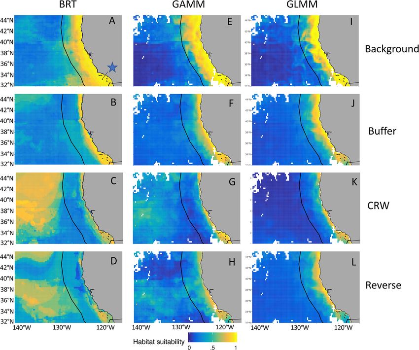
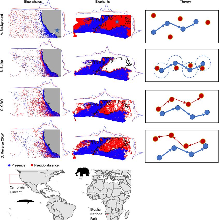
Hazen et al. Movement Ecology   (2021) 9:5                                                                    Page 2 of 13

Background                                                       In order to highlight key considerations for generating
Animal telemetry has revolutionized our understanding         pseudo-absences for habitat models built from telemetry
of animal movement and habitat use in both marine and         data, the effects and biases of pseudo-absence generation
terrestrial environments [29, 35]. Telemetry data have        methods need to be explored across species’ movement
allowed for the exploration of behavioural and environ-       strategies, model types, and environments. Here we
mental drivers of animal space use, habitat selection,        examine pseudo-absence generation methods using two
and migration [4, 39, 43, 49], and enabled the identifica-    mobile megafauna, the blue whale (Balaenoptera muscu-
tion of important biological hotspots to inform conser-       lus) and African elephant (Loxodonta africana). These
vation and management [14, 32, 55]. Animal telemetry          two species forage near the base of the food web, yet in-
data can also be used as inputs to habitat models (also       habit completely different physical environments and
known as ‘species distribution models’), to predict pat-      employ different movement strategies [2, 8, 61]. In the
terns of distribution or resource selection across space      Northeast Pacific, blue whales undertake basin-scale mi-
and time based on a species’ preference for particular        grations from breeding to foraging grounds, while in
characteristics of the environment [25]. However, a fun-      Etosha National Park, Namibia, elephants move nomad-
damental challenge of using telemetry data in habitat         ically within the park boundaries. For each species, we
models is that they are presence-only, and thus cannot        compare the effects of four different pseudo-absence
be used to infer environmental drivers in areas where         generation techniques (background sampling, buffer
animals were absent. To address this, a variety of tech-      sampling, CRW and reverse CRW) on habitat model
niques exist to generate data representing where animals      performance. We compare results across three model
could have gone but did not go (i.e. ‘pseudo-absences’,       types commonly applied to telemetry data (generalised
e.g. [9]). However, the relative performances of different    linear mixed models, generalised additive mixed models
pseudo-absence generation methods have not yet been           and boosted regression trees) to test if the relative per-
assessed for telemetry-based habitat models. Further-         formance of different pseudo-absence generation
more, the literature lacks an evaluation of the relative      methods was robust across different model types.
utility of pseudo-absence methods between marine and
terrestrial systems, where differences in the scales of       Methods
habitat heterogeneity may influence model outcomes.           Species data
  Approaches for generating pseudo-absences range             We explored two previously published mega-vertebrate
from simple (e.g., background sampling, [46, 54]) to          tracking datasets for Northeast Pacific blue whales and
complex [e.g., biased sampling, [9, 41]]. Background          African elephants (Fig. 1). The blue whale data con-
sampling is the most commonly used approach, which            tained 10,664 daily locations in the eastern North
involves randomly sampling the entire study area or           Pacific, representing 104 ARGOS-tracked blue whales
habitat extent to produce absences that represent a           tracked between 1998 and 2009. This dataset has been
broad range of characteristics [37, 38, 46]. While back-      studied extensively to identify critical habitat [36],
ground sampling is the backbone of presence-only mod-         understand patterns and drivers of migration [2, 8], and
eling techniques such as Maxent [54], it does not             guide spatial management strategies [4, 30]. In this
consider how animals actually move through space and          study, we examined foraging habitat selection by blue
treats all areas and habitats as being equally accessible.    whales when resident in the central California Current
To address this issue, approaches that explicitly incorp-     System (CCS; 2,240,000 km2), excluding migratory be-
orate information on animal movement have been devel-         havior through Mexican waters and presumed breeding
oped, such as buffer sampling (analogous to ‘step             behavior in the southern end of their range. The ele-
selection’ [7, 19, 60]. This approach treats habitat selec-   phant dataset contained 40,273 locations taken every 6 h
tion as a series of step-by-step decisions, with pseudo-      from 14 GPS-collared elephants in Etosha National Park,
absences randomly sampled within a predetermined              Namibia (EtNP; 22,900 km2) between 2008 and 2014.
step-length from each presence location. A third ap-          These data have previously been used to explore animal
proach is to create pseudo-absences that have the same        movement syndromes [3] and drivers of habitat use [61].
autocorrelation structure as actual tracks using corre-
lated random walks (CRWs) [1, 30, 31, 42, 67]. CRWs           Environmental data
recreate movement patterns using sampled step-lengths         We selected six out of twelve potential environmental
and turn angles from interpolated animal tracks, in order     variables for blue whales that have previously been
to realistically simulate the movement characteristics of     shown to be important drivers of habitat use during mi-
study species. CRWs can also be generated in reverse          gration and foraging [4, 30, 52]: sea surface temperature,
(reverse CRWs) to control for biases generated by non-        the spatial variability of sea surface temperature (an
random animal tagging locations [53].                         index of frontal activity), sea level anomaly, chlorophyll-
Hazen et al. Movement Ecology          (2021) 9:5                                                                                          Page 3 of 13

 Fig. 1 Presence data (blue points) and pseudo-absence data (red points) for the four pseudo-absence generation techniques a background, b
 buffer, c Correlated Random Walks (CRWs), d reverse CRW for blue whales (left), elephants (middle), and in theory (right). White represents areas
 unvisited by tagged individuals or simulated pseudo-absences. Density by latitude (top of panel) and longitude (right side of panel) highlights
 the difference in pseudo-absence sampling approach (red) from observed habitat using tracking data (blue). The Southern California Bight (top
 left) and salt pans (middle left) are indicated with blue stars. Study domains of the California Current, U.S. and Etosha National Park, Namibia are
 shown in the bottom two panels. In the right-most panels, the theory behind calculation of pseudo-absences for each approach is shown with
 blue being actual positions and red being simulated positions

a, oxygen concentration at 100 m depth, and bathymetry                        nearest water source. The two study systems, the CCS
(Table S1). For elephants, we selected three variables                        and EtNP, have vastly different patterns of environmen-
that have been shown to most strongly influence ele-                          tal dynamism. The CCS has strong seasonal upwelling
phant movement in the study area (Table S1, [61]): dis-                       driving cool, productive nearshore waters [15], with off-
tance to the nearest road, multiannual mean normalized                        shore waters characterized by ephemeral features like
difference vegetation index (NDVI), and distance to the                       fronts and eddies that can shift at daily to weekly
Hazen et al. Movement Ecology   (2021) 9:5                                                                       Page 4 of 13

timescales [20]. In contrast, EtNP experiences more             measured movement parameters such as distance trav-
gradual seasonal variation in temperature and rainfall          eled and turning angle between consecutive locations
[61]. Accordingly, the environmental variables selected         [42]. CRWs have been implemented particularly when
for modelling mirror this dynamism: dynamic variables           animals are wide ranging and can access areas far from
for the CCS were acquired at a daily or monthly reso-           the original tagging location [67]. In theory, CRWs offer
lution, whereas EtNP variables were either static or            the ability to create absences that best reflect the spatial
long-term averages (in the case of NDVI).                       and temporal auto-correlation of the actual tracks. Fur-
                                                                ther, when there are implicit drivers of directionality or
Pseudo-absence types                                            seasonality (e.g. movement away from competing col-
We compared four methods of pseudo-absence gener-               onies, or migration through less desirable habitat to
ation that represent different assumptions about where          reach more favorable habitat), entire CRW tracks can be
animals could be distributed relative to observed tracks:       selected that appropriately recreate important features of
‘background sampling’, where random locations are sam-          original tracks, such as the maximum displacement, or
pled across the entire domain; ‘buffer sampling’, where         the mean angle of travel [30, 63]. Reverse CRWs have
random locations are sampled within a certain distance          been introduced to address the issue of biases in tagging
from each presence location; and ‘correlated random             locations, recreating movement from the last known lo-
walks’ (CRW) and ‘reverse CRWs’, where tracks are sim-          cation and simulating backwards in time to the original
ulated from given start or end points respectively, based       tagging date [53].
on observed step lengths and turn angles. We outline
each method below, and illustrate key concepts in Fig. 1.       Pseudo-absence generation
  Background sampling is designed to capture the full           We used a common sampling extent for all generation
range of conditions under which species could be found,         methods for each species based on the maximum extent
assuming they were distributed randomly across the en-          of their tracks: for blue whales, a bounding box from 32°
vironment. Habitat models are then used to contrast             to 45° N and − 140° to − 115° W within the CCS; and for
characteristics of preferred habitat where species are          elephants the fenced boundary of EtNP (Fig. 1). For each
more likely to be observed, with this completely random         pseudo-absence method, we generated a 1:1 ratio of
distribution [21]. This approach is adapted from system-        pseudo-absences to presences to maintain consistency
atic survey design ([37] and references therein), where         across models.
individual presences are not assumed to be autocorre-             For background sampling, pseudo-absences were
lated [59]. Thus, even when applied to tracking data            drawn randomly from within the domain for each spe-
where each presence location depends on the one pre-            cies. For buffer sampling, we used the mode step length
ceding it, background sampling of pseudoabsences in-            to create a radius of 100 km (whales) and 10 km (ele-
corporates no information or assumptions regarding              phants) around each presence point, and randomly sam-
characteristics of animal movement, such as distance            pled one absence within each buffer zone. For CRWs,
traveled or direction of movement.                              we randomly sampled a paired distance and turn angle
  Buffer sampling for habitat modeling was originally           from the observed distributions. Points were generated
used to minimize pseudo-absence overlap with pres-              consecutively, starting from the locations where animals
ences, by sampling points outside a certain radius              were tagged, until the number of pseudo-absences
around each presence [33]. However, more recent ap-             equaled the number of presences. The reverse CRW
proaches use buffers to restrict the sampling domain to         used the same approach but instead moved backwards
areas accessible by the animal, by sampling from within         in time from the last recorded position of the tag.
a given radius around a presence [10, 24]. For tracking
data, buffer size has been determined based on the mean         Habitat modeling
or median step-length (e.g. distance traveled between           We selected three commonly used statistical correlative
two positions over a set time interval), irrespective of        models to test how model type influenced the relative
direction [34]. Resource selection functions use buffer         performance of the pseudo-absence generation methods.
sampling at each step to estimate the relative probability      We selected generalised linear mixed models (GLMMs),
of selecting a specific parcel of habitat, relative to others   which are parametric and estimate linear species-
that were equally accessible at that movement step [46].        environment relationships; generalised additive mixed
  CRWs and reverse CRWs sample the paired distribu-             models (GAMMs) which are semi-parametric and use
tion of distance and turn angle from the empirical move-        smoothers to represent non-linear species-environment
ment distributions in order to simulate realistic tracks        relationships; and boosted regression trees (BRTs) which
(e.g. [1, 30]). CRWs have been used to create potential         are non-parametric and use boosting to determine opti-
trajectories that animals could have taken based on             mal partitioning of variance. For both GLMMs and
Hazen et al. Movement Ecology (2021) 9:5 Page 5 of 13
GAMMs, we used the gamm function in the ‘mgcv’ R using expert knowledge. Specifically, we considered
package [64] and included individual tag identification as spatial predictions biologically realistic for blue whales if
a random effect. For GAMMs, we used a thin-plate they predicted inshore habitat along the coast and repro-
spline smoother with knots set to 5 per variable. BRTs duced the known blue whale hotspot in the Southern
were fit using the gbm.fixed function in the ‘dismo’ R California Bight during summer months [12, 18, 36]; we
package [23] with a learning rate of 0.005, a bag fraction considered spatial predictions biologically realistic for el-
of 0.75, tree complexity of 5, and 2000 trees (following ephants if they avoided predictions in the large salt pan
[26]). in the northeast corner of EtNP and preferred areas
closer to roads, water, and fences [61]. We also quanti-
Model performance fied the ability of models to capture where blue whales
We evaluated model performance holistically across and elephants are present and putatively absent by cal-
three dimensions: explanatory power, predictive skill, culating mean predicted values at known presences and
and biological realism. Explanatory power indicates a pseudo-absences, respectively.
model’s ability to explain the variability in a given data-
set, and was evaluated using % explained deviance (R2). Results
Predictive skill indicates a model’s ability to correctly Spatial and environmental separation of pseudo-absences
predict species presence or absence on novel data, and and presences
was evaluated with Area Under the Receiver Operating Blue whale presences were clustered adjacent to the
Characteristic Curve (AUC) and True Skill Statistic California coastline, with highest densities in the South-
(TSS, [5]). As independent validation data do not exist at ern California Bight (Fig. 1). Elephant presences were
the scale of the original data, we tested predictive skill clustered in the southern portion of EtNP, and no pres-
using three cross-validation approaches: the first used ences were located within the large salt pan in the
100% of the data for both model training and testing. northeast corner of the park (Fig. 1). There was similar
The second used randomly subsampled 75% of the data spatial separation between pseudo-absences and pres-
to train models, with the remaining 25% used to test ences across the four generation methods for both spe-
models. Third, we also trained models on 11 of 12 cies (Fig. 1). Background sampling - which randomly
months, and withheld a single month (twelve times) for sampled pseudo-absences across the study area - re-
testing for the dynamic blue whale models. As the ter- sulted in the greatest spatial contrast between pseudo-
restrial predictors for elephants were static or climato- absences and presences, with pseudo-absences sampled
logical averages, we were unable to test a temporal in offshore regions of the CCS, and in the salt pan and
leave-one-out approach. We present the 100% training northern extent of EtNP (Fig. 1). Buffer sampling -
and testing results so that inferences were consistent which sampled pseudo-absences within 100 km and 10
across validation approaches. km of blue whale and elephant presences, respectively,
Previous work has identified that habitat model per- resulted in the lowest spatial contrast between pseudo-
formance will increase as environmental dissimilarity be- absences and presences, while CRW and reverse CRW
tween presences and absences increases [45]. We resulted in intermediate spatial contrast (Fig. 1).
explored this phenomenon by using density plots to The separation of environmental variables between
qualitatively evaluate the environmental dissimilarity be- presence and pseudo-absence locations were similar to
tween presences and pseudo-absences generated by the the spatial contrasts among pseudo-absence generation
four methods. Additionally, we quantified the statistical methods (Fig. 2). For blue whales, background sampling
independence of the environmental niches of the pres- had the greatest environmental separation between pres-
ences and pseudo-absences for each variable and species ences and pseudo-absences for all variables, largely due
using Bhattacharayya’s coefficient [13]. To determine the to the preference of tracked animals for the nearshore
effect of environmental dissimilarity on model perform- 200 m depth contour and the strong onshore-offshore
ance, we used linear regression to test relationships be- environmental gradients that were sampled by the
tween Bhattacharyya’s coefficient and model predictive pseudo-absences (Fig. 2a-d). For example, sea surface
skill (AUC) for the three most important predictor vari- temperature had a single peak at 28 °C for background
ables for each species. sampling, compared to double peaks around 28 °C and
Finally, [62] recommended supplementing evaluations 16 °C in the presence data, CRW, reverse CRW, and buf-
of model performance with evaluations of biological fer sampling (Fig. 2a). All pseudo-absence methods sam-
realism based on expert opinion and published litera- pled deeper, more oxygenated waters with lower
ture. Following this advice, we qualitatively evaluated the chlorophyll concentrations compared to the blue whale
ability of the models to predict realistic patterns of spe- presences (Fig. 2b-d). The elephants showed less envir-
cies distributions by assessing spatial prediction maps onmental separation between pseudo-absences andHazen et al. Movement Ecology (2021) 9:5 Page 6 of 13
Fig. 2 Degree of environmental separation for key predictor variables between presences (black line) and each pseudo-absence generation
technique (colors) for blue whales (a-d), and elephants (e-g). Grey shading represents overlap across all techniques
presences compared to blue whales, and fewer differ- GLMMs in terms of explanatory power and predictive
ences in separation among pseudo-absence methods skill for both species.
(Fig. 2e-g). For elephants, buffer sampling resulted in the Environmental similarity between presences and
greatest environmental overlap between pseudo- pseudo-absences (Bhattacharyya’s coefficient) had a sig-
absences and presences for the three predictor variables, nificant negative relationship (p < 0.05) with model pre-
whereas reverse CRW sampling had the lowest overlap dictive skill (AUC) for each model type and species
with presences. Pseudo-absence methods generally sam- (Fig. 3). That is, as the environments sampled by
pled areas that were further from roads and water, and pseudo-absences became more similar to presence loca-
with lower NDVI values compared to where elephants tions, model performance decreased. This pattern was
were present (Fig. 2e-g). For both species, habitat model also reflected in the relationship between Bhattacharyya’s
response curves highlighted how unique the environ- coefficient and both TSS and R2 values (Table 1). The
mental data range of background sampling was com- lowest Bhattacharyya’s coefficient (highest environmen-
pared to the other pseudo-absence methods (Fig. S1). tal separation) was found in blue whale background
sampling, which also had the highest R2, AUC, and TSS
values across all models and both species. Conversely,
Model performance the highest Bhattacharyya’s coefficient (lowest environ-
Blue whale model performance was strongly driven by mental separation) was found in the elephant buffer
pseudo-absence type, with models built using back- sampling, which also had the lowest R2, AUC, and TSS
ground sampling having the best explanatory power, values across all models and species (Table 1, Tables S1,
predictive skill, and ability to capture where blue whales S2). These results provide evidence that model explana-
are present (Table 1). CRWs were best able to capture tory power and predictive skill is strongly related to en-
where blue whales were absent (mean prediction at vironmental separation between presences and absences,
pseudo-absences). In contrast, elephant model perform- regardless of species or habitat model type.
ance was predominantly influenced by model type, with Spatial predictions of species distributions showed di-
BRTs having the best explanatory power, predictive skill, vergent results across pseudo-absence generations
and ability to capture where elephants were absent re- methods and model types. For blue whales, background
gardless of pseudo-absence type. This pattern of BRTs sampling predicted more uniformly suitable habitat on
performing best was also apparent in blue whales, but to the continental shelf, whereas other pseudo-absence
a lesser extent due to the large effect of pseudo-absence methods predicted higher inshore use. CRWs and re-
type (Table 1). Following BRTs, GAMMs outperformed verse CRWs were best able to reproduce the known blueHazen et al. Movement Ecology (2021) 9:5 Page 7 of 13 Table 1 Summary of model predictive skill statistics (R2, AUC, TSS) for blue whale and elephant habitat models, each model type, and each pseudo-absence generation technique. Biological realism was assessed using the predictions at simulated absences and true presences, with visual realism assessed by the full suite of authors based on skill within the Southern California Bight (blue whales) and Etosha salt pan (elephants). Figure panel is also included for Fig. 4 (blue whales) and 5 (elephants) to aid cross- referencing. The best performing model using 100% test and training is shown in red with the worst shown in blue. For R2, AUC, TSS, and Predictions at presences, high values indicate better performance. For Predictions at pseudo-absence, values closer to 0 indicate better performance. Bold values are the top 4 performing models in each category, with blue backgrounds representing the best performing in that category and red representing worse whale hotspot in the Southern California Bight during GLMMs and GAMMs predicted smoother and more summer months [12, 18, 36]. In general, there was more homogeneous distributions (Fig. 5). consistency in spatial predictions among model types than among pseudo-absence generation methods (Fig. 4). For Discussion elephants, spatial differences among both pseudo-absence A critical component of habitat modeling for presence- methods and model types were minimal, with all (except only data like animal telemetry is selecting pseudo- GAMM with buffer) reproducing low habitat selection in- absence points that provide insight into how habitat se- side the large salt pan in the northeast of the park (Fig. 5). lected by animals differs from the range of available The BRT model with highest predictive skill was reverse habitat [9]. Here we explored the performance of CRW, while background sampling was able to highlight pseudo-absence generation techniques across species, areas of low habitat preference in the northern extent of study systems, and model types to help inform best the EtNP that matched patterns in the tracking data to a practices for telemetry-based habitat modeling. We greater degree than the other sampling methods and found that the environmental separation between pres- model types (Fig. 5). Elephant BRTs captured fine-scale ences and pseudo-absences was an important driver of patterns of habitat use across pseudo-absence types, while model explanatory power and predictive skill - a result
Hazen et al. Movement Ecology        (2021) 9:5                                                                                    Page 8 of 13

 Fig. 3 Relationship between model predictive skill (AUC; Area Under the Receiver Operating Characteristic Curve) and environmental separation
 between presences and pseudo-absences (Bhattacharyya’s coefficient) for blue whales (upper) and elephants (lower). Bhattacharyya’s coefficient
 was calculated for key environmental covariates (symbols). Sub-panels for each model type (BRT, GAMM, GLMM) are shown, with colors indicating
 pseudo-absence generation technique. The lines represent linear regression between the AUC value and the Bhattacharyya’s coefficient
 independent of pseudo-absence type and variable

that held true across marine and terrestrial habitats, two                within the species’ domain and background sampling
species with different movement syndromes (migratory                      from outside the species’ domain to understand habitat
vs. nomadic), and three different model types. However,                   use. Thus the separation between environmental condi-
greater environmental separation between presences and                    tions in the two sampling extents likely dominates any
pseudo-absences did not necessarily lead to greater bio-                  difference between pseudo-absence approach. Sampling
logical realism in spatial predictions, highlighting the im-              across broad spatial and environmental gradients can be
portance of using multiple inferences to evaluate model                   useful for identifying patterns of presence and absence
performance. Model performance metrics may be posi-                       and result in increased model performance, but may not
tively biased in cases where pseudo-absences are sam-                     be the most appropriate approach for understanding
pled from dissimilar habitats relative to those used by                   finer scale patterns of movement and habitat selection,
the study species, without a concurrent increase in the                   highlighting the need to identify ecological questions
model’s ability to make accurate predictions of habitat                   and applications prior to modeling.
use. This emphasizes the need to carefully consider the                     The four pseudo-absence methods differed in their
spatial extent of the sampling domain and environmen-                     ability to describe patterns in elephant and blue whale
tal separation between presences and sampled pseudo-                      distributions, including correctly differentiating areas
absences when developing habitat models.                                  where species were probably present from areas where
   Previous studies have demonstrated that model per-                     they were probably absent (e.g. offshore CCS, and in the
formance is influenced by study area extent and the pro-                  Etosha salt pan). We assessed biological realism of our
portion of this extent occupied by species, such that                     spatial predictions (Figs. 4 and 5) and found that the
species that occupy small extents of a large study area                   most biologically realistic models were not always those
are better predicted than species that occupy large ex-                   that performed best according to traditional model per-
tents of small study areas [44, 45, 62]. Separation in en-                formance metrics. For example, blue whale background
vironmental niche space may dominate any differences                      sampling had the highest predictive performance, but
between pseudo-absence generation approaches. For ex-                     failed to identify the gradient between off-shelf absence
ample, [51] found CRWs were less successful than back-                    and near-shore suitability where blue whales frequently
ground sampling. However, the study used CRWs only                        occur. Background sampling tended to overestimate
Hazen et al. Movement Ecology         (2021) 9:5                                                                                          Page 9 of 13

 Fig. 4 Effect of pseudo-absence generation type for BRT (a-d, four panels on left), GAMM (e-h), and GLMM models (i-l) and model type using
 background sampling (a, e, i - top three panels), buffer sampling (b, f, j), CRW sampling (c, g, k), and reverse CRW sampling (d, h, l) on blue
 whale model predictions for a given day, August 1st, 2006. Yellow indicates high habitat suitability while blue is low habitat suitability. GLMMs
 and GAMMs have white pixels where there were missing predictor variables (e.g. due to cloud cover) for the day. The blue star in panel A is
 pointing to the Southern California Bight

suitable habitat, and was therefore the most inaccurate                      where modellers should decide a priori on a model’s
at capturing areas where whales were absent (Table 1).                       purpose and whether the ultimate goal is to better pre-
In comparison, CRW sampling was more biologically                            dict species presence or absence (e.g. [28]. We advise
realistic and better at capturing blue whale absence                         caution when comparing model performance across
within the CCS domain despite this sampling approach                         multiple studies that may be driven by different manage-
resulting in models with poorer predictive performance                       ment goals or that use different underlying data, model-
and out of sample testing. Boosted regression tree                           ing types, or pseudo-absence generation approaches. For
models based on CRW and reverse CRW had anomal-                              example, a blue whale habitat modeling application that
ously high offshore habitat predictions where blue                           aims to conservatively identify all areas where whales
whales were rarely present even with strong realism                          might be present in order to afford them maximum
nearshore, indicating these models would not be a good                       spatial protection could benefit from using the back-
candidate for extrapolation [66].                                            ground method, whereas an application that seeks to
  The tradeoff between model skill and biological real-                      identify areas where whales are most likely not in direct
ism has practical implications for habitat modeling,                         contact with human activities outside areas of core
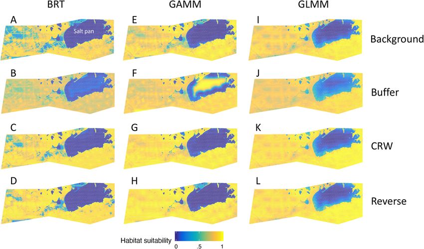
Hazen et al. Movement Ecology         (2021) 9:5                                                                                       Page 10 of 13

 Fig. 5 Effect of pseudo-absence generation type for elephants for BRT (a-d, four panels on left), GAMM (e-h), and GLMM models (i-l) and model
 type using background sampling (a, e, i, top three panels), buffer sampling (b, f, j), CRW sampling (c, g, k), and reverse CRW sampling (d, h, l)
 Yellow indicates high habitat suitability while blue is low habitat suitability

habitat use might benefit from the CRW approach. Ul-                        function of the sharp step-wise transitions in the re-
timately, which pseudo-absence method is best for a                         sponse curves (e.g. recursive binary splits) that can best
given goal will depend to a large extent on what envir-                     describe habitat preferences near discrete features such
onmental range it is sampling compared to presences.                        as water holes and roads.
Johnson [40] describes four orders of resource selection                      Comprehensive comparisons of habitat model ap-
that animals may exhibit, ranging from coarse to fine                       proaches exist elsewhere in the literature [11, 17, 23, 50],
spatial scales: a species’ geographic range (1st order); an                 thus we explored the interaction between model type
area within the geographic range (e.g. a home range; 2nd                    and pseudo-absence method to provide practical recom-
order); an area within the home range (3rd order); and a                    mendations. We found that selection of the optimal
specific site or resource within the selected area (4th                     pseudo-absence method varied based on the questions
order; [40]). We propose similar attention should be                        being asked of the model, on the animals’ movement
paid to the modeling or management aim to inform the                        syndromes [3], and on the width of environmental niche
pseudo-absence selection approach (see Table 2). Ultim-                     space sampled by presences and generated pseudo-
ately, ensemble approaches may be worth exploring to                        absences. Single habitat models and single approaches
gain inference across model differences [4] or among                        towards model validation may be sufficient for exploring
data types and modeling approaches [65].                                    ecological inference, but when models are used for man-
   We found consistent rankings among the three habitat                     agement or conservation purposes such as spatial plan-
model types (GLMMs < GAMMs < BRTs) based on ex-                             ning, multiple approaches and validation metrics should
planatory power and predictive skill. These patterns held                   be considered to ensure the robustness of design and
across species despite differences among the pseudo-                        implementation [4, 6, 48, 58]. Taken holistically, model
absence methods. For elephants in particular, model type                    purpose is of utmost importance when choosing
had a larger impact on model results compared to the                        pseudo-absence generation method and model type to
pseudo-absence method. This importance of model type                        ensure that predictions are tuned to scales of animal
for elephants may be a function of the static nature of                     movement and management need.
the habitat model, where variation in elephant presence
(locations every 6 h) was not as well explained by the en-
vironmental covariates and resulted in models with non-                     Conclusions
linear functions (BRTs and GAMMs) performing better                         Maximizing predictive skill while maintaining biological
than linear models (GLMMs). Further, the ability of                         realism is a key part of developing habitat models that
BRTs to best predict elephant presence was likely a                         optimize spatial protections for species while minimizing
Hazen et al. Movement Ecology            (2021) 9:5                                                                                          Page 11 of 13

Table 2 Discussion of best practices for pseudo-absence                       Supplementary Information
selection method                                                              The online version contains supplementary material available at https://doi.
                                                                              org/10.1186/s40462-021-00240-2.
Scenario A: Model purpose is to understand broadscale distribution of
species habitat often averaged across multiple years [47, 57].
Background sampling has been used to understand where species                  Additional file 1: Table S1. Summary of environmental predictors used
could have been but were not sighted. These plots are useful for long-         in species distribution modelling for blue whale and elephant case
term planning and understanding general patterns of habitat use, for           studies. Spatial resolution is in decimal degrees. Table S2. Validation
example planning military uses in the ocean, shipping lane designation,        metrics for spatial and temporal hold-out approaches. Temporal hold-out
or off-shore energy sites. Based on Johnson [40] four orders of resource       not available for the average elephant model as predictor variables are
selection, background sampling can be targeted towards a species’              not dynamically measured. Figure S1. Partial response curves for the
geographic range (1st order) or an area within the geographic range            two most important covariates in the blue whale (a-d) and elephant (e-h)
(e.g. a home range; 2nd order). Specific care needs to be taken to             habitat suitability models. Response curves for GAMMS (left panels; A, B,
ensure that the background sampling extent represents the potential            E, F), and BRTs (right panels; C, D, G, H) are shown for the four pseudo-
habitat and not beyond because oversampling can lead to inflated               absences generation techniques (Background in red, Buffer in gray, CRW
model skill. Background sampling often has the greatest environmental          in green, Reverse CRW in blue).
separation between presences and absences of the pseudo-absence
methods explored.
                                                                              Abbreviations
Scenario B: Model purpose is to describe fine-scale dynamic habitat of        AUC: Area Under the receiver operating characteristic Curve; BRT: Boosted
species [4, 30, 56, 67]. Correlated random walk sampling is used to           Regression Tree; CCS: California Current System; CRW: Correlated random
create where an individual could have gone in the environment but did         walk; EtNP: Etosha National Park; GAMM: Generalised Additive Mixed Model;
not choose to go. This approach is better at capturing fine scale             GLMM: Generalised Linear Mixed Model; TSS: True Skill Statistic
changes in habitat as a function of changes in the environment, for
example producing daily maps of predicted habitat to reduce bycatch,          Acknowledgements
or ship-strike risk as a function of the changing environment. Reverse        This project built upon modeling efforts for blue whales led by Helen Bailey,
CRWs have also been used to counter the effects of tag-location bias on       Ladd Irvine, and Daniel Palacios and elephant movement led by Miriam
habitat selection [53]. CRW and reverse CRW both address Johnson [40]         Tsyaluk and Wayne Getz. We thank the many people who assisted with field
third-order of an area within the home range, and can be responsive           efforts and tagging efforts. The work would not have been possible without
towards more dynamic selection of habitat. These two approaches had           the field efforts of Oregon State’s Marine Mammal Institute, and Miriam
intermediate separation between presences and absences of the                 Tsalyuk, Wayne Getz, and the Etosha Ecological Institute, permitting for
pseudo-absence methods explored.                                              marine mammal research by NOAA, permitting for elephant research by
Scenario C: Model purpose is to understand the factors that drive             Namibian Ministry of Environment and Tourism (MET). We thank Elizabeth
decision-making at each step for tagged individuals. Habitat models           Becker, Tommy Clay, and Nerea Lezama Ochoa for useful comments that
with buffer sampling are restricted to each location [19, 22]. Buffer         helped improve the manuscript. Sponsors did not have a role in planning,
pseudo-absence generation is used to assess individual potential steps        executing, or writing this research.
rather than the track at a whole. This approach is best suited for
understanding the fine-scale factors that influence habitat selection         Authors’ contributions
rather than broader habitat preferences, for example which habitat            The study was conceived by ELH and SJB with initial modeling efforts
variables and anthropogenic features influence animal movements as            completed by ELH. Code, data analysis, and modeling was conducted by EH,
they move through the landscape. Buffer sampling for species                  BA, HW, SB, and GC. The paper was written by ELH with significant help and
distribution models address similar aims as resource selection functions      editing from BA, HW, SB, and GC. Code curation was completed by ELH and
(RSF [16];) targeting Johnson [40] 4th order for specific site or resources   HW. The author(s) read and approved the final manuscript.
within broader habitat. This method often results in the least
environmental separations between presences and absences of the               Funding
pseudo-absence methods explored.                                              This work was not directly funded by any grant. The funding that supported
                                                                              data collection is outlined in [8, 55].

                                                                              Availability of data and materials
                                                                              The animal movement datasets used in the current study have been
                                                                              previously published and are available from the corresponding data holders
uncertainty and opportunity costs of erroneous predic-                        (Bailey, Tsalyuk) on reasonable request. Blue whale data are also available on
tions. Scientists have placed a lot of faith in quantitative                  gtopp.org with elephant data available via Movebank: https://doi.org/10.
metrics for evaluating predictive skill, but high per-                        5441/001/1.3nj3qj45. All code for use by this paper is available at https://
                                                                              github.com/elhazen/PA-paper, https://doi.org/10.5281/zenodo.4453501.
forming models still may not be accurately addressing
the research question at scale [27, 45]. Decisions such                       Ethics approval and consent to participate
as choosing the most appropriate modeling framework                           No new animal data were collected or curated for this paper. IACUC
for a given data structure and deciding how to repre-                         protocols for blue whales are included in [8] and for elephants in [55].

sent absences can impact the robustness of models                             Consent for publication
built for conservation and management applications.                           Not applicable.
For this reason, careful consideration of model purpose
and rigorous assessment of the robustness and accuracy                        Competing interests
                                                                              The authors declare that they have no competing interests.
of spatial predictions in relation to these decisions are
important steps towards an improved understanding of                          Author details
                                                                              1
the drivers of animal movement, predictions of habitat                         NOAA Southwest Fisheries Science Center, Environmental Research Division,
                                                                              Monterey, CA, USA. 2Department of Ecology and Evolutionary Biology,
for use in spatial planning, and assessments of risk of                       University of California Santa Cruz, Santa Cruz, CA, USA. 3Institute of Marine
human-wildlife conflicts.                                                     Science, University of California Santa Cruz, Santa Cruz, CA, USA. 4Center for
Hazen et al. Movement Ecology (2021) 9:5 Page 12 of 13
Ecosystem Sentinels, Department of Biology, University of Washington, 22. Dickson BG, Jenness JS, Beier P. Influence of vegetation, topography, and roads
Seattle, WA, USA. on cougar movement in southern California. J Wildl Manag. 2005;69:264–76.
23. Elith J, Graham C, Anderson R, Dudík M. Novel methods improve prediction
Received: 17 November 2020 Accepted: 12 January 2021 of species’ distributions from occurrence data. Ecography. 2006;29:129–51.
24. Elith J, Kearney M, Phillips S. The art of modelling range-shifting species.
Methods Ecol Evol. 2010;1:330–42.
25. Elith J, Leathwick JR. Species distribution models: ecological explanation
References
and prediction across space and time. Annu Rev Ecol Evol Syst. 2009;40:
1. Aarts G, MacKenzie M, McConnell B, Fedak M, Matthiopoulos J. Estimating 677–97.
space-use and habitat preference from wildlife telemetry data. Ecography.
26. Elith J, Leathwick JR, Hastie T. A working guide to boosted regression trees.
2008;31:140–60.
J Anim Ecol. 2008;77:802–13.
2. Abrahms B, Hazen EL, Aikens EO, Savoca MS, Goldbogen JA, Bograd SJ,
27. Fourcade Y, Besnard AG, Secondi J. Paintings predict the distribution of
Jacox MG, Irvine LM, Palacios DM, Mate BR. Memory and resource tracking
species, or the challenge of selecting environmental predictors and
drive blue whale migrations. Proc Natl Acad Sci. 2019a;116:5582–7.
evaluation statistics. Glob Ecol Biogeogr. 2018;27:245–56.
3. Abrahms B, Seidel DP, Dougherty E, Hazen EL, Bograd SJ, Wilson AM,
28. Guillera-Arroita G, Lahoz-Monfort JJ, Elith J, Gordon A, Kujala H, Lentini PE,
McNutt JW, Costa DP, Blake S, Brashares JS. Suite of simple metrics reveals
McCarthy MA, Tingley R, Wintle BA. Is my species distribution model fit for
common movement syndromes across vertebrate taxa. Mov Ecol. 2017;5:12.
purpose? Matching data and models to applications. Glob Ecol Biogeogr.
4. Abrahms B, Welch H, Brodie S, Jacox MG, Becker EA, Bograd SJ, Irvine LM,
2015;24:276–92.
Palacios DM, Mate BR, Hazen EL. Dynamic ensemble models to predict
29. Harcourt R, Martins Sequeira AM, Zhang X, Rouquet F, Komatsu K, Heupel
distributions and anthropogenic risk exposure for highly mobile species.
M, McMahon CR, Whoriskey FG, Meekan M, Carroll G. Animal-borne
Divers Distrib. 2019b;25(8):1182–93.
telemetry: an integral component of the ocean observing toolkit. Front Mar
5. Allouche O, Tsoar A, Kadmon R. Assessing the accuracy of species
Sci. 2019;6:326.
distribution models: prevalence, kappa and the true skill statistic (TSS). J
30. Hazen EL, Palacios DM, Forney KA, Howell EA, Becker E, Hoover AL, Irvine L,
Appl Ecol. 2006;43:1223–32.
DeAngelis M, Bograd SJ, Mate BR, Bailey H. WhaleWatch: a dynamic
6. Araújo M, New M. Ensemble forecasting of species distributions. Trends Ecol
management tool for predicting blue whale density in the California
Evol. 2007;22:42–7.
current. J Appl Ecol. 2017;54:1415–28.
7. Avgar T, Potts JR, Lewis MA, Boyce MS. Integrated step selection analysis:
bridging the gap between resource selection and animal movement. 31. Hazen EL, Scales KL, Maxwell SM, Briscoe DK, Welch H, Bograd SJ, Bailey H,
Methods Ecol Evol. 2016;7:619–30. Benson SR, Eguchi T, Dewar H, Kohin S, Costa DP, Crowder LB, Lewison RL.
8. Bailey H, Mate B, Irvine L, Palacios DM, Bograd SJ, Costa DP. Blue whale A dynamic ocean management tool to reduce bycatch and support
behavior in the eastern North Pacific inferred from state-space model sustainable fisheries. Sci Adv. 2018;4(5):eaar3001.
analysis of satellite tracks. Endanger Species Res. 2009;10:93–106. 32. Hindell MA, Reisinger RR, Ropert-Coudert Y, Hückstädt LA, Trathan PN,
9. Barbet-Massin M, Jiguet F, Albert CH, Thuiller W. Selecting pseudo-absences Bornemann H, Charrassin J-B, Chown SL, Costa DP, Danis B. Tracking of marine
for species distribution models: how, where and how many? Methods Ecol predators to protect Southern Ocean ecosystems. Nature. 2020;580:87–92.
Evol. 2012;3:327–38. 33. Hirzel AH, Helfer V, Metral F. Assessing habitat-suitability models with a
10. Barve N, Barve V, Jiménez-Valverde A, Lira-Noriega A, Maher SP, Peterson AT, virtual species. Ecol Model. 2001;145:111–21.
Soberón J, Villalobos F. The crucial role of the accessible area in ecological 34. Humphries GRW, Huettmann F, Nevitt GA, Deal C, Atkinson D. Species
niche modeling and species distribution modeling. Ecol Model. 2011;222: distribution modeling of storm-petrels (Oceanodroma furcata and O.
1810–9. leucorhoa) in the North Pacific and the role of dimethyl sulfide. Polar Biol.
11. Becker EA, Carretta JV, Forney KA, Barlow J, Brodie S, Hoopes R, Jacox MG, 2012;35:1669–80.
Maxwell SM, Redfern JV, Sisson NB. Performance evaluation of cetacean 35. Hussey NE, Kessel ST, Aarestrup K, Cooke SJ, Cowley PD, Fisk AT,
species distribution models developed using generalized additive models Harcourt RG, Holland KN, Iverson SJ, Kocik JF. Aquatic animal telemetry:
and boosted regression trees. Ecol Evol. 2020;10(12):5759–84. a panoramic window into the underwater world. Science. 2015;348:
12. Becker EA, Forney KA, Ferguson MC, Barlow J, Redfern JV. Predictive 1255642.
modeling of cetacean densities in the California current ecosystem based 36. Irvine LM, Mate BR, Winsor MH, Palacios DM, Bograd SJ, Costa DP, Bailey H.
on summer/fall ship surveys in 1991-2008. NOAA Technical Memorandum, Spatial and temporal occurrence of blue whales off the US west coast, with
NMFS-SWFSC. 2012;499. implications for management. PLoS One. 2014;9:e102959.
13. Bhattacharyya A. On a measure of divergence between two statistical 37. Iturbide M, Bedia J, Gutiérrez JM. Background sampling and transferability of
populations defined by their probability distributions. Bull Calcutta Math species distribution model ensembles under climate change. Glob Planet
Soc. 1943;35:99–109. Chang. 2018;166:19–29.
14. Block B, Jonsen I, Jorgensen S, Winship A, Shaffer SA, Bograd S, Hazen E, 38. Iturbide M, Bedia J, Herrera S, del Hierro O, Pinto M, Gutiérrez JM. A
Foley D, Breed G, Harrison A-L. Tracking apex marine predator movements framework for species distribution modelling with improved pseudo-
in a dynamic ocean. Nature. 2011;475:86–90. absence generation. Ecol Model. 2015;312:166–74.
15. Bograd SJ, Leising AW, Hazen EL. Oceanographic Drivers. In: Mooney H, 39. Jesmer BR, Merkle JA, Goheen JR, Aikens EO, Beck JL, Courtemanch AB,
Zavaleta E, editors. Ecosystems of California – A Source Book. Oakland: Hurley MA, McWhirter DE, Miyasaki HM, Monteith KL. Is ungulate migration
University of California Press; 2016. p. 95–101. culturally transmitted? Evidence of social learning from translocated animals.
16. Boyce M. Scale for resource selection functions. Divers Distrib. 2006;12:269– Science. 2018;361:1023–5.
76. 40. Johnson DH. The comparison of usage andavailability measurements for
17. Brodie S, Jacox MG, Bograd SJ, Welch H, Dewar H, Scales KL, Maxwell SM, evaluating resource preference. Ecology. 1980;61:65–71.
Briscoe DM, Edwards CA, Crowder LB. Integrating dynamic subsurface 41. Johnson DS, Thomas DL, Ver Hoef JM, Christ A. A general framework for the
habitat metrics into species distribution models. Front Mar Sci. 2018;5:219. analysis of animal resource selection from telemetry data. Biometrics. 2008;
18. Calambokidis J, Steiger GH, Curtice C, Harrison J, Ferguson MC, Becker E, 64:968–76.
DeAngelis M, Van Parijs SM. 4. Biologically important areas for selected 42. Kareiva P, Shigesada N. Analyzing insect movement as a correlated random
cetaceans within US waters–west coast region. Aquat Mamm. 2015;41:39– walk. Oecologia. 1983;56:234–8.
53. 43. Kays R, Crofoot MC, Jetz W, Wikelski M. Terrestrial animal tracking as an eye
19. Chapman D, Pescott OL, Roy HE, Tanner R. Improving species distribution on life and planet. Science. 2015;348:aaa2478.
models for invasive non-native species with biologically informed pseudo- 44. Lobo J, Jiménez-Valverde A, Hortal J. The uncertain nature of absences and
absence selection. J Biogeogr. 2019;46:1029–40. their importance in species distribution modelling. Ecography. 2010;33(1):
20. Checkley D, Barth J. Patterns and processes in the California current system. 103–14.
Prog Oceanogr. 2009. 45. Lobo J, Jiménez-Valverde A, Real R. AUC: a misleading measure of the
21. Chefaoui RM, Lobo JM. Assessing the effects of pseudo-absences on performance of predictive distribution models. Glob Ecol Biogeogr. 2008;
predictive distribution model performance. Ecol Model. 2008;210:478–86. 17(2):145–51.Hazen et al. Movement Ecology (2021) 9:5 Page 13 of 13
46. Manly B, McDonald L, Thomas DL, McDonald TL, Erickson WP. Resource 67. Žydelis R, Lewison RL, Shaffer SA, Moore JE, Boustany AM, Roberts JJ, Sims M,
selection by animals: statistical design and analysis for field studies: Springer Dunn DC, Best BD, Tremblay Y. Dynamic habitat models: using telemetry data
Science & Business Media; 2007. to project fisheries bycatch. Proc R Soc Lond B Biol Sci. 2011;278:3191–200.
47. Mannocci L, Boustany AM, Roberts JJ, Palacios DM, Dunn DC, Halpin PN,
Viehman S, Moxley J, Cleary J, Bailey H. Temporal resolutions in species
distribution models of highly mobile marine animals: Recommendations for Publisher’s Note
ecologists and managers. Divers Distrib. 2017;23:1098–109. Springer Nature remains neutral with regard to jurisdictional claims in
48. Mason C, Alderman R, McGowan J, Possingham HP, Hobday AJ, Sumner M, published maps and institutional affiliations.
Shaw J. Telemetry reveals existing marine protected areas are worse than
random for protecting the foraging habitat of threatened shy albatross
(Thalassarche cauta). Divers Distrib. 2018;24:1744–55.
49. Nathan R, Getz WM, Revilla E, Holyoak M, Kadmon R, Saltz D, Smouse PE. A
movement ecology paradigm for unifying organismal movement research.
Proc Natl Acad Sci. 2008;105:19052–9.
50. Norberg A, Abrego N, Blanchet FG, Adler FR, Anderson BJ, Anttila J, Araújo
MB, Dallas T, Dunson D, Elith J. A comprehensive evaluation of predictive
performance of 33 species distribution models at species and community
levels. Ecol Monogr. 2019;89:e01370.
51. O’Toole M, Queiroz N, Humphries NE, Sims DW, Sequeira AMM. Quantifying
effects of tracking data bias on species distribution models. Methods Ecol
Evol. 2021;12(1):170–81.
52. Palacios DM, Bailey H, Becker EA, Bograd SJ, DeAngelis ML, Forney KA,
Hazen EL, Irvine LM, Mate BR. Ecological correlates of blue whale
movement behavior and its predictability in the California current
ecosystem during the summer-fall feeding season. Mov Ecol. 2019;7:26.
53. Pérez-Jorge S, Tobeña M, Prieto R, Vandeperre F, Calmettes B, Lehodey P,
Silva MA. Environmental drivers of large-scale movements of baleen whales
in the mid-North Atlantic Ocean. Divers Distrib. 2020;6:683–98.
54. Phillips SJ, Dudík M, Elith J, Graham CH, Lehmann A, Leathwick J, Ferrier S.
Sample selection bias and presence-only distribution models: implications
for background and pseudo-absence data. Ecol Appl. 2009;19:181–97.
55. Queiroz N, Humphries NE, Couto A, Vedor M, Da Costa I, Sequeira AM,
Mucientes G, Santos AM, Abascal FJ, Abercrombie DL. Global spatial risk
assessment of sharks under the footprint of fisheries. Nature. 2019;572:
461–6.
56. Raymond B, Lea MA, Patterson T, Andrews-Goff V, Sharples R, Charrassin JB,
Cottin M, Emmerson L, Gales N, Gales R. Important marine habitat off east
Antarctica revealed by two decades of multi-species predator tracking.
Ecography. 2015;38:121–9.
57. Roberts JJ, Best BD, Mannocci L, Fujioka E, Halpin PN, Palka DL, Garrison LP,
Mullin KD, Cole TV, Khan CB. Habitat-based cetacean density models for the
US Atlantic and Gulf of Mexico. Sci Rep. 2016;6:22615.
58. Scales KL, Hazen EL, Maxwell SM, Dewar H, Kohin S, Jacox MG, Edwards CA,
Briscoe DK, Crowder LB, Lewison RL, Bograd SJ. Fit to predict? Eco-
informatics for predicting the catchability of a pelagic fish in near real-time.
Ecol Appl. 2017;27(8):2313–29.
59. Stockwell D. The GARP modelling system: problems and solutions to
automated spatial prediction. Int J Geogr Inf Sci. 1999;13:143–58.
60. Thurfjell H, Ciuti S, Boyce MS. Applications of step-selection functions in
ecology and conservation. Mov Ecol. 2014;2:4.
61. Tsalyuk M, Kilian W, Reineking B, Getz WM. Temporal variation in resource
selection of African elephants follows long-term variability in resource
availability. Ecol Monogr. 2019;89:e01348.
62. Warren DL, Matzke NJ, Iglesias TL. Evaluating presence-only species
distribution models with discrimination accuracy is uninformative for many
applications. J Biogeogr. 2020;47:167–80.
63. Willis-Norton E, Hazen EL, Fossette S, Shillinger G, Rykaczewski RR, Foley DG,
Dunne JP, Bograd SJ. Climate change impacts on leatherback turtle pelagic
habitat in the Southeast Pacific. Deep-Sea Res II Top Stud Oceanogr. 2015;
113:260–7.
64. Wood S. Generalized additive models: an introduction with R. Boca Raton,
Florida: Chapman & Hall / CRC press; 2006. p. 385.
65. Woodman SM, Forney KA, Becker EA, DeAngelis ML, Hazen EL, Palacios DM,
Redfern JV. Esdm: a tool for creating and exploring ensembles of
predictions from species distribution and abundance models. Methods Ecol
Evol. 2019;10:1923–33.
66. Yates KL, Bouchet PJ, Caley MJ, Mengersen K, Randin CF, Parnell S, Fielding
AH, Bamford AJ, Ban S, Barbosa AM. Outstanding challenges in the
transferability of ecological models. Trends Ecol Evol. 2018;33:790–802.You can also read