Adversarial Attacks and Defences Competition
←
→
Page content transcription
If your browser does not render page correctly, please read the page content below

Adversarial Attacks and Defences Competition

                                         Alexey Kurakin and Ian Goodfellow and Samy Bengio and Yinpeng Dong and
                                         Fangzhou Liao and Ming Liang and Tianyu Pang and Jun Zhu and Xiaolin Hu and
                                         Cihang Xie and Jianyu Wang and Zhishuai Zhang and Zhou Ren and Alan Yuille
                                         and Sangxia Huang and Yao Zhao and Yuzhe Zhao and Zhonglin Han and Junjiajia
                                         Long and Yerkebulan Berdibekov and Takuya Akiba and Seiya Tokui and Motoki
                                         Abe
arXiv:1804.00097v1 [cs.CV] 31 Mar 2018

                                         Abstract To accelerate research on adversarial examples and robustness of machine
                                         learning classifiers, Google Brain organized a NIPS 2017 competition that encour-
                                         aged researchers to develop new methods to generate adversarial examples as well
                                         as to develop new ways to defend against them. In this chapter, we describe the

                                         Alexey Kurakin, Ian Goodfellow, Samy Bengio
                                         Google Brain
                                         Yinpeng Dong, Fangzhou Liao, Ming Liang, Tianyu Pang, Jun Zhu, Xiaolin Hu
                                         Department of Computer Science and Technology, Tsinghua University
                                         Cihang Xie, Zhishuai Zhang, Alan Yuille
                                         Department of Computer Science, The Johns Hopkins University
                                         Jianyu Wang
                                         Baidu Research USA
                                         Zhou Ren
                                         Snap Inc.
                                         Sangxia Huang
                                         Sony Mobile Communications, Lund, Sweden
                                         Yao Zhao
                                         Microsoft corp.
                                         Yuzhe Zhao
                                         Dept of Computer Science, Yale Univerisity
                                         Zhonglin Han
                                         Smule Inc.
                                         Junjiajia Long
                                         Dept of Physics, Yale University
                                         Yerkebulan Berdibekov
                                         Independent Scholar
                                         Takuya Akiba, Seiya Tokui, Motoki Abe
                                         Preferred Networks, Inc.

                                                                                                                        1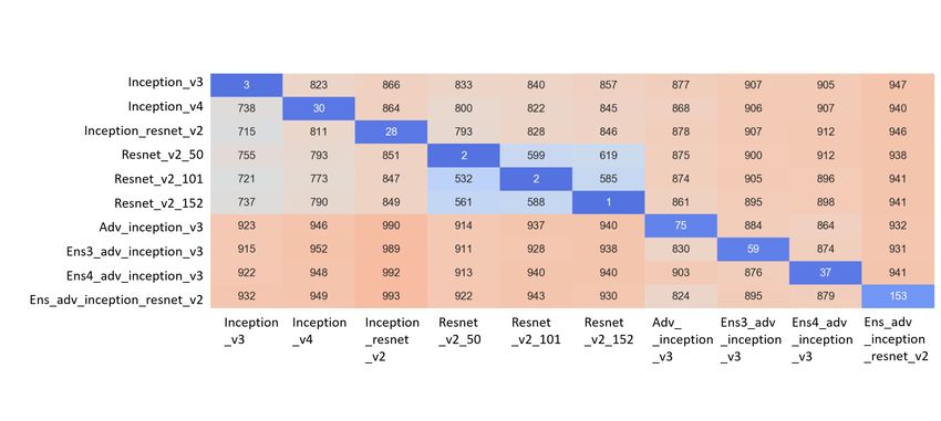
2                                                                         Kurakin et al.

structure and organization of the competition and the solutions developed by sev-
eral of the top-placing teams.

1 Introduction

Recent advances in machine learning and deep neural networks enabled researchers
to solve multiple important practical problems like image, video, text classification
and others.
    However most existing machine learning classifiers are highly vulnerable to ad-
versarial examples [2, 39, 15, 29]. An adversarial example is a sample of input data
which has been modified very slightly in a way that is intended to cause a machine
learning classifier to misclassify it. In many cases, these modifications can be so
subtle that a human observer does not even notice the modification at all, yet the
classifier still makes a mistake.
    Adversarial examples pose security concerns because they could be used to per-
form an attack on machine learning systems, even if the adversary has no access to
the underlying model.
    Moreover it was discovered [22, 33] that it is possible to perform adversarial
attacks even on a machine learning system which operates in physical world and
perceives input through inaccurate sensors, instead of reading precise digital data.
    In the long run, machine learning and AI systems will become more powerful.
Machine learning security vulnerabilities similar to adversarial examples could be
used to compromise and control highly powerful AIs. Thus, robustness to adversar-
ial examples is an important part of the AI safety problem.
    Research on adversarial attacks and defenses is difficult for many reasons. One
reason is that evaluation of proposed attacks or proposed defenses is not straightfor-
ward. Traditional machine learning, with an assumption of a training set and test set
that have been drawn i.i.d., is straightforward to evaluate by measuring the loss on
the test set. For adversarial machine learning, defenders must contend with an open-
ended problem, in which an attacker will send inputs from an unknown distribution.
It is not sufficient to benchmark a defense against a single attack or even a suite of
attacks prepared ahead of time by the researcher proposing the defense. Even if the
defense performs well in such an experiment, it may be defeated by a new attack that
works in a way the defender did not anticipate. Ideally, a defense would be provably
sound, but machine learning in general and deep neural networks in particular are
difficult to analyze theoretically. A competition therefore gives a useful intermediate
form of evaluation: a defense is pitted against attacks built by independent teams,
with both the defense team and the attack team incentivized to win. While such an
evaluation is not as conclusive as a theoretical proof, it is a much better simulation
of a real-life security scenario than an evaluation of a defense carried out by the
proposer of the defense.
    In this report, we describe the NIPS 2017 competition on adversarial attack and
defense, including an overview of the key research problems involving adversarial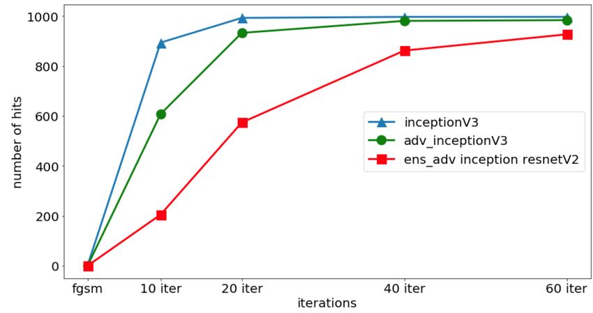
This is a preprint of a Springer book chapter from the “NIPS 2017 Competition Book”   3

examples (section 2), the structure and organization of the competition (section 3),
and several of the methods developed by the top-placing competitors (section 4).

2 Adversarial examples

Adversarial examples are inputs to machine learning models that have been inten-
tionally optimized to cause the model to make a mistake. We call an input example
a “clean example” if it is a naturally occurring example, such as a photograph from
the ImageNet dataset. If an adversary has modified an example with the intention
of causing it to be misclassified, we call it an “adversarial example.” Of course, the
adversary may not necessarily succeed; a model may still classify the adversarial ex-
ample correctly. We can measure the accuracy or the error rate of different models
on a particular set of adversarial examples.

2.1 Common attack scenarios

Scenarios of possible adversarial attacks can be categorized along different dimen-
sions.
   First of all, attacks can be classified by the type of outcome the adversary desires:
• Non-targeted attack. In this the case adversary’s goal is to cause the classifier
  to predict any inccorect label. The specific incorrect label does not matter.
• Targeted attack. In this case the adversary aims to change the classifier’s pre-
  diction to some specific target class.
   Second, attack scenarios can be classified by the amount of knowledge the ad-
versary has about the model:
• White box. In the white box scenario, the adversary has full knowledge of the
  model including model type, model architecture and values of all parameters and
  trainable weights.
• Black box with probing. In this scenario, the adversary does not know very
  much about the model, but can probe or query the model, i.e. feed some inputs
  and observe outputs. There are many variants of this scenario—the adversary
  may know the architecture but not the parameters or the adversary may not even
  know the architecture, the adversary may be able to observe output probabilities
  for each class or the adversary may only be to observe the choice of the most
  likely class.
• Black box without probing In the black box without probing scenario, the ad-
  versary has limited or no knowledge about the model under attack and is not
  allowed to probe or query the model while constructing adversarial examples.
  In this case, the attacker must construct adversarial examples that fool most ma-
  chine learning models.
4                                                                               Kurakin et al.

    Third, attacks can be classifier by the way adversary can feed data into the model:
• Digital attack. In this case, the adversary has direct access to the actual data
  fed into the model. In other words, the adversary can choose specific float32
  values as input for the model. In a real world setting, this might occur when an
  attacker uploads a PNG file to a web service, and intentionally designs the file to
  be read incorrectly. For example, spam content might be posted on social media,
  using adversarial perturbations of the image file to evade the spam detector.
• Physical attack. In the case of an attack in the physical world, the adversary
  does not have direct access to the digital representation of provided to the model.
  Instead, the model is fed input obtained by sensors such as a camera or micro-
  phone. The adversary is able to place objects in the physical environment seen
  by the camera or produce sounds heard by the microphone. The exact digital rep-
  resentation obtained by the sensors will change based on factors like the camera
  angle, the distance to the microphone, ambient light or sound in the environment,
  etc. This means the attacker has less precise control over the input provided to
  the machine learning model.

2.2 Attack methods

Most of the attacks discussed in the literature are geared toward the white-box digital
case.

2.2.1 White box digital attacks

L-BFGS . One of the first methods to find adversarial examples for neural networks
was proposed in [39]. The idea of this method is to solve the following optimization
problem:

           xadv − x → minimum,        s.t.   f (xadv ) = ytarget ,   xadv ∈ [0, 1]m       (1)
                   2
   The authors proposed to use the L-BFGS optimization method to solve this prob-
lem, thus the name of the attack.
   One of the main drawbacks of this method is that it is quite slow. The method
is not designed to counteract defenses such as reducing the number of bits used
to store each pixel. Instead, the method is designed to find the smallest possible
attack perturbation. This means the method can sometimes be defeated merely by
degrading the image quality, for example, by rounding to an 8-bit representation of
each pixel.
Fast gradient sign method (FGSM). To test the idea that adversarial examples
can be found using only a linear approximation of the target model, the authors of
[15] introduced the fast gradient sign method (FGSM).
This is a preprint of a Springer book chapter from the “NIPS 2017 Competition Book”    5

   FGSM works by linearizing loss function in L∞ neighbourhood of a clean im-
age and finds exact maximum of linearized function using following closed-form
equation:

                             xadv = x + ε sign ∇x J(x, ytrue )

                                                                                      (2)
Iterative attacks The L-BFGS attack has a high success rate and high compu-
tational cost. The FGSM attack has a low success rate (especially when the de-
fender anticipates it) and low computational cost. A nice tradeoff can be achieved
by running iterative optimization algorithms that are specialized to reach a solution
quickly, after a small number (e.g. 40) of iterations.
    One strategy for designing optimization algorithms quickly is to take the FGSM
(which can often reach an acceptable solution in one very large step) and run it for
several steps but with a smaller step size. Because each FGSM step is designed to
go all the way to the edge of a small norm ball surrounding the starting point for
the step, the method makes rapid progress even when gradients are small. This leads
to the Basic Iterative Method (BIM) method introduced in [23], also sometimes
called Iterative FGSM (I-FGSM):
                                      n                                     o
           x0adv = X , xN+1
                         adv
                             = ClipX,ε X adv
                                          N   +  α sign ∇X   X
                                                           J(X adv
                                                               N   , ytrue )      (3)

  The BIM can be easily made into a target attack, called the Iterative Target Class
Method:

                                      n                                o
        X adv
          0 = X,       X adv             adv
                                                         X adv
                         N+1 = ClipX,ε X N − α sign ∇X J(X N , ytarget )              (4)

   It was observed that with sufficient number of iterations this attack almost always
succeeds in hitting target class [23].
Madry et. al’s Attack [27] showed that the BIM can be significantly improved
by starting from a random point within the ε norm ball. This attack is often called
projected gradient descent, but this name is somewhat confusing because (1) the
term “projected gradient descent” already refers to an optimization method more
general than the specific use for adversarial attack, (2) the other attacks use the
gradient and perform project in the same way (the attack is the same as BIM except
for the starting point) so the name doesn’t differentiate this attack from the others.
Carlini and Wagner attack (C&W). N. Carlini and D. Wagner followed a path
of L-BFGS attack. They designed a loss function which has smaller values on ad-
versarial examples and higher on clean examples and searched for adversarial ex-
amples by minimizing it [6]. But unlike [39] they used Adam [21] to solve the
optimization problem and dealt with box constraints either by change of variables
(i.e. x = 0.5(tanh(w) + 1)) or by projecting results onto box constraints after each
step.
    They explored several possible loss functions and achieved the strongest L2 at-
tack with following: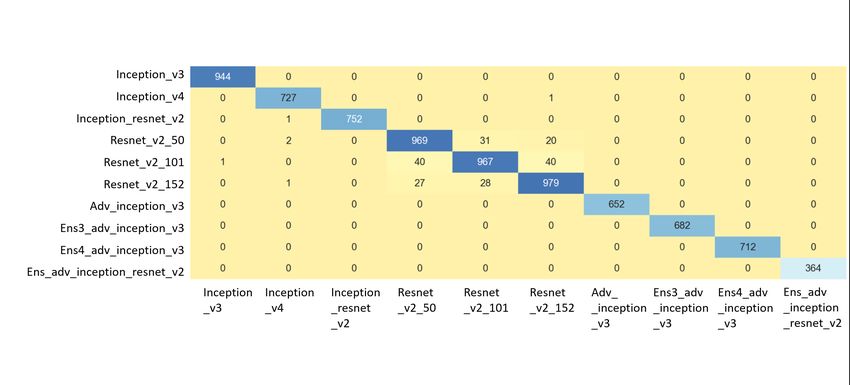
6                                                                         Kurakin et al.

          kxadv − xk p + c max max f (xadv )i − f (xadv )Y , −κ → minimum

                                                                                    (5)
                                i6=Y

where xadv parametrized 0.5(tanh(w) + 1); Y is a shorter notation for target class
ytarget ; c and κ are method parameters.
Adversarial transformation networks (ATN). Another approach which was ex-
plored in [1] is to train a generative model to craft adversarial examples. This model
takes a clean image as input and generates a corresponding adversarial image. One
advantage of this approach is that, if the generative model itself is designed to be
small, the ATN can generate adversarial examples faster than an explicit optimiza-
tion algorithm. In theory, this approach can be faster than even the FGSM, if the
ATN is designed to use less computation is needed for running back-propagation on
the target model. (The ATN does of course require extra time to train, but once this
cost has been paid an unlimited number of examples may be generated at low cost)
Attacks on non differentiable systems. All attacks mentioned about need to com-
pute gradients of the model under attack in order to craft adversarial examples.
However this may not be always possible, for example if model contains non-
differentiable operations. In such cases, the adversary can train a substitute model
and utilize transferability of adversarial examples to perform an attack on non-
differentiable system, similar to black box attacks, which are described below.

2.2.2 Black box attacks

It was observed that adversarial examples generalize between different models [38].
In other words, a significant fraction of adversarial examples which fool one model
are able to fool a different model. This property is called “transferability” and is
used to craft adversarial examples in the black box scenario. The actual number of
transferable adversarial examples could vary from a few percent to almost 100%
depending on the source model, target model, dataset and other factors. Attackers in
the black box scenario can train their own model on the same dataset as the target
model, or even train their model on another dataset drawn from the same distribu-
tion. Adversarial examples for the adversary’s model then have a good chance of
fooling an unknown target model.
    It is also possible to intentionally design models to systematically cause high
transfer rates, rather than relying on luck to achieve transfer.
    If the attacker is not in the complete black box scenario but is allowed to use
probes, the probes may be used to train the attacker’s own copy of the target
model [30, 29] called a “substitute.” This approach is powerful because the input
examples sent as probes do not need to be actual training examples; instead they can
be input points chosen by the attacker to find out exactly where the target model’s
decision boundary lies. The attacker’s model is thus trained not just to be a good
classifier but to actually reverse engineer the details of the target model, so the two
models are systematically driven to have a high amount of transfer.
This is a preprint of a Springer book chapter from the “NIPS 2017 Competition Book” 7
In the complete black box scenario where the attacker cannot send probes, one
strategy to increase the rate of transfer is to use an ensemble of several models as
the source model for the adversarial examples [26]. The basic idea is that if an ad-
versarial example fools every model in the ensemble, it is more likely to generalize
and fool additional models.
Finally, in the black box scenario with probes, it is possible to just run optimiza-
tion algorithms that do not use the gradient to directly attack the target model [3, 7].
The time required to generate a single adversarial example is generally much higher
than when using a substitute, but if only a small number of adversarial examples are
required, these methods may have an advantage because they do not have the high
initial fixed cost of training the substitute.
2.3 Overview of defenses
No method of defending against adversarial examples is yet completely satisfactory.
This remains a rapidly evolving research area. We given an overview of the (not yet
fully succesful defense methods) proposed so far.
Since adversarial perturbations generated by many methods look like high-
frequency noise to a human observer1 multiple authors have suggested to use im-
age preprocessing and denoising as a potential defence against adversarial exam-
ples. There is a large variation in the proposed preprocessing techniques, like doing
JPEG compression [9] or applying median filtering and reducing precision of input
data [43]. While such defences may work well against certain attacks, defenses in
this category have been shown to fail in the white box case, where the attacker is
aware of the defense [19]. In the black box case, this defense can be effective in
practice, as demonstrated by the winning team of the defense competition. Their
defense, described in section 5.1, is an example of this family of denoising strate-
gies.
Many defenses, intentionally or unintentionally, fall into a category called “gradi-
ent masking.” Most white box attacks operate by computing gradients of the model
and thus fail if it is impossible to compute useful gradients. Gradient masking con-
sists of making the gradient useless, either by changing the model in some way that
makes it non-differentiable or makes it have zero gradients in most places, or make
the gradients point away from the decision boundary. Essentially, gradient masking
means breaking the optimizer without actually moving the class decision boundaries
substantially. Because the class decision boundaries are more or less the same, de-
fenses based on gradient masking are highly vulnerable to black box transfer [30].
Some defense strategies (like replacing smooth sigmoid units with hard threshold
units) are intentionally designed to perform gradient masking. Other defenses, like
1 This may be because the human perceptual system finds the high-frequency components to be
more salient; when blurred with a low pass filter, adversarial perturbations are often found to have
significant low-frequency components8 Kurakin et al.
many forms of adversarial training, are not designed with gradient masking as a
goal, but seem to often learn to do gradient masking when applied in practice.
Many defenses are based on detecting adversarial examples and refusing to clas-
sify the input if there are signs of tampering [28]. This approach works long as the
attacker is unaware of the detector or the attack is not strong enough. Otherwise the
attacker can construct an attack which simultaneously fools the detector into think-
ing an adversarial input is a legitimate input and fools the classifier into making the
wrong classification [5].
Some defenses work but do so at the cost of seriously reducing accuracy on
clean examples. For example, shallow RBF networks are highly robust to adversarial
examples on small datasets like MNIST [16] but have much worse accuracy on clean
MNIST than deep neural networks. Deep RBF networks might be both robust to
adversarial examples and accurate on clean data, but to our knowledge no one has
successfully trained one.
Capsule networks have shown robustness to white box attacks on the Small-
NORB dataset, but have not yet been evaluated on other datasets more commonly
used in the adversarial example literature [13].
The most popular defense in current research papers is probably adversarial train-
ing [38, 15, 20]. The idea is to inject adversarial examples into training process and
train the model either on adversarial examples or on mix of clean and adversarial
examples. The approach was successfully applied to large datasets [24], and can be
made more effective by using discrete vector code representations rather than real
number representations of the input [4]. One key drawback of adversarial training
is that it tends to overfit to the specific attack used at training time. This has been
overcome, at least on small datasets, by adding noise prior to starting the optimizer
for the attack [27]. Another key drawback of adversarial training is that it tends to
inadvertently learn to do gradient masking rather than to actually move the decision
boundary. This can be largely overcome by training on adversarial examples drawn
from an ensemble of several models [40]. A remaining key drawback of adversarial
training is that it tends to overfit to specific constraint region used to generate the
adversarial examples (models trained to resist adversarial examples in a max-norm
ball may not resist adversarial examples based on large modifications to background
pixels [14] even if the new adversarial examples do not appear particularly challeng-
ing to a human observer).
3 Adversarial competition
The phenomenon of adversarial examples creates a new set of problems in machine
learning. Studying these problems is often difficult, because when a researcher pro-
poses a new attack, it is hard to tell whether their attack is strong, or whether they
have not implemented their defense method used for benchmarking well enough.
Similarly, it is hard to tell whether a new defense method works well or whether it
has just not been tested against the right attack.This is a preprint of a Springer book chapter from the “NIPS 2017 Competition Book” 9 To accelerate research in adversarial machine learning and pit many proposed at- tacks and defenses against each other in order to obtain the most vigorous evaluation possible of these methods, we decided to organize a competition. In this competition participants are invited to submit methods which craft ad- versarial examples (attacks) as well as classifiers which are robust to adversarial eaxmples (defenses). When evaluating competition, we run all attack methods on our dataset to produce adversarial examples and then run all defenses on all gener- ated adversarial examples. Attacks are ranked by number of times there were able to fool defenses and defenses are scored by number of correctly classified examples. 3.1 Dataset When making a dataset for these competition we had following requirements: 1. Large enough dataset and non-trivial problem, so the competition would be in- teresting. 2. Well known problem, so people potentially can reuse existing classifiers. (This ensures that competitors are able to focus on the adversarial nature of the chal- lenge, rather than spending all their time coming up with a solution to the under- lying task) 3. Data samples which were never used before, so participants unlikely to overfit to well known dataset. These requirements were satisfied by choosing image classification problem and creating a dataset with ImageNet-compatible images [10]. To do this we collected a set of images which were never used in publicly available datasets, labelled them using pretrained ImageNet classifier and then manually verified that these labels are correct. The original (non-adversarial) ImageNet challenge [32] is a complex and in- teresting problem, and thus satisfies requirement number 1. Additionally there are plenty of existing classifiers for ImageNet data, which satisfies requirement number 2. Because we collected new images and labelled them instead of using the already available dataset, our approach satisfies requirement number 3. Overall we collected two datasets for this competitions: • DEV dataset was released to participants in the beginning of the competition, so they can use it for development of their solutions. This dataset contained 1000 images. • FINAL dataset was kept secret and was used to evaluate final submissions of participants. It contained 5000 images.
10                                                                         Kurakin et al.

3.2 Tasks and competition rules

Our competition had three tracks. Each track had a different task:

• Non-targeted adversarial attack. In this track participants were invited to sub-
  mit a method which performs a non-targeted black box attack, i.e. given an in-
  put image, generate an adversarial image which is likely be misclassified by un-
  known classifier.
• Targeted adversarial attack. In this track participants were invited to submit a
  method which performs a targeted black box attack, i.e. given an input image and
  a target class, generate an adversarial image which is likely be misclassified as a
  given target class by unknown classifier.
• Defense against adversarial attacks. In this track, participants were invited to
  submit a classifier which is robust to adversarial examples.
   In all tracks participants submitted a program which performs the given task and
we ran this code using our evaluation infrastructure.
   The submitted program was given a set of images (and target classes in case of
targeted attack) as an input, and had to produce either an adversarial image (for
attack submission) or classification label (for defense submission) for each input
image.
   Input images were fed to each submission in batches of 100 images. To limit the
budget required for computation, the rules of the competitions specified that each
submission had to process a batch of 100 images in no more than 500 seconds. If a
submission was not done after 500 seconds, then processing of the current batch was
interrupted and the submission was fed the next batch. Only successfully processed
images were included in the score of the submission (see details below in evaluation
sub-section).

3.3 Evaluation metrics

An attack got 1 point each time it was able to fool a defense on single image. If
attack was unable to fool a defense or if it failed to generate an adversarial version
of an image within the time limit then it got 0 points for that image. A defense got
1 point for each correctly classified image and 0 points for incorrect classification
or failure to produce a classification label. A defense was used to score attacks only
if it successfully processed all input images, so that attackers were neither rewarded
nor penalized for making images that caused the defender to crash or time out—the
competition is purely about classification accuracy. Likewise, an attack was used to
score defenses only if it succesfully processed all inputs. Points for each submission
were added together and then normalized (using the same normalization constant
for all submissions), such that final scores of all submissions are in the range [0, 1],
where 1 means success on all images and 0 means failure on all images.
This is a preprint of a Springer book chapter from the “NIPS 2017 Competition Book”   11

   Specifically, the score of each non-targeted attack a(Image) was computed using
the following formula:
                                    N
                            1
                                ∑  ∑  [d(a(Ik )) 6= TrueLabelk ]                      (6)
                          |D|N d∈D k=1
   The score of each targeted attack a(Image, TargetLabel) was computed as:
                           N
                   1
                       ∑  ∑  [d(a(Ik , TargetLabelk )) = TargetLabelk ]               (7)
                 |D|N d∈D k=1
   The score of each defense d(Image) was computed in the following way:
                                    N
                            1
                               ∑ ∑ [d(a(Ik )) = TrueLabelk ]
                          |A|N a∈A
                                                                                      (8)
                                   k=1

   Where:
• A is the set of all attacks (targeted and non-targeted) which were used for evalua-
  tion of defenses (attacks that crashed on some inputs or ran out of time for some
  inputs were not used to evaluate defense);
• D is the set of all defenses which were used for evaluation of attacks (defenses
  that crashed on some inputs or ran out of time for some inputs were not used to
  evaluate attacks);
• N is the number of images in the dataset;
• Ik is the k-th image from the dataset;
• TrueLabelk is the true label of image Ik ;
• TargetLabelk is the chosen target label for image k;
• [P] is an indicator function which equals to 1 when P is true, and 0 when P is
  false or undefined.
• d(•) is a defending classifier. If the binary fails to complete execution within the
  time limit, the output of d(•) is a null label that never equals the true label. If
  d(•) is called on an undefined image, it is defined to always return the true label,
  so an attacker that crashes receives zero points.
   Additionally to metrics used for ranking, after the competition we computed
worst case score for each submission in defense and non-targeted attack tracks.
These scores were useful to understand how submissions act in the worst case. To
compute worst score of defense we computed accuracy of the defense against each
attack and chosen minimum:
                                  N
                           1
                             min ∑ [d(a(Ik )) = TrueLabelk ]                          (9)
                           N a∈A k=1
   To compute worst case score of non-targeted attack we computed how often at-
tack caused misclassification when used against each defense and chosen minimum
misclassification rate:
12 Kurakin et al.
N
1
min ∑ [d(a(Ik )) 6= TrueLabelk ] (10)
N d∈D k=1
Worst case score of targeted attack could be computed in a similar way, but gen-
erally not useful because targeted attacks are much weaker than non-targeted and all
worst scores of targeted attacks were 0.
3.4 Competition schedule
The competition was announced in May 2017, launched in the beginning of July
2017 and finished on October 1st, 2017. The ompetition was run in multiple rounds.
There were three development rounds followed by the final round:
• August 1, 2017 - first development round
• September 1, 2017 - second development round
• September 15, 2017 - third development round
• October 1, 2017 - deadline for final submission
Development rounds were optional and their main purpose was to help partici-
pants to test their solution. Only the final round was used to compute final scores of
submissions and determine winners.
All rounds were evaluated in a similar way. For the evaluation of the round we
gathered all submissions which were submitted before the round deadline, ran all of
them and computed scores as described in section 3.3.
We used DEV dataset to compute scores in development rounds and secret FI-
NAL dataset to compute scores in the final round.
3.5 Technical aspects of evaluation
Competition participants were submitting pieces of code and we have run them
ourselves. This approach posess several challanges. First of all we need to protect
competition infrastructure from malicious code. Secondly, given the dataset size and
number of submissions we had to run it in an efficient way.
We partnered with Kaggle2 and used their platform as a frontend for the com-
petition. Kaggle hosted competition web-site, leaderboard and participants were
uploading submissions through Kaggle. For evaluation of each round we took all
submissions from Kaggle and fed them into our evaluation infrastructure.
Evaluation infrastructure worked as described in algorithm 1. As could be seen
from the algorithm, attacks could be run independently of each other. Same for
defenses. We took advantage of this fact and parallelized execution of all attacks
and all defenses by spreading them across multiple machines.
2 www.kaggle.comThis is a preprint of a Springer book chapter from the “NIPS 2017 Competition Book” 13
Algorithm 1 Algorithm of work of evaluation infrastructure
. PREPARE DATASET
1: Split dataset D = {I1 , . . . , IN } into batches {B1 , . . . , Bk }, such that each batch Bi contains 100
image {I100(i−1)+1 , . . . , I100i }.
2: Assign size of maximum allowed perturbation εi to each batch Bi . Value of εi is randomly
4 8 12 16
chosen from the set { 255 , 255 , 255 , 255 }
. RUN ALL ATTACKS
3: for all b ∈ {1, . . . , k} do . loop over all batches, b is batch index
4: for all non-targeted attacks a do
5: Run attack a on batch Bb and generate a batch of adversarial images B̂ab . Size of maxi-
mum perturbation εb is provided to an attack.
6: Project each adversarial image from B̂ab into L∞ εb -neighborhood of corresponding
clean image from Bb .
7: end for
8: for all targeted attacks t do
9: Run attack t on batch Bb and generate a batch of adversarial images B̂tb . Attack is
provided with size of maximum perturbation εb as well as target classes for each
image from the batch Bb .
10: Project each adversarial image from B̂tb into L∞ εb -neighborhood of corresponding
clean image from Bb .
11: end for
12: end for
. RUN ALL DEFENSES
13: for all b ∈ {1, . . . , k} do . loop over all batches, b is batch index
14: for all defense d do
15: for all non-targeted attacks a do
16: Run defense d on all images from batch B̂ab
17: end for
18: for all targeted attacks t do
19: Run defense d on all images from batch B̂tb
20: end for
21: end for
22: end for
. COMPUTE SCORES
23: Determine subset of targeted and non-targeted attacks A which produces all adversarial images
24: Determine subset of defenses D which output classification labels for all input images
25: Compute scores of all submissions using equations 6, 7, 8
For final evaluation we used 100 Google Cloud VMs. At any given moment one
VM was running either one attack on one batch from the dataset or one defense on
one batch of adversarial images. Submissions were run inside Docker containers to
isolate submissions from our evaluation infrastructure and from the outside world.
4 Competition results
For the final round we had 91 non-targeted attack submissions, 65 targeted attack
submission and 107 defense submissions. During the course of competitions sub-14 Kurakin et al.
score improvement over baseline
0.45
score improvement over baseline
0.20
0.40
0.15 0.35
0.10 0.30
0.25
0.05
0.20
0.00 0.15
0.10
0.05
0.05
0.10 0.00
DEV1 DEV2 DEV3 FINAL DEV1 DEV2 DEV3 FINAL
round round
(a) Defenses (b) Non-targeted attacks
score improvement over baseline 0.25
0.20
0.15
0.10
0.05
0.00
DEV1 DEV2 DEV3 FINAL
round
(c) Targeted attacks
Fig. 1: Plots which shows difference between score of top submission and best base-
line in each round in each track. As could be seen from the plot, submissions kept
improving each round.
missions kept improving their results compared to baselines which could be seen
from Figure 1.
Final results of the top submissions in each track are provided in tables 1, 2 and 3.
Meaning of the columns is following. Rank is submission rank in final scoring,
score is submission score as described in Section 3.3, raw score is un-normalized
score which is number of times submission got a point on the image, worst score is
submission score in the worst case and medial eval time is median time needed for
evaluation of one batch of 100 images. To put things into prospective, plots of all
submission scores in final round from best to worst and comparison with provided
baselines are depicted in Figure 2.
As could be seen from the tables, best defenses achieved more than 90% accuracy
on all adversarial images from all attacks. At the same time worst case scores of
defenses are much lower. The highest worst case score among all defenses is only
53.6%.
This could be an indication that it’s possible to achieve pretty high accuracy
against adversarial examples in average case, however model will still be suspectible
to adversarial examples and could be fooled if adversary will be able to find them.This is a preprint of a Springer book chapter from the “NIPS 2017 Competition Book” 15
Table 1: Top-5 defense submissions, best baseline and submission with maximum
worst-case score
Rank Team name or baseline Score Raw Score Worst Score Median eval time
1 TSAIL 0.953164 691044 0.1184 51.0
2 iyswim 0.923524 669555 0.2520 126.0
3 Anil Thomas 0.914840 663259 0.2666 97.0
4 erko 0.911961 661172 0.2920 87.0
5 Stanford & Suns 0.910593 660180 0.0682 129.0
24 Rafael Moraes 0.871739 632011 0.5358 17.0
56 Baseline (Ens. adv. ir v2) 0.772908 560358 0.0186 17.0
Table 2: Top-5 non-targeted attack submissions, best baseline and best submission
with according to worst-case score.
Rank Team name or baseline Score Raw Score Worst Score Median eval time
1 TSAIL 0.781644 410363 0.1364 423.0
2 Sangxia 0.776855 407849 0.3412 421.0
3 Stanford & Sun 0.774025 406363 0.2722 497.0
4 iwiwi 0.768981 403715 0.1352 76.0
5 toshi k 0.755598 396689 0.3322 448.0
44 Baseline (FGSM) 0.346400 181860 0.0174 17.0
Table 3: Top-5 targeted attack submissions and best baseline.
Rank Team Score Raw Score Median Eval Time
1 TSAIL 0.402211 211161.0 392.0
2 Sangxia 0.368773 193606.0 414.0
3 FatFingers 0.368029 193215.0 493.0
4 Anil Thomas 0.364552 191390.0 495.0
5 WNP 0.347935 182666.0 487.0
24 Baseline (Iter. T. C. 20) 0.199773 104881.0 127.0
Similar observation holds for attacks. Best attacks achieved up to 78% fooling
rate against all defenses, at the same time worst case score of attacks was no more
than 34%.
5 Top scoring submissions
In the remainder of the chapter, we present the solutions of several of the top-scoring
teams.
To describe the solutions, we use the following notation:16 Kurakin et al.
1.0 1.0
FGSM
0.8 0.8 Random noise
No op
0.6 0.6 all scores
score
score
0.4 0.4
ensemble ir_v2
adv inc_v3
0.2 inc_v3 0.2
all scores
0.0 0.0
0 20 40 60 80 100 0 20 40 60 80
rank rank
(a) Defenses (b) Non-targeted attacks
1.0
Iter. T.C., 20
0.8 Iter. T.C., 10
Step T.C.
0.6 all scores
score
0.4
0.2
0.0
0 10 20 30 40 50 60
rank
(c) Targeted attacks
Fig. 2: Plots with scores of submissions in all three tracks. Solid line of each plot
is scores of submissions depending on submission rank. Dashed lines are scores of
baselines we provided. These plots demonstrate difference between best and worst
submissions as well as how much top submissions were able to improve provided
baselines.
• x - input image with label ytrue . Different images are distinguished by super-
scripts, for examples images x1 , x2 , . . . with labels ytrue
1 , y2 , . . ..
true
• ytarget is a target class for image x for targeted adversarial attack.
• Functions with names like f (•), g(•), h(•), . . . are classifiers which map input
images into logits. In other words f (x) is logits vector of networks f on image x
• J( f (x), y) - cross entropy loss between logits f (x) and class y.
• ε - maximum L∞ norm of adversarial perturbation.
• xadv - adversarial images. For iterative methods xadv i is adversarial example gen-
erated on step i.
• Clip[a,b] (•) is a function which performs element-wise clipping of input tensor
to interval [a, b].
• X is the set of all training examples.
All values of images are normalized to be in [0, 1] interval. Values of ε are also
16
normalized to [0, 1] range, for examples ε = 255 correspond to uint8 value of epsilon
equal to 16.This is a preprint of a Springer book chapter from the “NIPS 2017 Competition Book” 17
5.1 1st place in defense track: team TsAIL
Team members: Yinpeng Dong, Fangzhou Liao, Ming Liang, Tianyu Pang, Jun
Zhu and Xiaolin Hu.
In this section, we introduce the high-level representation guided denoiser (HGD)
method, which won the first place in the defense track. The idea is to train a neural
network based denoiser to remove the adversarial perturbation.
5.1.1 Dataset
To prepare the training set for the denoiser, we first extracted 20K images from the
ImageNet training set (20 images per class). Then we used a bunch of adversarial
attacks to distort these images and form a training set. Attacking methods included
FGSM and I-FGSM and were applied to the many models and their ensembles to
simulate weak and strong attacks.
5.1.2 Denoising U-net
Denoising autoencoder (DAE) [41] is a potential choice of the denoising network.
But DAE has a bottleneck for the transmission of fine-scale information between the
encoder and decoder. This bottleneck structure may not be capable of carrying the
multi-scale information contained in the images. That’s why we used a denoising
U-net (DUNET).
Compared with DAE, the DUNET adds some lateral connections from encoder
layers to their corresponding decoder layers of the same resolution. In this way,
the network is learning to predict adversarial noise only, which is more relevant to
denoising and easier than reconstructing the whole image [44]. The clean image can
be readily obtained by subtracting the noise from the corrupted input:
d x̂ = Dw (xadv ). (11)
x̂ = xadv − d x̂. (12)
where Dw is a denoiser network with parameters w, d x̂ is predicted adversarial noise
and x̂ is reconstructured clean image.
5.1.3 Loss function
The vanilla denoiser uses the reconstructing distance as the loss function, but we
found a better method. Given a target neural network, we extract its representation
at l-th layer for x and x̂, and calculate the loss function as:
L = k fl (x̂) − fl (x)k1 . (13)18 Kurakin et al.
The corresponding models are called HGD, because the supervised signal comes
from certain high-level layers of the classifier and carries guidance information re-
lated to image classification.
We propose two HGDs with different choices of l. For the first HGD, we define
l = −2 as the index of the topmost convolutional layer. This denoiser is called fea-
ture guided denoiser (FGD). For the second HGD, we use the logits layer. So it is
called logits guided denoiser (LGD).
Another kind of HGD uses the classification loss of the target model as the de-
noising loss function, which is supervised learning as ground truth labels are needed.
This model is called class label guided denoiser (CGD). In this case the loss function
is optimized with respect to the parameters of the denoiser w, while the parameters
of the guiding model are fixed.
Please refer to our full-length paper [25] for more information.
5.2 1st place in both attack tracks: team TsAIL
Team members: Yinpeng Dong, Fangzhou Liao, Ming Liang, Tianyu Pang, Jun
Zhu and Xiaolin Hu.
In this section, we introduce the momentum iterative gradient-based attack
method, which won the first places in both the non-targeted attack and targeted
attack tracks. We first describe the algorithm in Sec. 5.2.1, and then illustrate our
submissions for non-targeted and targeted attacks respectively in Sec. 5.2.2 and
Sec. 5.2.3. A more detailed description can be found in [11].
5.2.1 Method
The momentum iterative attack method is built upon the basic iterative method [23],
by adding a momentum term to greatly improve the transferability of the generated
adversarial examples.
Existing attack methods exhibit low efficacy when attacking black-box models,
due to the well-known trade-off between the attack strength and the transferabil-
ity [24]. In particular, one-step method (e.g., FGSM) calculates the gradient only
once using the assumption of linearity of the decision boundary around the data
point. However in practice, the linear assumption may not hold when the distortions
are large [26], which makes the adversarial examples generated by one-step method
“underfit” the model, limiting attack strength. In contrast, basic iterative method
greedily moves the adversarial example in the direction of the gradient in each iter-
ation. Therefore, the adversarial example can easily drop into poor local optima and
“overfit” the model, which are not likely to transfer across models.
In order to break such a dilemma, we integrate momentum [31] into the basic
iterative method for the purpose of stabilizing update directions and escaping from
poor local optima, which are the common benefits of momentum in optimizationThis is a preprint of a Springer book chapter from the “NIPS 2017 Competition Book” 19
literature [12, 34]. As a consequence, it alleviates the trade-off between the attack
strength and the transferability, demonstrating strong black-box attacks.
The momentum iterative method for non-targeted attack is summarized as:
∇x J( f (xtadv ), ytrue )
gt+1 = µ · gt + , xt+1 = Clip[0,1] (xtadv + α · sign(gt+1 )) (14)
k∇x J( f (xtadv ), ytrue )k1 adv
where g0 = 0, xadv
0 = x, α = ε with T being the number of iterations. gt gathers the
T
gradients of the first t iterations with a decay factor µ and adversarial example xtadv
is perturbed in the direction of the sign of gt with the step size α. In each iteration,
the current gradient ∇x J( f (xtadv ), ytrue ) is normalized to have unit L1 norm (however
other norms will work too), because we noticed that the scale of the gradients varies
in magnitude between iterations.
To obtain more transferable adversarial examples, we apply the momentum iter-
ative method to attack an ensemble of models. If an example remains adversarial for
multiple models, it may capture an intrinsic direction that always fools these models
and is more likely to transfer to other models at the same time [26], thus enabling
powerful black-box attacks.
We propose to attack multiple models whose logit activations are fused together,
because the logits capture the logarithm relationships between the probability pre-
dictions, an ensemble of models fused by logits aggregates the fine detailed outputs
of all models, whose vulnerability can be easily discovered. Specifically, to attack
an ensemble of K models, we fuse the logits as
K
f (x) = ∑ wk fk (x) (15)
k=1
where fk (x) are the k-th model, wk is the ensemble weight with wk ≥ 0 and
∑Kk=1 wk = 1. Therefore we get a big ensemble model f (x) and we can use the mo-
mentum iterative method to attack f .
5.2.2 Submission for non-targeted attack
In non-targeted attack, we implemented the momentum iterative method for attack-
ing an ensemble of following models:
• Normally trained (i.e. without adversarial training) Inception v3 [37], Incep-
tion v4 [35], Inception Resnet v2 [35] and Resnet v2-101 [18] models.
• Adversarially trained Inception v3adv [24] model.
• Ensemble adversarially trained Inc-v3ens3 , Inc-v3ens4 and IncRes-v2ens models
from [40].
0.25 1
Ensemble weights (from Equation 15) were 7.25 for Inception-v3adv and 7.25 for
all other models. The number of iterations was 10 and the decay factor µ was 1.0.20 Kurakin et al.
5.2.3 Submission for targeted attack
For targeted attacks, we used a different formula of momentum iterative method:
∇x J( f (xtadv ), ytarget )
gt+1 = µ · gt + (16)
std(∇x J( f (xtadv ), ytarget )
xt+1 t
adv = Clip[0,1] xadv − α · Clip[−2,2] (round(g
t+1
)) (17)
where std(•) is the standard deviation and round(•) is rounding to nearest inte-
ger. Values of Clip[−2,2] (round(•)) are in set {−2, −1, 0, 1, 2} which enables larger
search space compared to sign function.
No transferability of the generated adversarial examples was observed in the tar-
geted attacks, so we implement our method for attacking several commonly used
white-box models.
We built two versions of the attacks. If the size of perturbation ε was smaller than
8 1 2
255 , we attacked ensemble of Inception v3 and IncRes-v2ens with weights 3 and 3 ;
otherwise we attacked an ensemble of Inception v3, Inception-v3adv , Inc-v3ens3 , Inc-
4 1 1 1 4
v3ens4 and IncRes-v2ens with ensemble weights 11 , 11 , 11 , 11 and 11 . The number of
iterations were 40 and 20 respectively, and the decay factor µ was 1.0.
5.3 2nd place in defense track: team iyswim
Team members: Cihang Xie, Jianyu Wang, Zhishuai Zhang, Zhou Ren and Alan
Yuille
In this submission, we propose to utilize randomization as a defense against
adversarial examples. Specifically, we propose a randomization-based method, as
shown in figure 3, which adds a random resizing layer and a random padding layer
to the beginning of the classification networks. Our method enjoys the following
advantages: (1) no additional training or fine-tuning; (2) very few additional com-
putations; (3) compatible with other adversarial defense methods. By combining the
proposed randomization method with an adversarially trained model, it ranked No.2
in the NIPS adversarial defense challenge.
Input Image x Resized Image x’ Padded Image x’’
Random Random
Resizing Padding
Layer Layer
Deep car
Network
Fig. 3: The pipeline of the proposed defense method. The input image x first goes
through the random resizing layer with a random scale applied. Then the random
padding layer pads the resized image x0 in a random manner. The resulting padded
image x00 is used for classification.This is a preprint of a Springer book chapter from the “NIPS 2017 Competition Book” 21 5.3.1 Randomization as defense Intuitively, the adversarial perturbation generated by iterative attacks may easily get over-fitted to the specific network parameters, and thus be less transferable. Due to this weak generalization ability, we hypothesis that low-level image transforma- tions, e.g., resizing, padding, compression, etc, may probably destroy the specific structure of adversarial perturbations, thus making it a good defense. It can even de- fend against white-box iterative attacks if random transformations are applied. This is because each test image goes through a transformation randomly and the attacker does not know this specific transformation when generating adversarial noise. 5.3.2 Randomization layers The first randomization layer is a random resizing layer, which resizes the origi- nal input image x with the size W × H × 3 to a new image x0 with random size W 0 × H 0 × 3. Note that, |W 0 −W | and |H 0 − H| should be within a reasonably small range, otherwise the network performance on clean images would significantly drop. Taking Inception-ResNet network [35] as an example, the original data input size is 299 × 299 × 3. Empirically we found that the network accuracy hardly drops if we control the height and width of the resized image x0 to be within the range [299, 331). The second randomization layer is the random padding layer, which pads zeros around the resized image in a random manner. Specifically, by padding the resized image x0 into a new image x00 with the size W 00 × H 00 × 3, we can choose to pad w zero pixels on the left, W 00 − W 0 − w zero pixels on the right, h zero pixels on the top and H 00 − H 0 − h zero pixels on the bottom. This results in a total number of (W 00 −W 0 + 1) × (H 00 − H 0 + 1) different possible padding patterns. During implementation, the original image first goes through two randomization layers, and then we pass the transformed image to the original CNN for classifica- tion. The pipeline is illustrated in figure 3. 5.3.3 Randomization layers + adversarial training Recently, adversarial training [24, 40] was developed as an effective defense for single-step attacks. Thus by adding the proposed random transformations as addi- tional layers to an adversarially trained model [40], it is expected that this method is able to effectively defend against both single-step and iterative attacks, including both black-box and white-box settings. 5.3.4 Submission details and results An adversarially trained model appended with randomization layers was submitted as our defense model to the challenge. Specifically, we (1) set the resizing range to
22                                                                              Kurakin et al.

be [310, 331); (2) set the padding size to be 331 × 331 × 3; (3) choose the adversar-
ially trained model to be ens-adv-Inception-Resnet-v23 ; (4) average the prediction
results over 30 randomization patterns for each image; (5) flip the input image with
probability 0.5 for each randomization pattern. The whole implementation is public
available4 .
    By evaluating our model against 156 different attacks, it reaches a normalized
score of 0.924 (ranked No.2 among 107 defense models), which is far better than
using ensemble adversarial training [40] alone with a normalized score of 0.773.
This result further demonstrates that the proposed randomization method can effec-
tively make deep networks much more robust to adversarial attacks.

5.3.5 Attackers with more information

When submitting the proposed defense method to the NIPS competition, the ran-
domization layers are remained as an unknown network module for the attackers.
We thus test the robustness of this defense method further by assuming that the at-
tackers are aware of the existence of randomization layers. Extensive experiments
are performed in [42], and it shows that the attackers still cannot break this defense
completely in practice. Interested readers can refer to [42] for more details.

5.4 2nd place in both attack tracks: team Sangxia

Team members: Sangxia Huang
   In this section, we present the submission by Sangxia Huang for both non-
targeted and targeted attacks. The approach is an iterated FGSM attack against an
ensemble of classifiers with random perturbations and augmentations for increased
robustness and transferability of the generated attacks. The source code is available
online. 5 We also optimize the iteration steps for improved efficiency as we describe
in more details below.
Basic idea An intriguing property of adversarial examples observed in many works
[30, 38, 16, 29] is that adversarial examples generated for one classifier transfer to
other classifiers. Therefore, a natural approach for effective attacks against unknown
classifiers is to generate strong adversarial examples against a large collection of
classifiers.
   Let f 1 , . . . , f k be an ensemble of image classifiers that we choose to target. In our
solution we give equal weights to each of them. For notation simplicity, we assume
that the inputs to all f i have the same size. Otherwise, we first insert a bi-linear

3 https://download.tensorflow.org/models/ens_adv_inception_resnet_
v2_2017_08_18.tar.gz
4 https://github.com/cihangxie/NIPS2017_adv_challenge_defense
5 https://github.com/sangxia/nips-2017-adversarial
This is a preprint of a Springer book chapter from the “NIPS 2017 Competition Book” 23
scaling layer, which is differentiable. The differentiability ensures that the correct
gradient signal is propagated through the scaling layer to the individual pixels of the
images.
Another idea we use to increase robustness and transferrability of the attacks
is image augmentation. Denote by Tθ an image augmentation function with pa-
rameter θ . For instance, we can have θ ∈ [0, 2π) as an angle and Tθ as the func-
tion that rotates the input image clock-wise by θ . The parameter θ can also be a
vector. For instance, we can have θ ∈ (0, ∞)2 as scaling factors in the width and
height dimension, and Tθ as the function that scales the input image in the width
direction by θ1 and in the height direction by θ2 . In our final algorithm, Tθ takes
the general form of a projective transformation with θ ∈ R8 as implemented in
tf.contrib.image.transform.
Let x be an input image, and ytrue be the label of x. Our attack algorithm works
to find an xadv that maximizes the expected average cross entropy loss of the predic-
tions of f 1 , . . . , f k over a random input augmentation 6
" #
1 k i
max
xadv :kx−xadv k∞ ≤ε
Eθ ∑ J f (Tθ (x)), ytrue .
k i=1
However, in a typical attack scenario, the true label ytrue is not available to the
attacker, therefore we substitute it with a psuedo-label ŷ generated by an image
classifer g that is available to the attacker. The objective of our attack is thus the
following
1 k
Eθ i J f i (Tθ i (x)), g(x) .
max ∑
x :kx−x k∞ ≤ε k i=1
adv adv
Using linearity of gradients, we write the gradient of the objective as
1 k
∑ ∇x Eθ i J f i (Tθ i (x)), g(x) .
k i=1
For typical distributions of θ , such as uniform or normal distribution, the gradient of
the expected cross entropy loss over a random θ is hard to compute. In our solution,
we replace it with an empirical estimate which is an average of the gradients for a
few samples of θ . We also adopt the approach in [40] where x is first randomly
perturbed. The use of random projective transformation seems to be a natural idea,
but to the best of our knowledge, this has not been explicitly described in previous
works on generating adversarial examples for image classifiers.
In the rest of this section, we use ∇bi (x) to denote the empirical gradient estimate
on input image x as described above.
0 := x, xmin = max(x − ε, 0), xmax = min(x + ε, 1), and let α 1 , α 2 , . . . be a
Let xadv
sequence of pre-defined step sizes. Then in the i-th step of the iteration, we update
the image by
6 The distribution we use for θ corresponds to a small random augmentation. See code for details.24 Kurakin et al.
! !
i i−1 1 k bi
xadv = clip xadv + α i sign min max
∑ ∇ (x) , x , x .
k i=1
Optimization We noticed from our experiments that non-targeted attacks against
pre-trained networks without defense (white-box and black-box) typically succeed
in 3 – 4 rounds, whereas attacks against adversarially trained networks take more
iterations. We also observed that in later iterations, there is little benefit in including
in the ensemble un-defended networks that have been successfully attacked. In the
final solution, each iteration is defined by step size α i as well as the set of classifiers
to include in the ensemble for the respective iteration. These parameters were found
through trial and error on the official development dataset of the competition.
Experiments: non-targeted attack We randomly selected 18,000 images from
ImageNet [32] for which Inception V3 [36] classified correctly.
The classifiers in the ensemble are: Inception V3 [36], ResNet 50 [17], ResNet
101 [17], Inception ResNet V2 [35], Xception [8], ensemble adversarially trained
Inception ResNet V2 (EnsAdv Inception ResNet V2) [40], and adversarially trained
Inception V3 (Adv Inception V3) [24].
We held out a few models to evaluate the transferrability of our attacks. The
holdout models listed in Table 4 are: Inception V4 [35], ensemble adversarially
trained Inception V3 with 2 (and 3) external models (Ens-3-Adv Inception V3, and
Ens-4-Adv Inception V3, respectively) [40].
Table 4: Success rate — non-targeted attack
Classifier Success rate
Inception V3 96.74%
ResNet 50 92.78%
Inception ResNet V2 92.32%
EnsAdv Inception ResNet V2 87.36%
Adv Inception V3 83.73%
Inception V4 91.69%
Ens-3-Adv Inception V3 62.76%
Ens-4-Adv Inception V3 58.11%
Table 4 lists the success rate for non-targeted attacks with ε = 16/255. The per-
formance for ε = 12/255 is similar, and somewhat worse for smaller ε. We see that
a decent amount of the generated attacks transfer to the two holdout adversarially
trained network Ens-3-Adv Inception V3 and Ens-4-Adv Inception V3. The transfer
rate for many other publicly available pretrained networks without defense are all
close to or above 90%. For brevity, we only list the performance on Inception V4
for comparison.
Targeted attack Our targeted attack follows a similar approach as non-targeted
attack. The main differences are:You can also read