Optimal control of the COVID 19 pandemic: controlled sanitary deconfinement in Portugal - Nature
←
→
Page content transcription
If your browser does not render page correctly, please read the page content below
www.nature.com/scientificreports
OPEN Optimal control of the COVID‑19
pandemic: controlled sanitary
deconfinement in Portugal
Cristiana J. Silva 1*, Carla Cruz 1, Delfim F. M. Torres 1, Alberto P. Muñuzuri
2
, Alejandro Carballosa 2, Iván Area 3, Juan J. Nieto 4, Rui Fonseca‑Pinto 5,
Rui Passadouro 5,6, Estevão Soares dos Santos 6, Wilson Abreu 7 & Jorge Mira 8*
The COVID-19 pandemic has forced policy makers to decree urgent confinements to stop a rapid
and massive contagion. However, after that stage, societies are being forced to find an equilibrium
between the need to reduce contagion rates and the need to reopen their economies. The experience
hitherto lived has provided data on the evolution of the pandemic, in particular the population
dynamics as a result of the public health measures enacted. This allows the formulation of forecasting
mathematical models to anticipate the consequences of political decisions. Here we propose a model
to do so and apply it to the case of Portugal. With a mathematical deterministic model, described
by a system of ordinary differential equations, we fit the real evolution of COVID-19 in this country.
After identification of the population readiness to follow social restrictions, by analyzing the social
media, we incorporate this effect in a version of the model that allow us to check different scenarios.
This is realized by considering a Monte Carlo discrete version of the previous model coupled via a
complex network. Then, we apply optimal control theory to maximize the number of people returning
to “normal life” and minimizing the number of active infected individuals with minimal economical
costs while warranting a low level of hospitalizations. This work allows testing various scenarios of
pandemic management (closure of sectors of the economy, partial/total compliance with protection
measures by citizens, number of beds in intensive care units, etc.), ensuring the responsiveness of the
health system, thus being a public health decision support tool.
COVID19 is an ongoing global concern. On March 11, 2020, the World Health Organization (WHO) declared
the state of pandemic due to SARS-COV2 infection and, worldwide, the containment strategies to control the
spread of COVID-19 were gradually intensified. In the first three months after COVID-19 emerged, nearly 1
million people were infected and 50,000 died. Although we had in the past similar diseases caused by the same
family of virus (e.g., SARS and MERS), these strategies are still of huge importance as the rate of spread of the
SARS-COV2 virus is higher1. The social and clinical experience with COVID-19 will leave lasting marks in soci-
ety and in the health system, from Latin cultural habits (proximity, touch, kiss) until health system configuration
changes, leaving hospitals for more complex clinical situations and providing community institutions (Health
Centers, Family Health Units and Integrated Continuous Care Units) with diagnostic and therapeutic means
that avoid systematic recourse to hospital emergencies.
By August 15, 2020, the cumulated number of confirmed cases by COVID-19 was of 21,387,974, with
14,169,695 recovered cases and 764,112 deaths, corresponding to 6,454,140 active cases (at a given time t, the
term “active infected” corresponds to the number of confirmed infected individuals active at that time t, while
the term “confirmed infected” corresponds to the accumulated number of confirmed infected individuals from
1
Department of Mathematics, Center for Research and Development in Mathematics and Applications (CIDMA),
University of Aveiro, 3810‑193 Aveiro, Portugal. 2Department of Physics, Institute CRETUS, Group of Nonlinear
Physics, Universidade de Santiago de Compostela, 15782 Santiago de Compostela, Spain. 3Departamento
de Matemática Aplicada II, E. E. Aeronáutica e do Espazo, Campus de Ourense, Universidade de Vigo,
32004 Ourense, Spain. 4Instituto de Matemáticas, Universidade de Santiago de Compostela, 15782 Santiago de
Compostela, Spain. 5Center for Innovative Care and Health Technology (ciTechCare), Polytechnic of Leiria, Leiria,
Portugal. 6ACES Pinhal Litoral-ARS Centro, Leiria, Portugal. 7School of Nursing and Research Centre “Centre for
Health Technology and Services Research/ESEP-CINTESIS”, Porto, Portugal. 8Departamento de Física Aplicada,
Universidade de Santiago de Compostela, 15782 Santiago de Compostela, Spain. *email: cjoaosilva@ua.pt;
jorge.mira@usc.es
Scientific Reports | (2021) 11:3451 | https://doi.org/10.1038/s41598-021-83075-6 1
Vol.:(0123456789)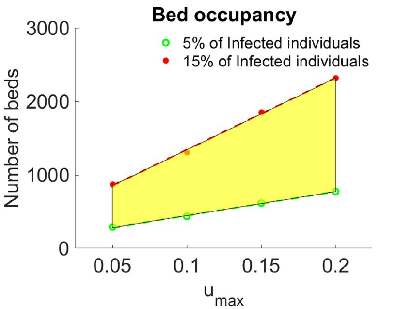
www.nature.com/scientificreports/
the beginning of the epidemic till time t). Regarding the active cases, 6,035,791 (99%) suffer mild condition of
the disease and 65,488 (1%) are in serious or critical health situation2. In Portugal, the first confirmed 2 infected
cases were reported on March 2, 2020, and the Government ordered public services to draw up a contingency
plan in line with the guidelines set by the Portuguese Public Health Authorities. On March 12, 2020, it was
declared State of Emergency. In the following week, additional measures were adopted, such as: prohibition of
events, meetings or gathering of people, regardless of reason or nature, with 100 or more people; prohibition of
drinking alcoholic beverages in public open-air spaces, except for outdoor areas catering and beverage estab-
lishments, duly licensed for the purpose; documentary control of people in borders; the suspension of all and
any activity of stomatology and dentistry, with the exception of proven urgent situations and non-postponable.
Teaching as well as non-teaching and classroom training activities were suspended from 16th March 20203; the air
traffic to and from Portugal was banned for all flights to and from countries that do not belong to the European
Union, with certain exceptions. Actually, the Portuguese were advised to stay at home, avoiding social contacts,
since 14th March 2020, inclusive, restricting to the maximum their exits from home. From March 20 on, it was
mandatory to adopt the teleworking regime, regardless of the employment relationship, whenever the functions
in question allow. On May 2 the emergency status was canceled (duration of 45 days). After the 45 days of state
of emergency, the Government progressively established measures for the reopening of the economy but with
rules for the control of the spread of the virus. Portugal is still in situation of alert, and the situation of calamity
and contingency can be declared, depending on the region and the number of active cases. According to the
Portuguese Health Authorities, as of the writing, there has not been an overload of intensive care services; since
the beginning of the Portuguese outbreak the intensive medicine capacity increased from 629 to 819 beds (+23%)
(data from June 14, 2020); the health authorities objective is to reach, by the end of 2020, a ratio of 9.4 beds per
100 thousand inhabitants. Moreover, Portugal did not enter a rupture situation; at the peak of the epidemic (in the
end of April, beginning of May), there were 1026 intensive care beds; the levels of intensive medicine occupancy,
by June 14, 2020, were of 61% at national level and 65% in the Lisbon and Vale do Tejo r egion4.
The way we manage today the pandemic is related to the ability to produce quality data, which in turn will
allow us to use the same data for mathematical modeling tasks, that are the best framework to deal with upcoming
scenarios5. Many efforts have been done in this fi eld6–9. The adjustment of the model parameters in a dynamic
way, through the imposition of limits on the system in order to optimize a given function, can be implemented
through the theory of optimal c ontrol10.
The usefulness of optimal control in epidemiology is well-known: while mathematical modeling of infectious
diseases has shown that combinations of isolation, quarantine, vaccination and/or treatment are often necessary
in order to eliminate an infectious disease, optimal control theory tell us how they should be administered, by
providing the right times for intervention and the right a mounts11,12. This optimization strategy has also been
used in some works within the scope of COVID-19. Optimal control of an adapted Susceptible–Exposure–Infec-
tion–Recovery (SEIR) model has been done with the aim to investigate the efficacy of two potential lockdown
release strategies on the UK p opulation13. Other COVID-19 case studies include the use of optimal control in
USA . Optimal administration of an hypothetical vaccine for COVID-19 has been also investigated15; and an
14
expression for the basic reproduction number in terms of the control variables o btained16. According to the
most recent pandemic spreading data, until a large immunization rate is achieved (ideally by a vaccine), the
application of so-called nonpharmaceutical interventions (NPIs) is the key to control the number of active
infected individuals17.
Here we are interested in using optimal control theory has a tool to understand ways to curtail the spread of
COVID-19 in Portugal by devising optimal disease intervention strategies. Moreover, we take into account several
important issues that have not yet been fully considered in the literature. Our model allows the application of
the theory of optimal control, to test containment scenarios in which the response capacity of health services is
maintained. Because the pandemic has shown that the public health concern is not only a medical problem, but
hole18, the dynamics of monitoring the containment measures, that allow each indi-
also affects society as a w
vidual to remain in the protected P class, is here obtained through models of analysis of social networks, which
differentiates this study getting closer to the real behavior of individuals and also predicting the adherence of
the population to possible government policies.
Results
Confirmed active infected individuals in Portugal. We propose a deterministic SAIRP mathematical
model for the transmission dynamics of SARS-CoV-2 in a homogeneous population, which is subdivided into
five compartments depending on the state of infection and disease of the individuals (see Supplementary Fig. 1):
S, susceptible (uninfected and not immune); A, infected but asymptomatic (undetected); I, active infected
(symptomatic and detected/confirmed); R, removed (recovered and deaths by COVID-19); P, protected/pre-
vented (not infected, not immune, but that are under protective measures).
The class P represents all individuals that practice, with daily efficacy, the so-called non-pharmaceutical
interventions (NPIs), e.g., physical distancing, use of face masks, and eye protection to prevent person-to-person
transmission of SARS-CoV-2 and COVID-19. Based on recent l iterature19,20, we assume that the individuals in
the class P are free from infection, but are not immune and, if they stop taking these measures, they become
susceptible again, at a rate ω = wm, where w represents the transition rate from protected P to susceptible S and
m represents the fraction of protected individuals that is transferred from P to S class (see Supplementary Fig. 1
for the diagram of the model; for the equations and a description of the parameters, see the “Methods” section).
In Fig. 1, we show that the SAIRP model (as described above and in detail in “Methods”) fits well the con-
firmed active infected cases in Portugal from March 2, 2020 until July 29, 2020 (a total of 150 days), using the
data from The Portuguese Public Health A uthorities21. More precisely, based on daily reports from the Portuguese
Scientific Reports | (2021) 11:3451 | https://doi.org/10.1038/s41598-021-83075-6 2
Vol:.(1234567890)www.nature.com/scientificreports/
10 -3 May17 May 24 June 9
2.5
Model: March 2 - May 17
Fraction of active infected
Model: May 17 - June 9
2 Model: June 9 - July 29
Real data
1.5
1
0.5
0
0 50 100 150
Time (days)
Figure 1. Fraction of confirmed active cases per day in Portugal. Red line: from March 2 to May 17, 2020.
Yellow line: from May 17 to June 9, 2020. Green line: from June 9 to July 29, 2020. The drastic jump down in
the real data (black points) corresponds to the day when the Portuguese authorities announced 9844 recovered
individuals on May 24.
Public Health Authorities, that provide information about the confirmed infected cases, recovered, and deaths,
the active cases are therefore the result of subtracting to the cumulative confirmed cases the sum of the recovered
and deaths by COVID-19. See section “Methods” for the parameter values and initial conditions used, as well
as their justification.
Most of the parameter values of the SAIRP model are fixed for the 150 days considered. However, we ana-
lyzed the model in three different time intervals from the first confirmed case, on March 2, until July 29, and the
parameters β , p and m take different values in these three time intervals. At first, we consider the time interval
going from the first confirmed infected individual (March 2) until May 17, that is, 15 days after the end of the
three Emergency States in Portugal. Here, despite the fraction of susceptible individuals S that are transferred to
class P being p1 = 0.675 (see Table 3 in “Methods”), meaning that approximately 67, 5% of the population was
protected due to the COVID-19 confinement policies during the three emergency states (suspension of activities
in schools and universities, high risk groups protection and teleworking regime adoption)21,22, the number of
infected individuals increased exponentially (red curve in Fig. 1). The second time interval goes from May 17
until June 9, the period when the number of new infected individuals grows slower comparing with the begin-
ning of the outbreak. In this time period, and after the end of the three emergency states (during 45 days), the
fraction of susceptible individuals that could stay protected decreased ( p2 = 0.55), which, together with a low
rate of β2 = 0.55, explains the progressive decrease of I (yellow curve in Fig. 1). Finally, the model was applied
to the period going from June 9 until July 29, 2020. In that case, with the gradual opening of the society and
economy, the value for p3 becomes smaller and β3 increases as the number of active infected individuals started
to rise again (green curve in Fig. 1). For these parameter values βi, pi, with i = 1, 2, 3, we estimated the parameter
values mi (see “Methods” for details on the estimation of the parameters).
Social opinion biased SAIRP model. The pandemic evolutions along past months, in different regions
worldwide, demonstrated that the behavior of the population is of crucial influence. Same control policies,
implemented in different regions, resulted in different outcomes. Even more, the same policies, implemented at
different times, may produce different outcomes as the social state of opinion also changes with time.
We aim to incorporate the state of people’s opinion into the SAIRP model in order to analyze its influence.
The process is divided into three steps. First, we calculate, from empirical data, the social network describing the
social interactions for Portugal at two different moments of time (April and July 2020). With this information,
we consider a simple opinion model that provides a probability distribution function that we interpret as the
distribution of opinions to follow government policies (distributed from zero to one, zero meaning no intention
to accept the policies and one total acceptance). As a final step, we introduce this probability distribution func-
tion into the SAIRP model by modulating the access to class P.
Social opinion distributions. The details on the construction of the network, describing the social inter-
actions, are explained in the “Methods” section. Just note that in both cases analyzed (April and July 2020) the
network topology is quite different, reflecting a different social state. Each network is composed by a set of
nodes (corresponding to different users or persons) and the connections with other nodes in the network. Both
networks built, as described, constitute some kind of fingerprint of the social situation in Portugal at the specific
periods of time considered.
We use this network topology in order to incorporate a model of opinion. For that, we consider now that each
node in our network is endowed with some dynamical equations, which allow to determine its state of opinion,
combined with the information that it is coming through the network. The opinion dynamical equations are
based on the logistic equations and they are fully described in the “Methods” section. The combined effect of
Scientific Reports | (2021) 11:3451 | https://doi.org/10.1038/s41598-021-83075-6 3
Vol.:(0123456789)www.nature.com/scientificreports/
Figure 2. Probability distribution (P(u)) for each opinion (u). The opinion ranges from zero to one, zero
meaning no intention to follow the government policies while one means complete adhesion to this policy. The
blue values correspond to the Portuguese situation in April 2020 while the yellow ones are for the situation in
July 2020.
the opinion model for each node, together with the influence of the information coming through the network,
results in an opinion distribution function. The results are presented in Fig. 2. To each opinion in the x-axis it
corresponds a probability to occur. In the two cases considered (April and July 2020) the opinion distribution
appears very polarized, but in July we can detect a clear decrease in the intention to follow government imposed
policies. This reflects the experience of the situation as it happened, during the worst of the pandemic (April)
people were eager to follow any policy that helped reducing the impact of the disease, while in July more people
changed the opinion and decide to oppose the restriction policies.
SAIRP model with opinion distribution. Our aim now is to couple the previous SAIRP model with
opinion distributions. For this purpose, instead of using a deterministic approach, we find more feasible a multi-
agent based approach with stochastic dynamics, where a large number of individuals conform a mobility net-
work and infected nodes can spread the disease through its connections with susceptible individuals8. The con-
sidered synthetic population is built according to the Watts–Strogatz model23, so it has small-world properties
and high clustering. In particular, we considered a synthetic network with an average connectivity �k� = 5 and
a probability of long range connections of 5%. Following the main idea of the SAIRP model, each node can be
in one of the different compartments. Susceptible nodes can become asymptomatic by interactions with either
asymptomatic or infected nodes, or become protected with probability φp, at each time step. At the same time,
asymptomatic individuals are detected with probability ν and confirmed infected individuals can recover with
probability µ. Finally, protected individuals become susceptible again with probability ω . The network is initial-
ized with a discrete number of infected individuals and then these processes are evaluated until the dynamics of
the disease become stationary.
We now introduce the opinion distributions through the protected P compartment. Considering the opinion
probability distributions, P(u) (Fig. 2) for each node of the synthetic population we assign an opinion value drawn
from P(u). Next, instead of having a fixed value for p and m, we consider that each node has its own probabilities
of becoming protected and susceptible again, pi and mi , and that these probabilities are given by the opinion
value of the particular node. While we can directly identify pi with ui , mi has to be related to the complementary
of ui : ui = 1 − ui . Note that the meaning of the extreme values of the opinions are either to follow the directives
and stay at home (if ui = 1.0) or not (if ui = 0.0). In this way, the opinion distributions overlap smoothly with
the transition to the protected compartment. Finally, following the infection rate of the deterministic model,
β · (1 − p), we consider that the infection process occurs along the connection of an infected node i with a
susceptible node j with probability β · (1 − pj ). In this way, the infection process is also weighted by the opinion
value of the susceptible node.
Remark Although the values of pj are directly related to the uj values, their index j belong to completely different
networks. On one hand, from the social network we extract the opinion distribution P(u), from which we build
a new distribution P(p) with identical probabilities but applied to the epidemiological network (the one where
we simulate the infective stochastic dynamics), assigning each node a value pj.
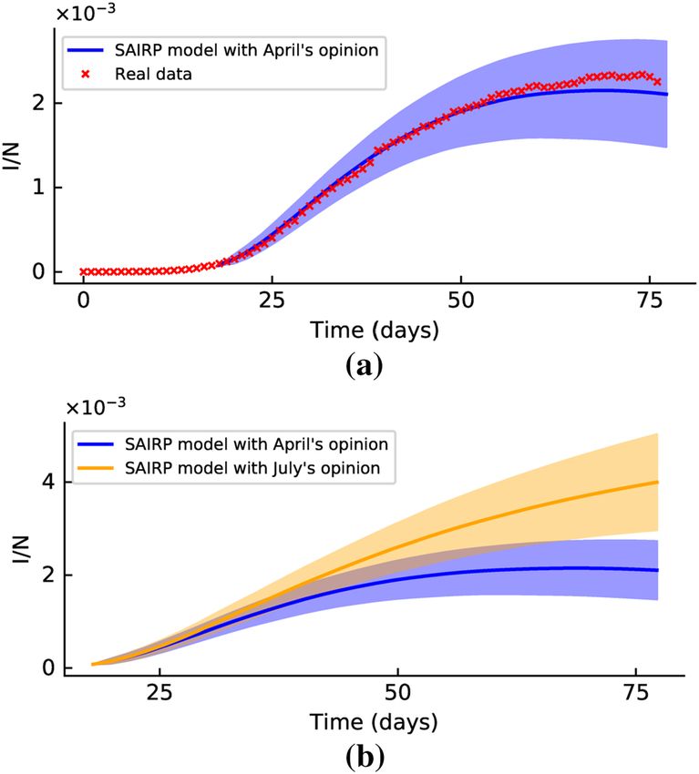
The results of the SAIRP model with the opinion distributions included are presented in Fig. 3a. The red
crosses mark the experimental observations until May 17 and the blue line is the fit to the SAIRP model with the
opinion distribution. The model simulation was repeated 12000 times in order to gain statistical significance,
i.e., the evolution of the number of infected individuals shown in Fig. 3 is consistent and does not depend on a
limited number of realizations, but is rather generic as the average over a significantly large number of simula-
tions. The parameters used for these simulations are in Table 4, in the “Methods” section.
In Fig. 3b, the results of the SAIRP model, coupled with the opinion distributions, are shown for the two situ-
ations considered. The blue line corresponds to the situation in April 2020. The yellow line shows a possible line
of evolution of the pandemic in case the distribution of opinion is such as in July 2020 (the rest of the parameters
Scientific Reports | (2021) 11:3451 | https://doi.org/10.1038/s41598-021-83075-6 4
Vol:.(1234567890)www.nature.com/scientificreports/
Figure 3. Evolution of the number of infected individuals (normalized by the total population) with time. (a)
Red crosses correspond to the experimental recordings while the blue line is the fit of the SAIRP model with
opinion. The bluish shadow marks the uncertainty of the model. (b) Blue line is the fit of the SAIRP model
coupled with the opinion distribution, corresponding to April 2020, and the yellow line is the evolution of the
model coupled with the state of social opinion as in July 2020.
were kept as in the blue curve). Note that the yellow line shows a much worse scenario and it is a direct conclu-
sion of a change in the distribution of opinions.
Optimal control. We obtain optimal control strategies that respect the following important constraints. (i)
One needs to ensure that the number of hospitalized individuals with COVID-19 is such that the health system
can respond to the other diseases in the population, in order that the mortality associated with other causes does
not increase. (ii) It is important that the number of active infected individuals is always below a critical level.
(iii) In order to keep the country “working”, there is always a percentage of the population that is susceptible to
get infected. For instance, it is very important to keep schools open, in particular for children under 10/12 years
old; there are always people that do not follow the rules imposed by the government; etc. Roughly speaking,
our goal is to maximize the number of people that go back to “normal life” and minimize the number of active
infected (and, consequently, the number of hospitalized and in ICUs), ensuring that the health system is never
overloaded.
Hospitals and intensive care units occupancy beds by COVID‑19. For the hospitalized individuals, the official
data for the fraction of hospitalized individuals due to COVID-19, represented by H, with respect to the active
infected individuals I is plotted in Supplementary Fig. 2 (a), H/I. We observe that after a first period, where all the
active confirmed cases were hospitalized, the so-called containment phase, the percentage of active infected indi-
viduals that needs hospital treatment is always below 15%. Moreover, after the end of the emergency states (red
dot in Supplementary Fig. 2), the percentage of active infected individuals that needs to be treated at hospitals is
less or equal than 5% (the 15% and 5% are plotted with dotted blue lines in Supplementary Fig. 2).
For the percentage of active infected individuals that need to be in intensive care units (ICU), we observe
that (see Supplementary Fig. 2 (b)) the proportion of active infected individuals that requires medical assistance
in ICU is always below than 6% and, moreover, after the end of the state of emergency the percentage of active
infected individuals in the ICU is always below 1%.
Introduction of the control and its optimization. One of the main challenges, facing countries struck by the
pandemic, is the reopening of the economy while preserving the health of the population without collapsing
the public health system. It is very important to keep the schools open (remember that children under 10/12
years old are not obliged to use a mask in Portugal) and prevent the economy to sink. Thus, there is a minimum
number of people that need to be susceptible to infection. But we also need to account that the population do
not always follow the rules imposed by governments. We have developed tools to quantify this effect and include
it into the equations. With this idea in mind, we investigate the use of optimal control theory to design strate-
Scientific Reports | (2021) 11:3451 | https://doi.org/10.1038/s41598-021-83075-6 5
Vol.:(0123456789)www.nature.com/scientificreports/
gies for this phase of the disease. The goal now is to maximize the number of people transferred from class P to
the class S (that helps keeping the economy alive) and, simultaneously, minimize the number of active infected
individuals and, consequently, the number of hospitalized and people needing ICU (in other words, ensuring
that the health system is never overloaded). We want to impose that the number of active infected cases is always
below 2/3 or 60% of the maximum value observed up to now ( Imax ). This condition warrants that the health
system does not collapse.
The fraction of protected individuals P that is transferred to susceptible S, is mathematically represented, in
the SAIRP model, by the parameter m. The class of active infected individuals I is very sensitive to the change of
the parameter m (Supplementary Fig. 3).
Taking into consideration the real official data of COVID-19 in P ortugal21, let Imax = 2.5 × 10⁻³ represent
the maximum fraction of active infected cases observed in Portugal from March 2, 2020 until July 29, 2020. Note
that for m 0.25 the constraint I(t) 0.75 × Imax is not satisfied for the uncontrolled model (1). This means that
the need of hospital beds and ICU beds can take vales such that the Health System can not respond, so we take
the maximum value Imax as a reference point for the state constraints imposed on the optimal control problem,
in order to ensure that in a future second epidemic wave the number of active infected cases remains below a
certain percentage of this observed maximum value.
The parameter m in the SAIRP model, is replaced by a control function u(·). We formulate mathematically
this optimal control problem and solve it (see “Methods”).
The control function u takes values between 0 and umax , with umax 1. When the control u takes the value 0
there is no transfer of individuals from P to the class S; when u takes the value umax , then umax % of individuals
in the class P are transferred to the class S at a rate w (see Table 2 in “Methods” for the meaning of parameter w).
We consider a time window of 120 days. In the Supplementary Information, we analyze with more detail
the optimal control problem subject to I 2/3 × Imax and umax 0.95 (see Supplementary Figs. 4–6 and Sup-
plementary Table 1).
Remark The optimal control problem under the state constraint I 2/3 × Imax is associated with a solution that
implies a substantial and important difference on the number of hospital beds occupancy and in intensive care
units with respect to the optimal control problem subject to the state constraint I 0.60 × Imax . The choice of
the constraints I 2/3 × Imax and I 0.60 × Imax comes from the mathematical numerical simulations carried
out and the number of hospitals beds that the Portuguese Health System has available for COVID-19 assistance.
The controlled solution takes the maximum value umax in a first period of time, followed by a period where
there are no transfer of individuals from the class P to the class S and, at the final period of time, it takes the
maximum value again (Fig. 4a,b). The case umax > 0.5 corresponds to a large number of days where there is no
transfer of individuals from the class P to S (Fig. 4c,d and Supplementary Fig. 5).
The time with no transfer from P to S corresponds to a window of time where strict rules are imposed to the
population, that can include home confinement, for example. This interval of time increases when the maxi-
mum value of the control umax increases (see Supplementary Figs. 7 and 8). We are able to compute the absolute
number of individuals that are released to the class S in terms of umax , which is a strictly increasing function of
time (see Supplementary Fig. 9).
Without loss of generality, in what follows we consider 0 < umax 0.25 , and analyze the hospital bed
occupancy and ICU beds, due to COVID-19, associated to the optimal solutions that satisfy the constraint
I 0.60 × Imax (see Fig. 5). For the bed occupancy due to COVID-19, we give information about the number
of total beds needed in the cases where the percentage of active infected individuals that needs hospital care was
between 5% and 15% (see Fig. 5a). This number is relatively small for the Portuguese capacities and will allow
the medical assistance for non COVID-19 diseases.
Considering a range of values for maximum value of the percentage of protected individuals that is trans-
ferred to the susceptible between 0.05 and 0.25, that is umax ∈ {0.05, 0.10, 0.15, 0.20, 0.25}, the number of hospital
beds needed to treat COVID-19 patients have a variation of 1448 beds, in the case when 15% of active infected
individuals need medical assistance (see Fig. 5b). For the ICU bed occupancy, in the case where 3% of the active
infected individuals require to be in ICU, the number of beds is presented in Fig. 5c and it may differ of 290 beds,
when umax varies from 0.05 to 0.25.
Discussion
Portugal is a country that felt naturally isolated during most of the quarantine, so the data were not disturbed by
spurious influences from other countries. Moreover, the disease was quite controlled at all times, the distribu-
tion of the population, as well as the distribution of social classes, is quite homogeneous countrywide and, thus,
mathematical models are better suited to an analysis in a country like Portugal. Since the society behaves quite
homogeneously across the country, we claim the social analysis here included to be quite relevant. To the best of
our knowledge, this is the first work to investigate the reality of COVID-19 in Portugal and suggesting control
measures coming from the mathematical theory of optimal control.
Optimal control theory is a branch of mathematics that offers a tool to tackle the problem of finding optimal
strategies to stop the transmission of SARS-CoV-2. It is a powerful tool to design control strategies and act opti-
mally on a given system. Based on reliable mathematical models for transmission mechanism of COVID-19,
mathematical optimal control can thus help and assist the Public Health Authorities to understand, anticipate
and mitigate the spread of the virus, and evaluate the potential effectiveness of specific prevention strategies.
A compartmental deterministic model describing the course of the epidemic, using data from Italy during the
first 46 days (from February 20 through April 5, 2020), concluded that “restrictive social-distancing measures will
Scientific Reports | (2021) 11:3451 | https://doi.org/10.1038/s41598-021-83075-6 6
Vol:.(1234567890)www.nature.com/scientificreports/
10-3 I/N subject to Iwww.nature.com/scientificreports/
(a)
Hospital bed occupancy
4000 u max =0.05
u max =0.10
u max =0.15
3000
Number of beds
u max =0.20
Difference of 1 448 beds u max =0.25
2000
15% of active infected
1000
Difference of 483 beds 5% of active infected
0
0 20 40 60 80 100 120
Time (days)
(b)
ICU - Bed occupancy
u max =0.05
800 u max =0.10
u max =0.15
Number of beds
600 u max =0.20
Difference of 290 beds u max =0.25
400
Difference of 145 beds 3% of active infected
200
1.5% of active infected
0
0 20 40 60 80 100 120
Time (days)
(c)
Figure 5. Number of hospital beds occupation for the optimal control solutions. (a) Number of hospital
beds for umax ∈ {0.05, 0.10, 0.15, 0.20} subject to I(t) 0.60 × Imax varying between 5% and 15% of the
number of infected individuals. (b) Number of hospital beds for umax ∈ {0.05, 0.10, 0.15, 0.20, 0.25} under
the state constraint I(t) 0.60 × Imax , representing between 5% and 15% of the number of active infected
individuals. (c) ICU hospital bed occupancy for umax ∈ {0.05, 0.10, 0.15, 0.20, 0.25} under the state constraint
I(t) 0.60 × Imax . The ICU beds occupation represents between 1.5% and 3% of the number of active infected
individuals.
In many countries, Portugal included, the so-called non-pharmaceutical interventions (NPIs) were taken
since the first confirmed case. Therefore, our mathematical model considers a class of individuals that practice,
in an effective way, the NPIs measures and, therefore, is protected from the virus. Based on recent s tudies19,20, we
assume that the individuals that follow NPIs measures are protected from infection of SARS-CoV-2. It is impor-
tant to keep people in the class of protected/prevented due to the existing risk of transmission of the infection
by asymptomatic infected i ndividuals25.
We propose a SAIRP mathematical model, that represents the transmission dynamics of SARS-CoV-2 in a
homogeneously mixing constant population. The SAIRP model fits the confirmed active infected individuals in
Portugal, from the first confirmed case, on March 2, 2020, until July 29, 2020, using real data from Portuguese
Scientific Reports | (2021) 11:3451 | https://doi.org/10.1038/s41598-021-83075-6 8
Vol:.(1234567890)www.nature.com/scientificreports/
Population compartment Description
S Susceptible
A Asymptomatic
I Confirmed/active infected
R Recovered/removed (includes deaths by COVID-19)
P Protected/prevented
Table 1. Description of the population model compartments.
National Authorities21. The new model considers a class of individuals that we call protected/prevented, repre-
senting the fraction of individuals that is under effective protective measures, preventing the spread of SARS-
CoV-2. In a first phase, from March 14 until May 02, 2020, this class represented all the individuals that were in
confinement, due to closed schools, layoff, etc. After the three states of emergency implemented in Portugal, the
confinement measures started to be raised but, simultaneously, other prevention measures were recommended
by the Government, such as the use of mask, that became mandatory in closed spaces. All the individuals that
practice, in a effective way, all NPIs, are considered to belong to class P. The social opinion network implemented
shows how the Portuguese population has followed the health authorities policies and recommendations: social
distance, use of mask, avoid of celebrations, etc. In practice, this can be related to the partial maintenance of the
population in the class P of the SAIRP model. However, there is always a significant percentage of the popula-
tion that does not follow, in an effective way, the official recommendations. Moreover, there are groups in the
population that are crucial to a “normal life” and cannot avoid close physical and unprotected contacts, such as
children in kindergartens and primary schools. With this background, we formulate an optimal control prob-
lem, where the control represents the percentage of protected/prevented individuals that are transferred to the
susceptible class, that is, is not under protective measures. The goal to consider such optimal control problem
is to find the optimal strategy to transfer individuals from protected/prevented class to the class of susceptible,
with minimal active infected individuals and always below a specific threshold that maintains the number of
hospitalized individuals due to COVID-19 and hospitalized in intensive care units, below the level that the
National Health Service is able to answer while keeping the other “usual” medical services working normally.
This is also connected with the political and social interest of keeping the economy open and “active”. We provide
the mathematical optimal control solutions for different scenarios on the fraction of protected individuals that
is transferred to the susceptible class and also for different threshold levels.
We conclude with some words explaining why we believe optimal control has an important role in helping
to prevent COVID-19 dissemination, and also pointing out some possible future research directions. In general,
the response to chronic health problems has been impaired, both because the resources were largely allocated
to COVID-19 or because the population was afraid to go to the hospitals and many surgeries and consultations
remain to be made. Many institutions have organized what has been called in Portugal “home hospitalization”,
which served to mitigate many problems that would remain unanswered. Hospital teams, multidisciplinary
teams, systematically moved to the homes of patients and sought care in their environment, avoiding nosocomial
infections and also the occupation of beds. This experience was evaluated as very positive by the Portuguese
population. Most probably, this coronavirus will remain in the communities for many years, so the changes we
see in health services and in people’s habits have to go on over time. Actions as simple as hand washing, space
hygiene, social distance and use of masks in closed spaces, should be incorporated into education for health.
The containment measures, which should be necessary when outbreaks arise, must be rigorously studied and
worked with families. Confinement cannot mean social isolation and should be worked out according to each
family reality. The latest data shows that European countries are already at the limit in terms of reinforcements
to NHS budgets. Changing many hospital practices, such as cleanliness and hygiene, food services, relationship
between emergencies and hospitalization, support for clinical training of health professionals, etc., can help to
rationalize resources and prevent infections to other users, especially in autumn and winter, where different
forms of flu and pneumonia burden institutions. At this moment we do not include such “social” corrections in
the optimal control part, but it would be interesting to consider them in future work.
Methods
Mathematical epidemiological model. The SAIRP model (1) subdivides human population into five
mutually-exclusive compartments (see Table 1 and Supplementary Fig. 1), representing the dynamical evolution
of the population in each compartment over a fixed interval of time.
The susceptible individuals become infected by SARS-CoV-2 by contact with infected asymptomatic A and
active infected individuals I. The rate of infection is given by β(θA(t) + I(t)), where β is the infection transmis-
sion rate of active infected individuals I and θ represents a modification parameter for the infectiousness of the
asymptomatic infected individuals (A). A fraction p, with 0 < p < 1, is protected from infection by SARS-CoV-2,
due to an effective implementation of non-pharmaceutical interventions (NPIs) and is transferred to the class
P, at a rate φ . However, individuals in the class P are not immune to infection and a fraction m can become
susceptible again at a rate w. For the sake of simplification, we denote ω = wm. A fraction q of asymptomatic
infected individuals A develop symptoms and are detected, at a rate v, being transferred to the class I. We use the
notation ν = vq. Active infected individuals I exit this class either by recovery from the disease or by COVID-19
induced death, being transferred to the class of removed/recovery R, at a rate δ (see Table 2).
Scientific Reports | (2021) 11:3451 | https://doi.org/10.1038/s41598-021-83075-6 9
Vol.:(0123456789)www.nature.com/scientificreports/
Parameter/ Description
β Infection transmission rate
θ Modification parameter
p Fraction of susceptible S transferred to protected class P
φ Transition rate of susceptible S to protected class P
ω = wm
w Transition rate of protected P to susceptible S
m Fraction of protected P transferred to susceptible S
ν = vq
v Transition rate of asymptomatic A to active/confirmed infected I
q Fraction of asymptomatic A infected individuals
δ Transition rate from active/confirmed infected I to removed/recovered R
Table 2. Description of the parameters of model (1).
The previous assumptions are described by the following system of five ordinary differential equations:
Ṡ(t) = −β(1 − p)(θ A(t) + I(t))S(t) − φpS(t) + ωP(t),
Ȧ(t) = β(1 − p)(θA(t) + I(t))S(t) − νA(t),
İ(t) = νA(t) − δI(t), (1)
Ṙ(t) = δI(t),
Ṗ(t) = φpS(t) − ωP(t).
Remark The testing rate in Portugal, as in many other countries, has been increasing since the beginning of the
pandemic. However, in our model we do not consider the impact of the testing rate on the detection of infected
cases. This is due to the fact that in Portugal only suspected individuals that had a close contact, without mask
protection, or individuals with COVID-19 symptoms, are tested.
Remark In our model (1), individuals from compartment A move to compartment I. Given testing frequencies
and reliability, we adjust the infection rate and consider a proportion of detection. The parameter q is used to
obtain the proportion of A moving to I. In a general framework, a fraction (1 − q) of asymptomatic individuals
A should be transferred to the compartment R. However, in this work we are based on the official data provided
by The Portuguese Health Authorities and our aim is to propose a mathematical model that fits well the reality
described by the daily reports data, more specifically the curve of the active infected individuals by COVID-19
in Portugal and, sub-sequentially, the fraction of active individuals that are hospitalized and in intensive care
units. Using official data, only the individuals that were confirmed to be infected by testing (the ones that are
represented by the class I) may be transferred to the class R. Therefore, since the asymptomatic are not counted
in the official data, it is not possible (in this model) to count them as recovered after a certain number of days.
Let us define the total population N by N(t) = S(t) + A(t) + I(t) + R(t) + P(t). Taking the derivative of
N(t), it follows from (1) that Ṅ(t) = 0, that is, N is constant over time. Without loss of generality, we normalize
the system so that N = 1. All parameters of the model are non-negative and, given non-negative initial condi-
tions (S0 , A0 , I0 , R0 , P0 ) = (S(0), A(0), I(0), R(0), P(0)), the solutions of system (1) are non-negative and satisfy
S(t) + A(t) + I(t) + R(t) + P(t) = 1 for all time t ∈ [0, tf ]. With this conservation law, the model (1) can be
simplified to 4 equations, the cumulative number of removed/recovered individuals R(t) being given, for each
t 0, by
t
R(t) = R(0) + δ I(s) ds . (2)
0
Therefore, we consider the following SAIP simplified model for the optimal control problem formulation:
Ṡ(t) = −β(1 − p)(θ A(t) + I(t))S(t) − φpS(t) + ωP(t),
Ȧ(t) = β(1 − p)(θA(t) + I(t))S(t) − νA(t),
İ(t) = νA(t) − δI(t), (3)
Ṗ(t) = φpS(t) − ωP(t).
Remark In our model we are taking into account the infectiousness of fully asymptomatic patients A. In concrete,
the transmission incidence is given by the term β(1 − p)(θA(t) + I(t)).
The disease free equilibrium 0 of model (3) is given by
Scientific Reports | (2021) 11:3451 | https://doi.org/10.1038/s41598-021-83075-6 10
Vol:.(1234567890)www.nature.com/scientificreports/
ω φp
�0 = S= , A = 0, I = 0, P = (4)
φp+ω φp+ω
with S + P = 1. Following the approach of Driessche and Watmough26, the basic reproduction number R0 is
given by the spectral radius of FV −1, where the matrices F, V and FV −1 are given by
−Sβ(p − 1)θ − β(p − 1)S ν 0
F= , V= ,
0 0 −ν δ
β(p−1)θ ω β(p−1)ω β(p−1)ω
− (φp+ω)ν − (φp+ω)δ − (φp+ω)δ
FV −1 = ,
0 0
that is,
β(1 − p) ω (θδ + ν)
R0 = . (5)
(φp + ω) ν δ
Parameter values and estimation from Portuguese COVID‑19 data. We consider official data,
where daily reports are available with the information about total (cumulative) confirmed infected cases, total
recovered, and total deaths by COVID-19 in Portugal, and also information about the number of hospitalized
individuals and in intensive care due to COVID-19 disease21.
We assume θ = 1 for the current (up to the date) best estimate for the infectiousness of asymptomatic individ-
uals relative to symptomatic i ndividuals27. For the fraction of asymptomatic A infected individuals, we consider
q = 0.1528–30. The parameter w takes the value w = 1/45 day −1, corresponding to the 3 emergency states (duration
45 days)22. The value of the parameter δ, representing the recovery time of confirmed active infected individu-
als I(t) (with negative test)/removed (by death), is assumed to be δ = 1/30 days−1, considering that here might
be a delay on the publication of real data31. The parameters β1, β3, m1 and m3 were estimated using the Matlab
function lsqcurvefit for t ∈ [100, 150] days, respectively. From March 2 to May 17, 2020 (77 days): t ∈ [0, 77]
– β1 = 1.492, m1 = 0.059, and p1 = 0.675. From May 17 to June 9, 2020 (23 days): t ∈ [77, 100] – β2 = 0.25,
m2 = 0.058 and p2 = 0.4 . From June 9 to July 29, 2020 (50 days): t ∈ [100, 150] – β3 = 1.91, m3 = 0.043, and
p3 = 0.4 . The fraction 0 < p1 < 1, for t ∈ [0, 77], is assumed to take the value p1 = 0, 675, representing the
population affected by the confinement of policies21,22. For t ∈ [77, 100], we assume a decrease of the fraction
of protected individuals to p2 = 0.55. For t ∈ [100, 150], we assume p3 = 0.44 , based on a gradual transfer of
individuals from the class P to the class S. The transfer of individuals from S to P started on March 14, 202022,32,
thus we take φ = 1/12 day −1.
Building the social network. In order to generate the social network, we use data collected from the
micro-blogging website Twitter. With aid of the Python package GetOldTweets333, we were able to download
a collection of several tweets (posts of 244 characters) attending to participation in a given hashtag. Merging a
handful of different hashtags, we obtained a significant sample of users who are interacting between themselves,
either exchanging information with replies or spreading it via what is called a “re-tweet”. The more hashtags we
use, the more realistic is the reconstruction of the social network in regards to the actual situation of the Portugal
Twitter network. In mathematical terms, we build a complex neiork where users lie in the nodes and the directed
edges represent the interactions between users. We are mainly interested on the structure of the interactions
rather than the topic of the information, and thus we discard everything related to the personal information of
the users and the content of the tweets.
Most real world networks are changing in time, either by changes on the connectivity pattern or either by
growth and continuous addition of new nodes. This is a key feature of the so called scale-free complex n etwork35,
and it is a feature shared by the social network Twitter36–38. Thus, the structure of the network can drastically
change from one month to another, and so it is important to take this point into account when building the
network. In our data, this was accomplished by a feature of the used package, which allows to filter the search
by date. In fact, here we were also interested in comparing the behavior of the social network during April,
when the quarantine was imposed, and the social network during July, when the social distancing measures
relaxed. The connectivity distributions for both networks are shown in Supplementary Fig. 10. In both cases,
the topology corresponds with that of a scale free network but with rather different exponents, γApril = 2.11 and
γJuly = 1.82. The significantly different exponents demonstrate the different internal dynamics in both cases,
which are reflected in the opinion distributions.
Opinion model. The network topology obtained was endowed with a dynamical opinion set of equations
for each node (actual person) that, combined with the information coming through the network connections,
allowed it to produce an opinion. We considered a simple opinion model based on the logistic e quation39 but that
has proved to be of use in other contexts40–42. The equations describing each node i, i = 1, . . . , N , are42:
N
dui 1
= f (ui ) + d Lij uj , (6)
dt ki
j=1
Scientific Reports | (2021) 11:3451 | https://doi.org/10.1038/s41598-021-83075-6 11
Vol.:(0123456789)www.nature.com/scientificreports/
where ui is the opinion of node i that ranges from zero to one. The nonlinearity f (ui ) is given by the following
equation:
(7)
f (u) = u A(1 − u/B) + g(1 − u) .
Each of the nodes i obeys the internal dynamic given by f (ui ) while being coupled with the rest of the nodes
with a strength d/ki , where d is a diffusive constant and ki is the connectivity degree for node i (number of nodes
each node is interacting with). Note that this is a directed non-symmetrical network where ki means that node i is
following the tweets from ki nodes and, thus, it is being influenced by those nodes in its final opinion. The Lapla-
cian matrix Lij is the operator for the diffusion in the discrete space, i = 1, . . . , N . We can obtain the Laplacian
matrix from the connections established within the network as Lij = Aij − δij ki , being Aij the adjacency matrix:
1 if i, j are connected,
Aij =
0 if i, j are not connected. (8)
Now, we proceeded as follows. We considered that all the accounts (nodes in our network) were in their stable
fixed point with a 10% of random noise. Then a subset of the nodes was forced to acquire a different opinion,
ui = 1 with a 10% of random noise and we let the system to evolve following the above dynamical equations. The
influence of the network made some of the nodes to shift their opinion to values closer to 1 that, in the context
of this simplified opinion model, means that those nodes shifted their opinion to values closer to those leading
the shift in opinion. This process was repeated in order to gain statistical significance and, as a result, it provided
the probability distribution of nodes eager to change the opinion and adhere to the new politics. The parameter
values used were A = 0.00001, B = 0.1, g = 0.001 and d = 1.0.
Parameter values for the SAIRP model with opinion distributions. The parameters used and the
initial conditions are summarized in Table 4. Once the opinion distribution was included into the SAIRP model,
the parameters were slightly adjusted to be able to continue describing accurately the experimental situation. In
fact, moving from an only-time-dependent-model to the network type model we consider in this section implies
that the whole dynamic of the system is speeded up as now each node has the capability to trigger the epidemic
wave. In order to compensate this effect, a rescaling of the parameters controlling the temporal scale in the sys-
tem, namely δ, φ and w, is necessary. An estimated rescaling factor of 1.85 leaves the modified parameters shown
in Table 4. With the opinion distribution included into the SAIRP model, the infection transmission rate also
needs to be adjusted in order to continue describing accurately the experimental situation.
Optimal control problem. The goal is to find the optimal strategy for letting people to go out from class
P to the class S and, at the same time, minimize the number of active infected while keeping the class of active
infected individuals below a safe maximum value.
The control u(·) represents the fraction of individuals in class P of protected that is transferred to the class S.
The control u is introduced into the SAIP model in the following way:
Ṡ(t) = −β(1 − p)(θ A(t) + I(t))S(t) − φpS(t) + wu(t)P(t),
Ȧ(t) = β(1 − p)(θA(t) + I(t))S(t) − νA(t),
(9)
İ(t) = νA(t) − δI(t),
Ṗ(t) = φpS(t) − wu(t)P(t).
The control must satisfy the following constraints: 0 u(t) umax with umax 1. In other words, the solu-
tions of the problem must belong to the following set of admissible control functions:
� = u, u ∈ L1 [0, tf ], R | 0 u(t) umax ∀ t ∈ [0, tf ] . (10)
Mathematically, the main goal consists to minimize the cost functional
tf
J(u) = k1 I(t) − k2 u(t) dt , (11)
0
representing the fact that we want to minimize the fraction of infected individuals I and, simultaneously, maxi-
mize the intensity of letting people from class P go back to class S. The constants ki, i = 1, 2, represent the weights
associated to the class I and control u. Moreover, the solutions of the optimal control problem must satisfy the
following state constraints: I(t) ζ with ζ = 0.6 × Imax and ζ = 2/3 × Imax.
For the numerical simulations, we considered k1 = 100 , k2 = 1 and tf = 120 days. We also considered
(β, δ) = (1.464, 1/30), m = 0.09, p = 0.675, and all the other parameters from Table 3. Numerically, we discre-
tized the optimal control problem to a nonlinear programming problem, using the Applied Modeling Program-
ming Language (AMPL)43. After that, the AMPL problem was linked to the optimization solver IPOPT44,45. The
discretization was performed with n = 1500 grid points using the trapezoidal rule as the integration method.
Scientific Reports | (2021) 11:3451 | https://doi.org/10.1038/s41598-021-83075-6 12
Vol:.(1234567890)www.nature.com/scientificreports/
Parameter/Initial condition Value Reference
β1 1.492 Estimated
β2 0.25 Estimated
β3 1.91 Estimated
27
θ 1
21,22
p1 0.675
p2 0.55
p3 0.40
22,32
φ 1/12 day −1
ω = wm
w 1/45 day −1 22
m1 0.059 Estimated
m2 0.058 Estimated
m3 0.043 Estimated
ν = vq
v 1 day −1
q 0.15 28–30
31
δ 1/30 day −1
34
N = S0 + A0 + I0 + R0 + P0 10295909
21
S0 10295894/N
21
I0 2/N
21
A0 (2/0.15)/N
21
R0 0
21
P0 0
Table 3. Initial conditions and parameter values for Portugal from March 2, 2020 to June 19, 2020. Contrast
with Fig. 1. The parameters β1, β2 and β3, and m1, m2 and m3 were estimated using the Matlab function
lsqcurvefit for t ∈ [0, 77] and t ∈ [100, 150] days, respectively. From March 2 to May 17, 2020 (77 days):
t ∈ [0, 77] – β1 = 1.492, m1 = 0.059 and p1 = 0.675. From May 17 to June 9, 2020 (23 days): t ∈ [77, 100]
– β2 = 0.25, m2 = 0.058 and p2 = 0.4. From June 9 to July 29, 2020 (50 days): t ∈ [100, 150] – β3 = 1.91,
m3 = 0.043 and p3 = 0.4.
Parameter/Initial condition Value
β 0.2
φ 1/6.486 day −1
w 1/24.32 day −1
v 1 day −1
q 0.15
δ 1/16.216 day −1
N = S0 + A0 + I0 + R0 + P0 25000
S0 (N − 2 − 2/0.15)/N
I0 2/N
A0 (2/0.15)/N
R0 0
P0 0
Table 4. Initial conditions and parameter values for Portugal from March 2, 2020 to May 17, 2020 for the
SAIRP model, modified by the opinion distributions.
Data availability
All of the data are publicly available and were extracted from https: //covid1 9.min-saude. pt/relato
rio-de-situac ao/.
Code availability
The code is available from the authors on request.
Scientific Reports | (2021) 11:3451 | https://doi.org/10.1038/s41598-021-83075-6 13
Vol.:(0123456789)www.nature.com/scientificreports/
Received: 6 October 2020; Accepted: 27 January 2021
References
1. Peeri, N. C. et al. The SARS, MERS and novel coronavirus (COVID-19) epidemics, the newest and biggest global health threats:
What lessons have we learned?. Int. J. Epidemiol. 49, 717–726 (2020).
2. COVID-19 Coronavirus Pandemic. https://www.worldometers.info/coronavirus/ (2020).
3. República Portuguesa, Ministério da Educação, XXII Governo. Comunicação enviada às escolas sobre suspensão das atividades
com alunos nas escolas de 16 de março a 13 de abril. https://www.portugal.gov.pt/pt/gc22/comunicacao/documento?i=comunicaca
o-enviada-as-escolas-sobre-suspensao-das-atividades-com-alunos-nas-escolas-de-16-de-marco-a-13-de-abril (2020).
4. Capacidade de Medicina Intensiva aumentou 23%. https: //covid1 9.min-saude. pt/capaci dade- de-medici na-intens iva-aument ou-23/
(2020).
5. Metcalf, C. J. E., Morris, D. H. & Park, S. W. Mathematical models to guide pandemic response. Science 369, 368–369 (2020).
6. Giordano, G. et al. Modelling the COVID-19 epidemic and implementation of population-wide interventions in Italy. Nat. Med.
26, 855–860 (2020).
7. López, L. & Rodó, X. The end of social confinement and COVID-19 re-emergence risk. Nat. Hum. Behav. 4, 746–755 (2020).
8. Hoertel, N. et al. A stochastic agent-based model of the SARS-CoV-2 epidemic in France. Nat. Med. 26, 1801 (2020).
9. Kissler, S. M., Tedijanto, C., Goldstein, E., Grad, Y. H. & Lipsitch, M. Projecting the transmission dynamics of SARS-CoV-2 through
the postpandemic period. Science 368, 860–868 (2020).
10. Campos, C., Silva, C. J. & Torres, D. F. M. Numerical optimal control of HIV transmission in Octave/MATLAB. Math. Comput.
Appl. 25(1), 20 (2020).
11. Malinzi, J., Ouifki, R., Eladdadi, A., Torres, D. F. M. & White, K. A. J. Enhancement of chemotherapy using oncolytic virotherapy:
Mathematical and optimal control analysis. Math. Biosci. Eng. 15(6), 1435–1463 (2018).
12. Sharomi, O. & Malik, T. Optimal control in epidemiology. Ann. Oper. Res. 251(1–2), 55–71 (2017).
13. Rawson, T., Brewer, T., Veltcheva, D., Huntingford, C. & Bonsall, M. B. How and when to end the COVID-19 lockdown: An
optimization approach. Front. Public Health 8, 262 (2020).
14. Tsay, C. et al. Modeling, state estimation, and optimal control for the US COVID-19 outbreak. Sci. Rep. 10, 10711 (2020).
15. Libotte, G. B., Lobato, F. S., Platt, G. M. & Neto, A. J. S. Determination of an optimal control strategy for vaccine administration
in COVID-19 pandemic treatment. Comput. Methods Programs Biomed. 196, 105664 (2020).
16. Obsu, L. L. & Balcha, S. F. Optimal control strategies for the transmission risk of COVID-19. J. Biol. Dyn. 14, 590–607 (2020).
17. Zine, H. et al. stochastic time-delayed model for the effectiveness of Moroccan COVID-19 deconfinement strategy. Math. Model.
Nat. Phenom. 15, 14 (2020) (Art. 50).
18. Moradian, N. et al. The urgent need for integrated science to fight COVID-19 pandemic and beyond. J. Transl. Med. 18, 205 (2020).
19. Chu, D. K. et al. Physical distancing, face masks, and eye protection to prevent person-to-person transmission of SARS-CoV-2
and COVID-19: A systematic review and meta-analysis. Lancet 395, 1973–1987 (2020).
20. Haug, N. et al. Ranking the effectiveness of worldwide COVID-19 government interventions. Nat. Hum. Behav. 4, 1303–1312
(2020).
21. Direção-Geral da Saúde—COVID-19, Ponto de Situação Atual em Portugal. https: //covid1 9.min-saude. pt/ponto- de-situac ao-atual
-em-portugal/ (2020).
22. Legislação Compilada—COVID-19. https://dre.pt/legislacao-covid-19-upo (2020).
23. Watts, D. J. & Strogatz, S. H. Collective dynamics of small-world networks. Nature 393, 440–442 (1998).
24. Teslya, A. et al. Impact of self-imposed prevention measures and short-term government-imposed social distancing on mitigating
and delaying a COVID-19 epidemic: A modelling study. PLoS Med. 17(7), e1003166 (2020).
25. Moghadas, S. M. et al. The implications of silent transmission for the control of COVID-19 outbreaks. Proc. Natl. Acad. Sci. U.S.A.
117, 17513–17515 (2020).
26. van den Driessche, P. & Watmough, J. Reproduction numbers and sub-threshold endemic equilibria for compartmental models
of disease transmission. Math. Biosci. 180, 29–48 (2002).
27. COVID-19 Pandemic Planning Scenarios. https://www.cdc.gov/coronavirus/2019-ncov/hcp/planning-scenarios.html (2020).
28. Li, R. et al. Substantial undocumented infection facilitates the rapid dissemination of novel coronavirus (SARS-CoV-2). Science
368, 489–493 (2020).
29. Mizumoto, K., Kagaya, K., Zarebski, A. & Chowell, G. Estimating the asymptomatic proportion of coronavirus disease 2019
(COVID-19) cases on board the Diamond Princess cruise ship, Yokohama, Japan, 2020. Euro Surveill. 25(10), 2000180 (2020).
30. Park, S. W., Cornforth, D. M., Dushoff, J. & Weitz, J. S. The time scale of asymptomatic transmission affects estimates of epidemic
potential in the COVID-19 outbreak. Epidemics 31, 100392 (2020).
31. Bi, Q. et al. Epidemiology and transmission of COVID-19 in 391 cases and 1286 of their close contacts in Shenzhen, China: a
retrospective cohort study. Lancet Infect. Dis. 20, 911–919 (2020).
32. Lemos-Paião, A. P., Silva, C. J. & Torres, D. F. M. A new compartmental epidemiological model for COVID-19 with a case study
of Portugal. Ecol. Complex. 44, 100885 (2020).
33. Python package GetOldTweets3. https://pypi.org/project/GetOldTweets3/
34. Statistics Portugal. https://www.ine.pt/xportal/xmain?xpid=INE&xpgid=ine_indicadores&contecto=pi&indOcorrCod=00082
73&selTab=tab0 (2020).
35. Albert, R. & Barabasi, A.-L. Statistical mechanics of complex networks. Rev. Mod. Phys. 74, 47 (2002).
36. Pereira, F. S., de Amo, S. & Gama, J. Evolving centralities in temporal graphs: A twitter network analysis. 17th IEEE International
Conference on Mobile Data Management (MDM) 2, 43–48 (2016).
37. Abel, F., Gao, Q., Houben, G. J. & Tao, K. Analyzing temporal dynamics in twitter profiles for personalized recommendations in
the social web. Proceedings of the 3rd International Web Science Conference, 1–8 (2011).
38. Cataldi, M., Di Caro, L. & Schifanella, C. Emerging topic detection on twitter based on temporal and social terms evaluation.
Proceedings of the tenth international workshop on multimedia data mining 1–10 (2010).
39. Verhulst, P. F. Resherches mathematiques sur la loi d’accroissement de la population. Nouveaux memoires de l’academie royale des
sciences 18, 1–41 (1845) ((in French)).
40. Lloyd, A. L. The coupled logistic map: A simple model for the effects of spatial heterogeneity on population dynamics. J. Theor.
Biol. 173, 217–230 (1995).
41. Tarasova, V. V. & Tarasov, V. E. Logistic map with memory from economic model. Chaos Solitons Fractals 95, 84–91 (2017).
42. Carballosa, A., Mussa-Juane, M. & Muñuzuri, A.P. Incorporating social opinion in the evolution of an epidemic spread. Submitted
(2020). Preprint at arXiv:2007.04619
43. Fourer, R., Gay, D. M. & Kernighan, B. W. AMPL: A Modeling Language for Mathematical Programming (Duxbury Press, BrooksCole
Publishing Company, 1993).
44. Wächter, A. & Biegler, L. T. On the implementation of an interior-point filter line-search algorithm for large-scale nonlinear
programming. Math. Program. 106, 25–57 (2006).
Scientific Reports | (2021) 11:3451 | https://doi.org/10.1038/s41598-021-83075-6 14
Vol:.(1234567890)You can also read