Global hydro-climatic biomes identified via multitask learning - GMD
←
→
Page content transcription
If your browser does not render page correctly, please read the page content below
Geosci. Model Dev., 11, 4139–4153, 2018
https://doi.org/10.5194/gmd-11-4139-2018
© Author(s) 2018. This work is distributed under
the Creative Commons Attribution 4.0 License.

Global hydro-climatic biomes identified via multitask learning
Christina Papagiannopoulou1 , Diego G. Miralles2 , Matthias Demuzere2 , Niko E. C. Verhoest2 , and
Willem Waegeman1
1 Department    of Data Analysis and Mathematical Modelling, Ghent University, Ghent, Belgium
2 Laboratory   of Hydrology and Water Management, Ghent University, Ghent, Belgium

Correspondence: Christina Papagiannopoulou (christina.papagiannopoulou@ugent.be)

Received: 30 March 2018 – Discussion started: 25 April 2018
Revised: 21 August 2018 – Accepted: 29 August 2018 – Published: 12 October 2018

Abstract. The most widely used global land cover and cli-        the land surface, which can be a first and necessary step to-
mate classifications are based on vegetation characteristics     wards understanding complex spatio-temporal interactions
and/or climatic conditions derived from observational data.      among different environmental variables (Feddema et al.,
However, these classification schemes do not directly stem       2005). Traditional land use and/or land cover (change) clas-
from the characteristic interaction between the local cli-       sifications are typically based on spectral information from
mate and the biotic environment. In this work, we model          the land surface coming from satellites (Loveland and Bel-
the dynamic interplay between vegetation and local climate       ward, 1997; Congalton et al., 2014). Amongst the most well
in order to delineate ecoregions that share a coherent re-       known and widely used are the International Geosphere–
sponse to hydro-climate variability. Our novel framework         Biosphere Program DISCover Global 1 km Land Cover clas-
is based on a multitask learning approach that discovers         sification (IGBP-DIS) (Loveland et al., 2000), Global Land
the spatial relationships among different locations by learn-    Cover 2000 (Bartholomé and Belward, 2005), and more re-
ing a low-dimensional representation of predictive struc-        cently the land cover map developed within the European
tures. This low-dimensional representation is combined with      Space Agency’s Climate Change Initiative (ESA CCI) (Poul-
a clustering algorithm that yields a classification of biomes    ter et al., 2015; Li et al., 2018). Similarly, climate classifica-
with coherent behaviour. Experimental results using global       tion schemes cluster regions with similar climate conditions
observation-based datasets indicate that, without the need       and are also widely used to stratify geographical regions with
to prescribe any land cover information, the identified re-      different climatic expectations (Baker et al., 2009; Brugger
gions of coherent climate–vegetation interactions agree well     and Rubel, 2013; Garcia et al., 2014; Herrando-Pérez et al.,
with the expectations derived from traditional global land       2014). Here, the best known is probably the Köppen–Geiger
cover maps. The resulting global “hydro-climatic biomes”         climate classification (Köppen, 1936), which has been mod-
can be used to analyse the anomalous behaviour of specific       ified many times in recent decades (e.g. Thornthwaite, 1943;
ecosystems in response to climate extremes and to bench-         Trewartha and Horn, 1980; Feddema, 2005; Kottek et al.,
mark climate–vegetation interactions in Earth system mod-        2006; Peel et al., 2007). Yet to date, dynamics in these cli-
els.                                                             mate regimes are used as a diagnostic of climate change
                                                                 by exploring their shifting boundaries (e.g. Diaz and Eis-
                                                                 cheid, 2007; Chen and Chen, 2013; Zhang and Yan, 2014a,
                                                                 b; Spinoni et al., 2015; Chan and Wu, 2015) or as a means
1   Introduction                                                 to predict future climatic zone distributions using climate
                                                                 projections (e.g. Hanf et al., 2012, Gallardo et al., 2013,
Approaches which aim to define regions with similar bio-         Mahlstein et al., 2013).
physical characteristics are commonly known as land cover           In recent years, the exponential advance in Earth obser-
classification schemes and are widely used in multiple geo-      vation research has made climate science one of the most
scientific disciplines. Land cover classifications are crucial   data-rich scientific domains (Faghmous and Kumar, 2014).
to enable a better understanding of the spatial variability of

Published by Copernicus Publications on behalf of the European Geosciences Union.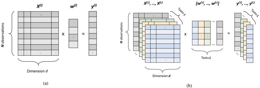
4140                           C. Papagiannopoulou et al.: Global hydro-climatic biomes identified via multitask learning

As such, data-driven methods have become popular in their          ilar interactions even if they are remotely located from each
use for land cover and climate classifications. For instance,      other. A previous effort towards detecting regions with simi-
Lund and Li (2009) proposed a new distance measure to              lar vegetation response to climate involves the work of Ivits
define seasonal means and autocorrelations of climatic time        et al. (2014), in which PCA is performed on the data matrix
series from weather stations and grouped the stations using        of drought anomalies and vegetation state, and a clustering
a hierarchical agglomerative clustering. Zscheischler et al.       is applied to the correlation coefficients based on the spatio-
(2012) also stressed the importance of unsupervised meth-          temporal patterns obtained by PCA. However, in this study,
ods for tasks such as the classification of the land surface       the interaction between climate and vegetation is not explic-
into zones with different climate and vegetation characteris-      itly learned, nor are the causes behind vegetation changes
tics. Metzger et al. (2012) applied an alternative data-driven     inferred in a predictor–target framework.
approach on climate and vegetation data that used principal           Here, we introduce for the first time (to the best of our
component analysis (PCA) to discover informative structures        knowledge) a data-driven approach that aims to quantify the
in the data. In this method, the principal components of the       response of vegetation to local climate variables in a su-
initial climate–vegetation dataset were applied as input to a      pervised setting at a global scale and use this information
clustering algorithm. Interesting results in the same direc-       to define ecoregions of consistent behaviour against hydro-
tion can be attributed to Netzel and Stepinski (2016, 2017),       climatic variability. In simple terms, our framework results
who used distance measures of climatic variables, such as dy-      in regions where vegetation responds similarly to the dynam-
namic time warping, coming from the time series analysis in        ics in temperature, soil moisture, and incoming radiation.
a data mining approach. In addition, temporal change in cli-       The proposed framework relies on predictive modelling and
mate zones has been explored in the same context via cluster-      clustering techniques and builds further upon recent work in
ing algorithms, such as k means (Zhang and Yan, 2014a, b).         which we investigated the global response of vegetation to
Finally, data-driven methods have been also applied for the        local climate by applying machine-learning algorithms in a
biome classification task, which has been commonly treated         Granger causality setting (Papagiannopoulou et al., 2017a,
as an object recognition problem using remote sensing data.        b). Since we aim to exploit the relationships between differ-
In this case, techniques coming from computer vision are fre-      ent pixels – instead of modelling each pixel separately as in
quently applied (Mekhalfi et al., 2015; Chen and Tian, 2015).      our previous work – we propose the use of multitask learning
Following the progress in computer science, neural networks        (MTL) methods (Caruana, 1997). These methods are com-
and deep learning approaches are also becoming popular for         monly used for solving multiple related tasks: considering as
this kind of tasks in recent years, making the whole pro-          one task the prediction of vegetation in one location and as
cedure even more automated (Scott et al., 2017; Xu et al.,         multiple tasks the prediction of vegetation in multiple loca-
2018).                                                             tions, we can model our problem by using an MTL approach.
   Previous studies rely on spectral information, supervised       First, we apply an MTL approach which tries to unveil low-
techniques, or clustering approaches, which are applied to         dimensional common predictive structures and exploit the
observations of climate variables and/or vegetation charac-        relationships among them. Second, we employ a clustering
teristics. However, these classification schemes are not based     technique on these informative structures, which is applied
on the type of response of vegetation to climate dynamics.         on a lower dimensional space (Sect. 2). This clustering tech-
Recent advances in understanding vegetation response to cli-       nique is known as spectral clustering (Ng et al., 2001) and
mate variability highlight the importance of revealing the         is one of the core assets of our framework. We refer to the
sensitivity of ecosystems to climate conditions; see Nemani        emergent regions of coherent vegetation–climate behaviour
et al. (2003), De Keersmaecker et al. (2015), Seddon et al.        as hydro-climatic biomes (Sect. 3).
(2016), Papagiannopoulou et al. (2017b), or Liu et al. (2018).
Therefore, a step beyond these previous studies is a spatial
characterization of the vegetation dynamics that are induced       2     Methodology
by climate variability so that ecosystems of similar response
to climate anomalies can be unveiled. This objective could be      2.1    Datasets
tackled by geostatistical approaches, such as geographically
weighted regression (GWR) (Brunsdon et al., 1996), which           We have built a large database of global climate and veg-
assume that neighbouring pixels have a similar behaviour           etation data that will be used in the context of our frame-
with respect to specific variables; these methods have already     work. These data are described in detail in Papagiannopoulou
been applied in studies with a regional focus (Propastin et al.,   et al. (2017a) and are mostly based on satellite and/or
2008; Zhao et al., 2015; Georganos et al., 2017). However,         in situ observations. The database spans a 30-year period
here, we aim to avoid neighbourhood assumptions and focus          (1981–2010) at monthly temporal resolution and 1◦ latitude–
on the discovery of relationships between pixels based on the      longitude spatial resolution. The most important climatic and
similarity in their modelled climate–vegetation interaction,       environmental drivers of vegetation are included, namely
acknowledging that global ecosystems may experience sim-           (i) land surface temperature, (ii) near-surface air temperature,

Geosci. Model Dev., 11, 4139–4153, 2018                                              www.geosci-model-dev.net/11/4139/2018/
C. Papagiannopoulou et al.: Global hydro-climatic biomes identified via multitask learning                                         4141

(iii) longwave–shortwave surface radiative fluxes, (iv) pre-          model for each location (Papagiannopoulou et al., 2017a).
cipitation, (v) snow water equivalent, and (vi) soil mois-            That way, for every pixel only  the data of that particular lo-
ture. To characterize vegetation, we use the Global Inventory         cation l are used X(l) , y (l) , l = 1, . . . , L , not attempting
Modelling and Mapping Studies (GIMMS) NDVI3g dataset                  to utilize the data from other regions where the target vari-
(Tucker et al., 2005). The target variable of our machine-            able might have a similar response to the predictors.
learning framework is the de-trended seasonal NDVI anoma-                We can start by defining regions of similar climate–
lies. These are calculated through a simple linear de-trending        vegetation dynamics with the most naive approach: the re-
and a multi-year average for each month of the year to cap-           lationship between climate and vegetation can be caught by
ture the seasonal expectation – see Papagiannopoulou et al.           the weights of a simple regression model, i.e. the regression
(2017a) for more details. All other datasets describing the           coefficients of the predictor variables. Specifically, if one de-
multi-month local climate variability over the 3-decade pe-           fines a simple linear regression model fora location        l, the
riod are used as predictor variables.

                                                                                                                          (l)         (l)
                                                                      model for the lth location is given by f (l) x i = w (l) x i ,
   In addition, a wide range of “high-level features” have                   (l)
been handcrafted from the raw time series of predictors and           with x i being the input data (i.e. one observation) and w(l)
used in addition to predictor variables. As such, our set of          being the weight vector learned for particular location l,
predictive features includes not just the raw data time series        which describes the importance of each input variable for
of each climate and/or environmental variable, but also sea-          the target – see Fig. 1a. Even though one can assume that
sonal anomalies, de-trended seasonal anomalies, lagged vari-          these weight vectors can be similar for regions in which the
ables, past cumulative variables, and extreme indices – see           response of vegetation to climate is similar, the informa-
Papagiannopoulou et al. (2017a). The cumulative variables             tion from these other regions is not used in the prediction
capture the climatic conditions up to present time; an exam-          (i.e. each regression is applied at each individual pixel sepa-
ple would be the precipitation of the last (e.g.) 3 months. Ex-       rately). This is despite the fact that these locations could be
treme indices include maximum and minimum values, con-                subsequently grouped (e.g. based on a similarity measure of
secutive dry days, and values for specific percentiles. The           their weight vectors) into wider regions that one may assume
use of these non-linear features (non-linear due to the way           share common climate–vegetation dynamics. Note also that
that they have been calculated) greatly improves causal in-           the information captured by each weight vector w(l) should
ference and helps characterize non-linear relationships be-           be sufficient, which means that it is necessary for the models
tween climate and vegetation dynamics, as shown in our re-            to have a good generalization performance.
cent work (Papagiannopoulou et al., 2017a). For further dis-
cussion about the importance of this higher-level feature rep-        2.3   Exploiting spatial relationships: multitask learning
resentation adopted in our framework, we refer the reader to
Sect. S1 of the Supplement.                                           Unlike the single-task learning models described above that
                                                                      only take the data of each particular location into account,
2.2   Pixel-based approach: single-task learning                      MTL models extract information of datasets with similar
                                                                      characteristics from other locations. As such, they can be ex-
In our study, we use information on climate and veg-                  pected to generalize better and give a higher predictive per-
etation variables at specific time points and locations.              formance on unseen data. Specifically, by using the MTL
Formally,
 (1) (1)we  consider      a spatio-temporal       dataset D =      approach, the generalization of the model improves if the
  X ,y       , X(2) , y (2) , . . . , X(L) , y (L) , with L being    dataset of each task is expanded by observations from highly


the number of different locations and X(l) , y (l) the tuple          related tasks. This is crucial, especially in cases for which
of the predictor variables andnthe targetovariable of each          the number of training instances per task is limited. The ba-
location l. We denote D (l) = x i , yi
                                        (l) (l)
                                                            the ob-   sic idea that underlines the MTL modelling approach is the
                                                i=1, ... ,N           learning of a separate model for each task and not a unique
servations of a location l, while the input feature vectors
                                                                      model trained on a concatenated set of observations of all
(i.e. the set of climatic variables) are denoted as a matrix
                                                                      tasks. Note that in our spatio-temporal datasets, each loca-
                       (l) T
         h                i
           (l)
X(l) = x 1 , . . . , x N       and the corresponding target values    tion can be seen as a different task, and neighbouring (or dis-
           h
               (l)        (l)
                              iT                                      tant) locations with similar climate–vegetation interactions
as y (l) = y1 , . . . , yN       (i.e. the NDVI anomalies). Specif-   will tend to have similar (yet not identical) behaviour. In light
ically, X(l) ∈ RN×d is the matrix of the predictor variables          of this observation, MTL seems to be a quite natural mod-
with d being the number of predictors and y (l) ∈ RN the re-          elling approach to explore the interaction between climate
sponse time series (i.e. NDVI seasonal de-trended anoma-              and vegetation in different locations.
lies), where N denotes the number of discrete time stamps,               The idea of MTL is not new (Baxter, 1997; Caruana, 1997;
i.e. the length of the time series. In this setting, a straight-      Baxter, 2000), and it has been applied in many machine-
forward approach is to tackle each regression problem in              learning applications in medical sciences (Bi et al., 2008;
each location l separately, i.e. by independently training one        Zhang and Shen, 2012) and computer vision (Zhang et al.,

www.geosci-model-dev.net/11/4139/2018/                                                   Geosci. Model Dev., 11, 4139–4153, 2018
4142 C. Papagiannopoulou et al.: Global hydro-climatic biomes identified via multitask learning
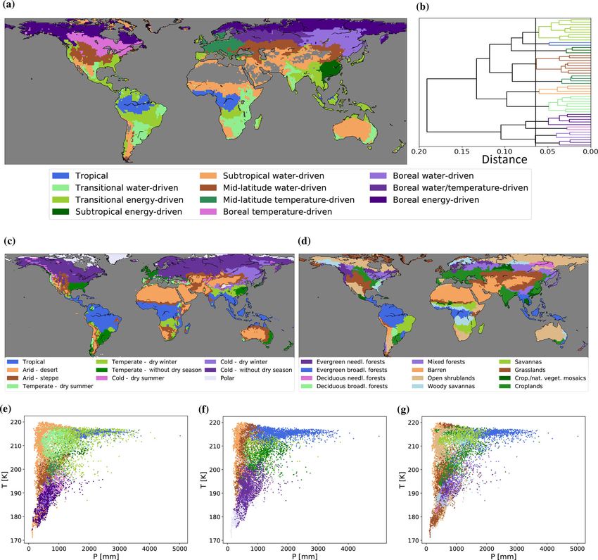
Figure 1. Graphical representation of two learning approaches. (a) A single-task learning approach in which each pixel is treated separately.
For each pixel l there is an input dataset X(l) ∈ RN×d , with N being the number of observations and d being the number of predictors, and a
target vector y (l) ∈ RN . The vector w (l) ∈ Rd represents the weight vector learned by the model. (b) A multitask learning approach in which
the models of L tasks are simultaneously learned. The input of the method is the datasets X(1) , X(2) , . . . , X(L)
h of all locations (i.e.iall global
land pixels). The corresponding target vectors are denoted with y (1) , y (2) , . . . , y (L) . The weight matrix w(1) , w (2) , . . . , w(L) ∈ Rd×L
contains the weight vectors for all tasks.
2014). It has also been used in climate science to improve tion of the notation in Fig. 1b. Given a loss function L (e.g.
the way multiple Earth system model (ESM) outputs are the squared error loss), the multitask minimization problem
combined by treating the locations as different tasks (Sub- is formulated as
bian and Banerjee, 2013; McQuade and Monteleoni, 2013).
L X
N
In these studies, the idea is that in neighbouring locations
(l) (l)
X
min L w (l) x i , yi + w (1) , . . . , w (L) , (1)
(pixels which are close to each other), similar ESMs tend to w (1) , ... ,w(L) l=1 i=1
have similar performance. A recent study proposed a hierar-
chy of tasks, in which at a first level, tasks of each location where w(1) , . . . , w (L) is a factor which controls the relat-
are trained into an MTL setting, while at a second level, tasks edness among the tasks. In our setting, we assume that there
of each variable are sharing information (Gonçalves et al., is no prior knowledge about the relationship of the tasks (lo-
2017). In addition, for modelling spatio-temporal data, Xu cations) and we aim to apply a method that can discover these
et al. (2016) introduced an MTL framework in which local relationships.
models share a common representation based on the spatial In the literature, there are many MTL methods that are
autocorrelation. Although this kind of modelling is becoming trying to do two things simultaneously: learn a weight ma-
more common in climate science (e.g. Subbian and Baner- trix w (1) , w(2) , . . . , w (L) and another matrix which cap-
jee, 2013; McQuade and Monteleoni, 2013; Gonçalves et al., tures the task relationships simultaneously (Ando and Zhang,
2017; Xu et al., 2016), it has not been combined (to the best 2005; Chen et al., 2009; Zhou et al., 2011). In real appli-
of our knowledge) with clustering approaches in the context cations, there are scenarios in which the tasks of an MTL
of mapping land cover or climate–vegetation dynamics. problem follow a specific structure; i.e. some tasks are more
In this work, we focus on MTL methods that can discover related, whereas some others are unrelated. In order to iden-
the relationship between different tasks (locations) and re- tify this group structure, researchers have developed various
cover strong predictive structures of the vegetation response methods which have been referred to as clustered multitask
to climate. These are then used to conform hydro-climatic learning (CMTL) methods (Zhou et al., 2011). For instance,
biomes, i.e. regions of coherent vegetation behaviour with Xue et al. (2007) proposed a method which uses a Dirich-
respect to climate variability (see Sect. 3.3). To this end, we let process-based statistical model to identify similarities be-
use the same notation as before by denoting X(l) ∈ RN×d as tween related tasks, while Jacob et al. (2009) introduced a
the input data matrix of the predictor variables, y (l) ∈ RN framework which identifies groups of tasks and performs the
as the target vector for each location l, and w(l) ∈ Rd in learning at once. In the same direction, Wang et al. (2009)
which
(1) each value corresponds to a weight. We define as used an inter-task regularization term to take into consider-
w , w(2) , . . . , w (L) ∈ Rd×L as the weight matrix of all lo-
ation tasks which have been grouped in the same cluster in
cations
(1) such that the w (l) vector is the lth column of the a semi-supervised setting. More recently, Barzilai and Cram-
w , w , . . . , w (L) matrix – see a graphical representa-
(2)
mer (2015) suggested a method which explicitly assigns each
Geosci. Model Dev., 11, 4139–4153, 2018 www.geosci-model-dev.net/11/4139/2018/C. Papagiannopoulou et al.: Global hydro-climatic biomes identified via multitask learning 4143
task to a specific cluster, building a single model for each task CMTL method (Zhou et al., 2011) under a specific condi-
by using linear classifiers which are combinations of some tion: that the parameter k, which symbolizes the number of
basis. An alternative approach has been proposed by Zhou clusters in the CMTL approach, is equal to the parameter h
et al. (2011) in which the structure of the task relatedness is of the ASO method. This condition determines the number
unknown and is learned during the training phase. Interest- of clusters that should be used in the clustering phase of our
ingly, when case-specific conditions are fulfilled, this method framework because the objective of ASO is optimized based
is equivalent to the method by Ando and Zhang (2005), on the value of the parameter h. We reconsider this equiva-
known as alternative structure optimization (ASO), which lence in Sect. 3.2 where we discuss the number of clusters
belongs to the category of MTL methods that assume the that should be identified based on our analysis.
existence of a shared low-dimensional representation among Formally, ASO can be formulated as the following opti-
the tasks. The name of the method indicates that an alternat- mization problem:
ing optimization procedure is involved during the learning L X N
process since the weight matrix and the matrix which cap- (l) (l) (l) (l) 2
X
min L(w x i , yi ) + λ ku k2 , (3)
(l)
tures the shared low-dimensional representation are learned {w (l) ,v (1) },22T =I l=1 i=1
simultaneously. Typically, in these procedures, the optimiza-
tion of each part is separately performed, while the other part with ku(l) k22 being the regularization term
u = w(l) − 2T v (l) that controls the task related-
(l)
remains fixed. In our work, we apply the ASO method due
(l) (l)
to its simplicity and the fact that it does not need a lot of it- ness among L tasks, (x i , yi ) being the input vector and
erations to capture the information about the task relatedness the corresponding target value of the ith observation in a
that is needed. This is crucial for our application, since the particular location l, and λ(l) being a predefined param-
large size of the global database we use (Papagiannopoulou eter – see Fig. 2 for the graphical representation of the
et al., 2017a) puts severe limitations on the choice of method. notation.
(1) (2)During (L) the learning process the weight matrix
Another aspect is that by learning this low-dimensional rep- w ,w , ...,w and the matrix 2, which captures
resentation we can have a visual inspection of the “most pre- the shared low-dimensional representation, are learned
dictive common structures” for each region. In the following simultaneously. The regularization term ku(l) k22 , based on
section we explain in detail the ASO method used in our set- the value of the parameter λ, penalizes the differences
ting. between the weights on the initial high-dimensional space
and the weights on the low-dimensional space parameterized
2.4 Learning predictive structures from multiple tasks by 2.
There are several ways of solving the optimization prob-
The ASO algorithm proposed by Ando and Zhang (2005) lem in Eq. (3) (Ando and Zhang, 2005). Our main purpose
learns common predictive structures from multiple related is to extract the shared feature space 2 in order to apply a
tasks that are assumed to share a low-dimensional feature clustering on the low-dimensional feature space. In this fea-
space. Specifically, by applying this method, one learns one ture space, locations with similar predictive structures will
model function for each individual task and the learned be grouped into the same broader region. For this reason,
weight vector is decomposed into two parts: (a) a high- we adopt an ASO algorithm based on singular value de-
dimensional space and (b) a shared low-dimensional space composition (SVD) as proposed by Ando and Zhang (2005),
based on a feature map learned during the process. This fea- which achieves good performance even on the first iteration
ture map is a matrix which serves as a link between a high- of the method. As mentioned before, this is crucial to our
dimensional space and a low-dimensional space. In our case, application given the large number of tasks and the high-
L
L predictor functions f (l) l=1 are simultaneously learned
dimensional datasets. The steps of the SVD-based ASO are
by exploiting the shared feature space that underlines all presented in Algorithm 1.
tasks. This low-dimensional feature space is expressed in The SVD-based ASO method can be interpreted as a di-
the simple linear form of a low-dimensional feature map 2 mensionality reduction technique applied to the model space
across the L tasks. Mathematically, the function f (l) can be (i.e. weights). It should be stressed here that this method must
written as not be confused with PCA, which is usually employed on the
(l) (l) (l)
f (l) (x) = w (l) x i = u(l) x i + v (l) 2x i , (2) data space (input space of predictors) (Metzger et al., 2012;
Ivits et al., 2014). The goal of the ASO method is to de-
with 2 ∈ Rh×d being a parameter matrix with orthonor- tect the principal components of the parameter matrix, while
mal row vectors; i.e. 22T = I, where h is the dimension- PCA identifies the principal components of the input data
ality of the shared feature space, and w(l) , u(l) , and v (l) X. The goal of the ASO method can be achieved by consid-
are the weight vectors for the full feature space, the high- ering the models of multiple tasks as samples of their own
dimensional one (initial dimension d), and the shared low- distribution. Therefore, these samples can only be formed by
dimensional one (based on the h parameter), respectively. using an MTL approach in which there is access to the mod-
As mentioned before, the ASO method is equivalent to the els from multiple learning tasks. Moreover, in our work, we
www.geosci-model-dev.net/11/4139/2018/ Geosci. Model Dev., 11, 4139–4153, 20184144 C. Papagiannopoulou et al.: Global hydro-climatic biomes identified via multitask learning
atic biomes identified via multi-task learning 5
ple tasks There are several ways of solving the optimization prob- 50
lem in Eq. (3) (?). Our main purpose is to extract the shared
on predic- feature space 2 in order to apply a clustering on the low-
e assumed dimensional feature space. In this feature space, locations
fically, by with similar predictive structures will be grouped into the
nction for same broader region. For this reason, we adopt the Singu- 55
tor is de- lar Value Decomposition (SVD)-based ASO algorithm, pro-
space, and posed 2.
Figure ?, whichrepresentation
byGraphical achieves good of performance evenThe
the ASO method. oninput
the of the method is the datasets X(1) , X(2) , . . . , X(L) of all locations. The
ature map first iteration of
corresponding the vectors
target method.areAsdenoted
mentioned
with before,
y , y this
(1) (2) , . .is
. , cru-
y (L) . The weight vector w(l) ∈ Rd of the full space is decomposed into two
a matrix cial to our application given
(l) the
d large number of tasks
parts: to the weight vector u ∈ R of the high-dimensional space and and the weight vector v (l) ∈ Rh of the low-dimensional one. The low-
dimensional feature map 2T ∈ Rd×h is common for all the tasks.
explicitly consider the climatic variables as predictors and
the vegetation variable as a target variable, and we learn the
relationship between them in a supervised setting. As such,
the regions that we define rely on the relationship between
climate and vegetation in a prediction setting, and the clus-
tering is calculated based on the similarity of this relation-
ship (i.e. the model coefficients for different locations); see
Sect. 2.5 for more details. As such, we learn relationships be-
tween climate and vegetation in a supervised setting, whereas
PCA-based methods (Metzger et al., 2012; Ivits et al., 2014)
are fully unsupervised. In our study the SVD decomposition
is used as part of the optimization algorithm and thus in a
supervised setting. In this setting, the model weights are op-
timized based on a given training set. Therefore, the discov-
ered structures are obtained during the training process.
To clarify the notation used in the ASO method, we intu-
itively explain the symbolization of the method in relation to
our specific setting: the problem of detecting locations with
similar climate–vegetation dynamics. As mentioned above
(Sects. 2.2 and 2.3), the input features that constitute the
X(l) ∈ RN×d matrix consist of the climatic predictor vari-
ables, i.e. the extreme indices and lagged variables, calcu-
lated based on raw climatic time series of a certain location
l. The dimensions N and d correspond to the number of ob-
(i.e., weights). It should be stressed here that this method
k22 (3) must not be confused with PCA, which is usually employed 65
Geosci. Model
on the data spaceDev., 11,space
(input 4139–4153, 2018 (??). The goal of
of predictors) www.geosci-model-dev.net/11/4139/2018/
the ASO method is to detect the principal components of the
= w (l) − parameter matrix, while PCA identifies the principal compo-
g L tasks, nents of the input data X. The goal of the ASO method canC. Papagiannopoulou et al.: Global hydro-climatic biomes identified via multitask learning 4145
T
servations, i.e. the length of the time series and the num- V = v (1) , . . . , v (L) ∈ RL×h matrix, which is the represen-
ber of predictor variables, respectively. The target variable tation of the models in this low-dimensional space, using the
for a particular location l, which is the NDVI anomalies, SVD-ASO method – see Sect. 2.4. The V matrix captures
is symbolized with y (l) ∈ RN . As such, an observation of a the information of the similar predictive structures among all
certainlocation l at a particular timestamp i is denoted as the tasks, so similar tasks are closer in this low-dimensional
(l) (l)
a pair x i , yi . The goal of the ASO method is to learn space and as a consequence they have a similar represen-
tation (i.e. weights) in this matrix. That way, the clustering
the weight matrix w (1) , w (2) , . . . , w(L) , i.e. a single weight
techniques based on distance calculations are applied on the
vector w(l) for each location l. This weight vector w(l) is more expressive low-dimensional space, resulting in a bet-
able to capture the relationship between the predictor vari- ter performance. As has been discussed in our previous work
ables and the target, i.e. the climatic variables and the NDVI (Papagiannopoulou et al., 2017a), global climate–vegetation
anomalies. Therefore, climatic predictors that are more im- relationships are complex and non-linear. Here, if the V rep-
portant for vegetation anomalies correspond to higher abso- resentation is expressive enough, the clustering method can
lute values in the weight vector w (l) . As a result, locations group together locations with similar models, i.e. locations in
with similar weights are considered as regions where vegeta- which vegetation responds to climate in a similar non-linear
tion responds to climate in a similar way. As described in a way. Thus, it is first necessary to evaluate the quality of the
previous paragraph of this section, the ASO method assumes learned matrix V. The most straightforward way to do so is
that the weight vectors w (l) consist of two parts: the u(l) and by measuring the predictive performance of the MTL model
the v (l) 2. These two parts are learned simultaneously in Al- in terms of e.g. R 2 . If the predictive power of the model is
gorithm 1 in an alternating fashion. The first part, i.e. the strong, we can conclude that the V matrix is able to capture
u(l) ∈ Rd , belongs to the high-dimensional space, the initial the relationships of each task well with the highly predictive
one, which is equal to d. This part expresses the location- structures. So, given that the V representation is sufficiently
specific part of the weight vector, i.e. the deviation of each learned from the data, we can apply any kind of clustering
location’s weight vector from the weights learned in a lower algorithm on the low-dimensional representation of matrix
dimensional space. The second part consists of the matrix V. This approach is also known as spectral clustering due to
2 ∈ Rh×d that represents the map from the initial dimension the fact that the clustering algorithm is applied on a reduced
d to the lower dimension h and the weight vector v (l) ∈ Rh . feature space, making the clustering results more robust.
The map matrix 2 is common for all the locations (tasks) In our application, we use a hierarchical agglomerative
and can be learned across them due to the MTL approach. clustering approach (Ward, 1963) in which the number of
The weight vector v (l) represents the projection of the initial clusters is not predefined. In the hierarchical clustering ap-
weights to a low-dimensional space h. Intuitively, this second proach, the result is usually depicted as a dendrogram in
part of the weight decomposition expresses the coarsest and which the leaves represent the observations and the in-
most important part of the weights, since it detects the most ner nodes correspond to the data clusters. The dendrogram
important structures through the map matrix 2. The matrix branches are proportionally long to the value of the inter-
T
V = v (1) , . . . , v (L) ∈ RL×h denotes the representation of
group dissimilarity. By defining this hierarchical form of the
the models in the low-dimensional space h for the L loca- clustering result, one can define the number of clusters by
tions. cutting down vertically (or horizontally, depending on the
view) the dendrogram in a point at which the dissimilarity
2.5 Land classification: clustering highly predictive between the clusters is high and therefore the branches are
structures longer – see Sect. 3.2 for the choice of the optimum number
of clusters in our analysis.
Clustering in machine learning is the task of grouping a set
of samples in such a way that those samples that belong 2.6 Experimental set-up
to the same group (cluster) are more similar with respect
to a specific criterion than to samples that belong to other In all the experiments, we use as predictors all the climatic
groups. Clustering techniques are usually based on a distance datasets and the features that we have constructed from them
(or similarity) measure, which is calculated among the sam- as well as the 12 lagged values of the target variable. A re-
ples and/or group of samples. There are several clustering sulting number of 3209 predictor (climate) variables is used;
approaches and an in-depth review can be found in Xu and i.e. d = 3209 in our setting. These variables constitute the in-
Tian (2015). put to our framework, i.e. the X(l) , l = 1, . . . , L datasets. As
It is known that in high-dimensional spaces, distance the target variable, we use the NDVI seasonal anomalies cal-
measures are not able to capture the differences between culated as in Papagiannopoulou et al. (2017a) and denoted
pairs of samples well, and thus clustering algorithms tend as y (l) , l = 1, . . . , L for each location. For more details about
to perform better in lower dimensional spaces. In our set- the datasets in our setting see Sect. 2.1. We examine 13 072
ting, we learn the common feature map 2 ∈ Rh×d and the land pixels with each pixel constituting a single task in our
www.geosci-model-dev.net/11/4139/2018/ Geosci. Model Dev., 11, 4139–4153, 20184146 C. Papagiannopoulou et al.: Global hydro-climatic biomes identified via multitask learning
MTL setting; i.e. L = 13 072. The dataset of each single task existence of a hidden structure between the different loca-
consists of 360 monthly observations given our 30-year study tions (tasks), which is informative with respect to our tar-
period; i.e. N = 360. get variable. The dotted regions in Fig. 3b correspond to ar-
For the STL modelling, evaluated for comparison, we use eas where the MTL model significantly outperforms the STL
the ridge regression for each location independently. Ridge models based on the Diebold–Mariano statistical test, which
regression is a linear model which uses an `2 norm regular- compares model predictions (Diebold, 2015). For the sta-
ization term in order to shrink the weight coefficients towards tistical test, we use the false discovery rate (Benjamini and
zero and avoid over-fitting. In ridge regression the weight Hochberg, 1995) method to correct the p values at level 0.05
coefficients are fitted by solving the following optimization due to the multiple-hypothesis testing setting.
problem: Additionally, Fig. 3a shows that more than 40 % of the
N
mean monthly vegetation dynamics can be explained by cli-
mate variability in some regions. In particular, in regions
L w(l) x i , yi + λ||w (l) ||2 ,
(l) (l)
X
min (4)
w(l) i=1 such as Australia, Africa, and Central and North America, the
predictive power of the model is stronger in terms of R 2 , fol-
with λ being a regularization parameter tuned using a sep- lowing the same pattern and scoring similar R 2 values as the
arate validation set and ||w (l) ||2 being a penalty term, i.e. random forest approach by Papagiannopoulou et al. (2017a).
the squared `2 norm of the weight vector. Note that by split- To elaborate on the performance difference between the two
ting the original dataset into three parts – (1) training set, approaches, the R 2 scores are presented as two different dis-
(2) validation set, and (3) test set – we tune the param- tributions in Fig. 3c. The blue histogram corresponds to the
eters in a set of observations (validation set) that are not distribution of the R 2 scores of the STL approach, while the
included in the final test set and achieve a fair evaluation orange one corresponds to the distribution of the R 2 scores
of the model performance. The optimization problems of of the MTL approach. As can be observed, the distribution
the SVD-ASO algorithm are solved by using the limited- of the R 2 scores is shifted to the right for the MTL, mean-
memory Broyden–Fletcher–Goldfarb–Shanno (L-BFGS) op- ing that values are typically greater than those derived from
timization algorithm. the STL approach. Moreover, the skew towards the left in the
blue histogram, with values close to zero, is an indication of
3 Results and discussion the near-zero performance of the STL models in many lo-
cations. The Wilcoxon paired statistical test (Demšar, 2006)
3.1 Single-task versus multitask learning model confirms that the results of the two approaches are overall
statistically different (p value < 10−9 ).
In a first experiment, we compare the predictive performance Since we are ultimately interested in investigating regions
of the STL model versus the MTL model. For the STL mod- of coherent impact of climate variability on vegetation dy-
elling, ridge regression is used. For the MTL modelling, we namics, we also evaluate the ability of the MTL model to de-
apply the ASO-MTL model (Ando and Zhang, 2005) de- tect Granger causal effects of climate on vegetation. For a de-
scribed in Sect. 2. We use a separate validation set to tune tailed description of the Granger causality modelling frame-
the regularization parameter λ for both approaches. For the work we direct the reader to Papagiannopoulou et al. (2017a).
STL approach, we tune the λ parameter for each location This point is crucial to understand the extent to which the
(task) separately, while for the MTL approach we use the climatic predictors carry additional information about the dy-
same λ value for all the tasks, taking into account the av- namics in vegetation that are not contained in the past vegeta-
erage performance across these tasks. For the ASO-MTL tion signal itself. The results of applying the Granger causal-
method, we have also experimented with the value of the ity analysis using MTL modelling are shown in Fig. 3d,
h parameter, which is the dimensionality of the shared fea- which illustrates the results of the full MTL model compared
ture space – see Sect. 3.2 for more details about the in- to the baseline MTL model. This baseline model only uses
fluence of this parameter on the clustering results. Finally, previous values of NDVI to predict monthly NDVI anomalies
we evaluate the performance of both approaches in terms (Papagiannopoulou et al., 2017a). In this figure it becomes
of R 2 , as in Papagiannopoulou et al. (2017a). Figure 3 de- clear that climate dynamics “Granger-cause” monthly vege-
picts the result of our comparison. Figure 3a shows the R 2 tation anomalies in most regions of the world, and the ability
of the ASO-MTL model, while Fig. 3b highlights the differ- of the MTL model to detect deterministic relationships is ev-
ence in predictive performance of the MTL model in com- idenced. This is also confirmed by the Wilcoxon paired sta-
parison with the STL model. As shown in Fig. 3b, in al- tistical test (p value < 10−9 ). On the other hand, the ability
most all regions of the world, the predictive performance of the STL model to detect Granger causal relationships is
increases substantially compared to the STL approach. In rather limited compared to that of the MTL model. Figure 3e
fact, over extensive regions (40 % of the study area), more depicts the result of the comparison; in almost all regions the
than 5 % of the variability in NDVI is explained by the spa- quantification of the Granger causality of the MTL approach
tial structure of the data. In statistical terms, this implies the increases substantially compared to the one of the STL ap-
Geosci. Model Dev., 11, 4139–4153, 2018 www.geosci-model-dev.net/11/4139/2018/C. Papagiannopoulou et al.: Global hydro-climatic biomes identified via multitask learning 4147
Explained variance (R2) of the MTL model Granger causality of the MTL model
.4 .2
.3
.1 .1
.05 .05
0 0
Difference (R2) between MTL and STL models Difference GC between MTL and STL models
.1 .1
.05 .05
0 0
-.05 -.05
-.1 -.1
750
R 2 STL GC-STL
R 2 MTL 750 GC-MTL
500
500
250
250
0 0
1.0 0.5 0.0 0.5 1.0 1.0 0.5 0.0 0.5 1.0
Figure 3. Comparison of the predictive performance between the STL and the MTL approaches. (a) Explained variance (R 2 ) of the NDVI
monthly anomalies based on the MTL approach. (b) Difference in terms of R 2 between the MTL and the STL approaches; blue regions
indicate a higher performance by the MTL. The dotted regions correspond to areas where the MTL model significantly outperforms the STL
models based on the Diebold–Mariano statistical test (Diebold, 2015). (c) Comparison of the distributions of the R 2 scores in the STL and
in the MTL setting; the blue histogram corresponds to the STL, and the orange one to the MTL approach. (d) Quantification of Granger
causality for the MTL approach, i.e. improvement in terms of R 2 by the full MTL model with respect to the R 2 of the baseline MTL model
that uses only past values of NDVI anomalies as predictors; positive values indicate Granger causality (Papagiannopoulou et al., 2017a).
(e) Difference in terms of Granger causality between the MTL and the STL approaches; blue regions indicate a higher performance by the
MTL. (f) Comparison of the distributions of Granger causality in the STL and in the MTL setting; the blue histogram corresponds to the
STL, and the orange one to the MTL approach.
proach. Analogous to Fig. 3c, Fig. 3f compares the distribu- that the results of the two approaches are overall statistically
tions of Granger causality (i.e. the difference in predictive different (p value < 10−9 ). In summary, these findings high-
performance in terms of R 2 between the full and the baseline light the potential of using the low-dimensional feature rep-
model) between the STL and MTL approach. Once again, resentation learned from the data to fulfill our final objective,
the blue histogram corresponds to the distribution of Granger which is the detection of vegetated areas holding a similar
causality retrieved using the STL approach, while the orange response to climate via a clustering approach.
corresponds to the results of the MTL approach. The shift
to the right of the orange histogram shows the larger abil- 3.2 Appropriate number of hydro-climatic biomes
ity of the MTL model to reveal Granger causality between
climate and vegetation. Similar to the previous comparison,
As described in Sect. 2.5, there are multiple approaches that
the Wilcoxon paired statistical test (Demšar, 2006) confirms
can be used to define the number of classes in a clustering
www.geosci-model-dev.net/11/4139/2018/ Geosci. Model Dev., 11, 4139–4153, 20184148 C. Papagiannopoulou et al.: Global hydro-climatic biomes identified via multitask learning
problem. In our framework, we define the number of clusters causality approach by Papagiannopoulou et al. (2017b), as
by using a data-driven approach. In our analysis, we choose well as the prior knowledge on climate and land use clas-
not to use information from any predefined number of veg- sification, we define the hydro-climatic biomes as follows:
etation and/or climate classes existing in the literature, since (1) tropical, (2) transitional water-driven, (3) transitional
the ultimate goal is to identify land classes fully indepen- energy-driven, (4) subtropical energy-driven, (5) subtropical
dently and only based on the observed relationship between water-driven, (6) mid-latitude water-driven, (7) mid-latitude
vegetation and climate. To this end, we rely on the definition temperature-driven, (8) boreal temperature-driven, (9) bo-
of the number of clusters on the predictive performance of real water-driven, (10) boreal water–temperature-driven, and
the MTL model. In Sect. 2.3, it is stated that the ASO-MTL (11) boreal energy-driven. This nomenclature is broadly
approach shares the objective function of the CMTL method. based on latitude and main climatic drivers.
This only holds if the number of clusters (which is a prede- Figure 4c shows the 10 main climate regions of the
fined parameter in the CMTL method) is equal to the value Köppen–Geiger climate classification, which is based on
of the parameter h in the ASO-MTL method, which is the precipitation and temperature and their seasonality. On the
dimensionality of the common feature space. In light of this other hand, the International Geosphere–Biosphere Program
equivalence relation, we experimented with a wide range of (IGBP) (Loveland and Belward, 1997) land cover classifi-
values for h in a validation set, aiming to select the value of cation, depicted in Fig. 4d, is mostly based on plant func-
h that maximizes the model performance in terms of R 2 . As tional types. Without the need to prescribe any land cover
such, we conclude that the best predictive performance oc- or climate classification and only relying on the spatial co-
curs at h = 11 and that the appropriate number of biomes in herence in the vegetation response to climate anomalies, our
the clustering phase equals 11 – see Sect. S2 for more details. hydro-climatic biomes in Fig. 4a clearly depict some of the
The results of this hierarchical clustering (with Euclidean main characteristic patterns from these traditional classifi-
distance) can be visualized in a dendrogram representation, cation schemes. For instance, the region of North Asia is
which provides an indication about the optimal number of quite coherent in terms of climate based on the 10 climate
clusters that emerge from the dataset. Figure 4b depicts the classes shown here (Fig. 4c), but quite diverse in terms of
dendrogram formed by our framework, with the vertical cut- vegetation type (Fig. 4d); the hydro-climatic biomes show a
ting line separating the data into 11 clusters. This representa- clear distinction in the transition from shrublands (energy-
tion allows for a visual inspection of whether the choice of 11 driven) to coniferous forests (energy- and water-driven). In
clusters is in line with the dissimilarities in the observations. North America, the more energy-limited ecosystems along
As one can observe, our choice is reasonable, since the clus- the coasts emerge from the water-driven regions inland, and
ters at this point are quite dissimilar, based on the Euclidean a latitudinal behaviour is also depicted, partly reflecting the
distance metric, compared to hypothesized cutting lines ei- transition from croplands and grasslands into temperate and
ther before or after this point. In other words, the branches of boreal forests. Patterns in the tropics clearly differentiate
the dendrogram are already quite long at 11 clusters, indicat- between rainforest and transitional savannas, and in South
ing high dissimilarities between the resulting classes. America the different drivers of vegetation dynamics in the
arc of deforestation lead to a class change that is depicted
3.3 Hydro-climatic biomes by neither the Köppen–Geiger climate classification nor the
IGBP land cover classes. Finally the patterns found for arid
The final objective of this study is to uncover the regions and warm semi-arid regions (here referred to as “subtropical
in which vegetation responds in a analogous way to climate water-driven”) and their transition towards wetter and more
anomalies, here referred to as “hydro-climatic biomes”. In vegetated ecosystems agree with the expectations based on
the previous section, we investigated the appropriate num- vegetation (Fig. 4d) and climate (Fig. 4c).
ber of such regions based on the information contained in The comparison to the Köppen–Geiger and IGBP maps
our database. Figure 4a illustrates the spatial distribution serves only as a general evaluation or proof of concept for
of the emerging global hydro-climatic biomes. The colours our hydro-climatic biomes map, since in the end such maps
depicted correspond to those of the clusters in the dendro- are based on a different rationale and thus there is no in-
gram of Fig. 4b. Further analysis of this dendrogram, in tent to “outperform” these classification schemes. However,
combination with the spatial distribution of the clusters in it can be observed in this comparison that the hydro-climatic
Fig. 4a, shows that our framework can clearly differenti- biomes map in Fig. 4a combines information on climate
ate the bioclimatic behaviour of northern latitude ecosys- and vegetation zones by illustrating regions where vegetation
tems from those in middle and southern latitudes. The be- similarly interacts with the multi-month dynamics in climatic
haviour of tropical ecoregions is unsurprisingly closer to the and environmental conditions. This conclusion is confirmed
behaviour of subtropical ones, while boreal regions sharing by the scatter plots in Fig. 4e–g. Figure 4e depicts our hydro-
exposure to low-temperature anomalies have a more coherent climatic biomes of Fig. 4a in a climate space of mean annual
response to one another, forming the second main branch of temperature against precipitation, while Fig. 4f shows the
the dendrogram. Bearing in mind the results of the Granger same but for the Köppen–Geiger climate classes of Fig. 4c. In
Geosci. Model Dev., 11, 4139–4153, 2018 www.geosci-model-dev.net/11/4139/2018/C. Papagiannopoulou et al.: Global hydro-climatic biomes identified via multitask learning 4149 Figure 4. Comparison of the different land surface classification schemes. (a) Hydro-climatic biomes derived from the proposed framework. The region colours correspond to the colours of the clusters that are depicted in the dendrogram. (b) Dendrogram scheme of the clustering derived from the hierarchical agglomerative clustering on the low-dimensional representation of our model observations. The length of the dendrogram branches is a function of the inter-cluster dissimilarities. The vertical cutting line marks the data split into 11 clusters. The denomination of the different classes is supported by the results from Papagiannopoulou et al. (2017b). (c) Simplified Köppen–Geiger climate classification scheme. (d) IGBP land use classification scheme. (e) Climate space (i.e. mean annual temperature versus precipitation) for our hydro-climatic biomes in Fig. 4a. (f) Same as (e) but for the Köppen–Geiger climate classes in Fig. 4c. (g) Same as (e) but for IGBP in Fig. 4d. Fig. 4f, the five climate classes are well separated, since their that the scatter plot of Fig. 4e clearly lies between the two definition is based on these two climatic variables. On the previous classifications in terms of clustering. Boreal biomes other hand, Fig. 4g depicts the same information but for the correspond to cold climate classes, and the subtropical and IGBP map of Fig. 4d. In this figure, savannas, tropics, and mid-latitude water-driven biomes correspond to arid regions, shrublands appear again well clustered. It can be observed while the transitional biomes correspond to the savannas and www.geosci-model-dev.net/11/4139/2018/ Geosci. Model Dev., 11, 4139–4153, 2018
4150                          C. Papagiannopoulou et al.: Global hydro-climatic biomes identified via multitask learning

croplands. The clustering of biomes is also consistent with       et al., 2016) of ecosystem resilience, and benchmarking the
the global distribution of key climatic drivers reported by Pa-   dynamic response of vegetation in Earth system models.
pagiannopoulou et al. (2017b) based on random forests and
a Granger causality framework, since these biomes are ul-
timately defined based on the response of vegetation to cli-      Code and data availability. We use the implementation of Python
matic and environmental conditions. These common dynam-           for the L-BFGS optimizer, the singular value decomposi-
ics are identified by latent structures in our MTL approach; a    tion method, and hierarchical clustering (Scikit-learn Python
discussion on these latent structures is included in Sect. S3.    library; Pedregosa et al., 2011). The code for the ASO-
                                                                  MTL method (https://doi.org/10.5281/zenodo.1241047) has been
Moreover, we should note that the approach of spectral clus-
                                                                  uploaded to our GitHub repository (https://github.com/lhwm/
tering applied here allows for a robust result, as small per-
                                                                  hydro-climatic-biomes, last access: 20 September 2018). Data used
turbations in the datasets do not affect the overall clustering   in this paper can be accessed using http://www.SAT-EX.ugent.be
result. This conclusion is confirmed by the fact that even in     (last access: 20 September 2018) as a gateway.
tropical regions, where the uncertainty in the observations is
typically larger and the skill of the predictions is lower (see
Fig. 3), the different clusters are separated in a clear man-     The Supplement related to this article is available
ner. A discussion about the comparison of the three land sur-     online at: https://doi.org/10.5194/gmd-11-4139-2018-
face classification schemes (the hydro-climatic biomes, the       supplement
Köppen–Geiger climate classification, and the IGBP land use
classification) is presented in Sect. S4. Results for microwave
vegetation optical depth (VOD) (Liu et al., 2011) anomalies       Author contributions. CP, WW, and DGM conceived the study. CP
as an alternative to NDVI anomalies are consistent as shown       conducted the analysis. CP, DGM, and MD led the writing. All co-
in Fig. S7 in the Supplement.                                     authors contributed to the design of the experiments, discussion and
                                                                  interpretation of the results, and editing of the paper.

4   Conclusion                                                    Acknowledgements. This work is funded by the Belgian Science
                                                                  Policy Office (BELSPO) in the framework of the STEREO III
In this paper we introduced a novel framework for identify-       programme, project SAT-EX (SR/00/306). Diego G. Miralles
                                                                  acknowledges support from the European Research Council (ERC)
ing regions with similar biosphere–climate interplay dynam-
                                                                  under grant agreement no. 715254 (DRY-2-DRY). The authors
ics. Our framework combines a multitask learning (MTL)            thank Stijn Decubber for fruitful discussions. The authors also
modelling approach and a spectral clustering technique, and       sincerely thank the individual developers of the wide range of
it is applied to a global database of global observational cli-   global datasets used in this study. Finally, the authors thank the
mate records compiled by Papagiannopoulou et al. (2017a).         reviewers for their constructive feedback.
Comparisons to a typical single-task learning approach, in
which each task (in each location) is analysed separately, in-    Edited by: David Topping
dicate that learning about climate–vegetation relationships in    Reviewed by: Stephanie Horion and one anonymous referee
neighbouring or even remote locations can help predict lo-
cal vegetation dynamics based on climate variability. More-
over, our approach is able to detect shared hidden predic-
                                                                  References
tive structures among the tasks that enhance the performance
of the models. These predictive structures form the basis to      Ando, R. K. and Zhang, T.: A framework for learning predic-
which the clustering algorithm is applied to detect regions         tive structures from multiple tasks and unlabeled data, J. Mach.
where vegetation responds to climate in a similar way. We           Learn. Res., 6, 1817–1853, 2005.
demonstrate that, without the need to prescribe any land          Baker, B., Diaz, H., Hargrove, W., and Hoffman, F.: Use
cover information, our method is able to identify coher-            of the Köppen–Trewartha climate classification to evalu-
ent climate–vegetation interaction zones that emerge directly       ate climatic refugia in statistically derived ecoregions for
from the spatio-temporal variability in the data. These zones       the People’s Republic of China, Climatic Change, 98, 113,
agree with traditional global classification maps, such as the      https://doi.org/10.1007/s10584-009-9622-2, 2009.
                                                                  Bartholomé, E. and Belward, A. S.: GLC2000: a new approach to
Köppen–Geiger climate classification or the IGBP land cover
                                                                    global land cover mapping from Earth observation data, Int. J.
classification. We refer to these regions as “hydro-climatic
                                                                    Remote Sens., 26, 1959–1977, 2005.
biomes”. These wide regions can be used for various appli-        Barzilai, A. and Crammer, K.: Convex multi-task learning by clus-
cations in geosciences, such as unravelling anomalous re-           tering, in: Artificial Intelligence and Statistics, San Diego, Cali-
lationships between climate and vegetation dynamics at lo-          fornia, USA, 9–12 May 2015, 65–73, 2015.
cal scales, defining extreme values of vegetation response to     Baxter, J.: A Bayesian/information theoretic model of learning to
climate, exploring tipping points and turning points (Horion        learn via multiple task sampling, Mach. Learn., 28, 7–39, 1997.

Geosci. Model Dev., 11, 4139–4153, 2018                                              www.geosci-model-dev.net/11/4139/2018/
You can also read