IMPACT OF RESOLUTION ON LARGE-EDDY SIMULATION OF MIDLATITUDE SUMMERTIME CONVECTION - MPG.PURE
←
→
Page content transcription
If your browser does not render page correctly, please read the page content below
Atmos. Chem. Phys., 20, 2891–2910, 2020
https://doi.org/10.5194/acp-20-2891-2020
© Author(s) 2020. This work is distributed under
the Creative Commons Attribution 4.0 License.

Impact of resolution on large-eddy simulation of midlatitude
summertime convection
Christopher Moseley1,2 , Ieda Pscheidt3 , Guido Cioni1 , and Rieke Heinze1
1 Max Planck Institute for Meteorology, Hamburg, Germany
2 Department  of Atmospheric Sciences, National Taiwan University, Taipei City, Taiwan
3 University of Bonn, Bonn, Germany

Correspondence: Christopher Moseley (christopher.moseley@mpimet.mpg.de)

Received: 11 July 2019 – Discussion started: 20 August 2019
Revised: 6 January 2020 – Accepted: 27 January 2020 – Published: 10 March 2020

Abstract. We analyze life cycles of summertime moist con-             1   Introduction
vection of a large-eddy simulation (LES) in a limited-area
setup over Germany. The goal is to assess the ability of the          An adequate representation of the diurnal cycles of con-
model to represent convective organization in space and time          vection in atmospheric models is important for numerical
in comparison to radar data and its sensitivity to daily mean         weather prediction and climate simulations, not only for the
surface air temperature. A continuous period of 36 d in May           tropics (Ruppert and Hohenegger, 2018) but also for mid-
and June 2016 is simulated with a grid spacing of 625 m.              latitude summertime convection (Pritchard and Somerville,
This period was dominated by convection over large parts of           2009). For this purpose, cloud-resolving models (CRMs)
the domain on most of the days. Using convective organiza-            without deep cumulus parametrization are increasingly ap-
tion indices, and a tracking algorithm for convective precip-         plied thanks to growing computational power. Meanwhile,
itation events, we find that an LES with 625 m grid spacing           the first global simulations with grid spacings between 7
tends to underestimate the degree of convective organization          and 2.5 km have been performed (Stevens et al., 2019). This
and shows a weaker sensitivity of heavy convective rainfall           range is usually termed convection permitting, as not all rel-
to temperature as suggested by the radar data. An analysis            evant processes within convective cells are sufficiently re-
of 3 d with in this period that are simulated with a finer grid       solved. In fact, in some of these models shallow convec-
spacing of 312 and 156 m showed that a grid spacing at the            tion is parametrized in order to correct deficiencies in the
100 m scale has the potential to improve the simulated diur-          simulation of smaller updrafts. Regional limited-area mod-
nal cycles of convection, the mean time evolution of single           els allow for even higher resolutions with grid spacings in
convective events, and the degree of convective organization.         the sub-kilometer range with large-eddy simulations (LESs)
                                                                      where the large eddies of the turbulence spectrum are mod-
                                                                      eled explicitly as opposed to a fully parametrized turbulence
                                                                      spectrum in the convection-permitting simulations. Recently,
Copyright statement. The author’s copyright for this publication is   selected diurnal cycles over Germany have been simulated in
transferred to the Max Planck Institute for Meteorology, Hamburg,     a realistic LES setup with the model ICON-LEM (Heinze
Germany.                                                              et al., 2017) within the German funded project HD(CP)2
                                                                      (“High Definition Clouds and Precipitation for advancing
                                                                      Climate Prediction”). Previous studies have discussed the
                                                                      question of which resolution is optimal for a good represen-
                                                                      tation of the processes involved in deep convective updrafts.
                                                                      A semi-idealized study of days with precipitating convection
                                                                      by Petch et al. (2002) with grid spacings between 2 km and
                                                                      125 m showed that the horizontal resolution should be at least

Published by Copernicus Publications on behalf of the European Geosciences Union.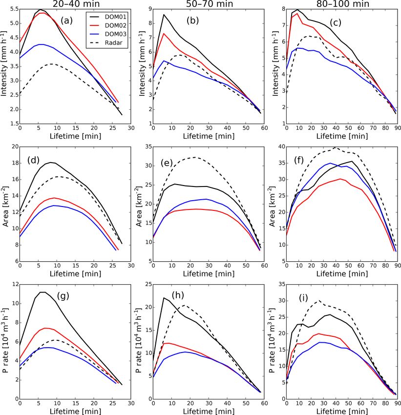
2892                                                         C. Moseley et al.: Impact of resolution on large-eddy simulation

one-quarter of the sub-cloud layer depth and that the best         tions. These parametrizations are particularly relevant at the
match with observational data was found only at the highest        abovementioned convection-permitting scale, and at present
resolution. Similarly, a study by Bryan et al. (2003) showed       we assume a random cloud distribution within model grid
that for an adequate simulation of a squall line using mod-        cells.
els with traditional LES closures, grid spacings of the order         Some studies that have investigated the sensitivity of con-
of 100 m are required. Besides horizontal resolution, there        vection to resolution distinguish between bulk convergence
are also other factors that impact the ability of CRMs to          and structural convergence (Langhans et al., 2012; Panosetti
simulate convection, such as the subgrid turbulence scheme         et al., 2019): while the former is concerned with large-scale
(Panosetti et al., 2019), the microphysics scheme (Singh and       mean properties, the latter refers to an analysis of cloud sizes,
O’Gorman, 2014), and the representation of the land surface.       cloud shapes, and convective organization. Our study mainly
   The formation of strong convective precipitation events         addresses structural convergence. To analyze the properties
depends on several environmental conditions, like air tem-         of convection and convective organization in model output
perature, surface fluxes, large-scale forcing, and the ability     and gridded observations like radar or satellite data, object-
of convection to organize. The sensitivity of precipitation ex-    oriented methods are increasingly applied. Besides simple
tremes to warmer temperatures has been heavily discussed in        mean values and percentiles of precipitation intensities, they
recent years. The argument that the strongest events should        provide information on the spatial distribution of sizes and
increase at a rate of ca. 7 % K−1 according to the thermody-       shapes of precipitation objects. Furthermore, several indices
namic Clausius–Clapeyron (CC) relation was put forward by          that are based on these methods have been developed over
Allen and Ingram (2002) and Trenberth et al. (2003). Obser-        recent years and are capable of quantifying the degree of or-
vational evidence showed that even in midlatitude regions,         ganization of the convection cells in space (Senf et al., 2018;
these rates can be up to twice the CC rate (Lenderink and          Pscheidt et al., 2019). Using a combination of several con-
Van Meijgaard, 2008; Westra et al., 2014), which is predom-        vective organization indices that we also apply in the present
inantly the case for convective precipitation, while the strati-   study, Pscheidt et al. (2019) have shown that convective pre-
form precipitation type follows CC more closely (Berg et al.,      cipitation cores and cloud tops are organized most of the time
2013). Meanwhile, several studies have found a super-CC            over Germany.
scaling for present-day climate. This indicates that beyond           However, the shortcoming of these methods is that they
purely thermodynamic processes, the dynamic component              provide only information on the spatial distribution of con-
within convective clouds also contributes to the intensifica-      vection objects, but not on their temporal evolution. Track-
tion and has to be evaluated separately. However, it has to        ing methods are able to additionally capture the life cycles
be mentioned that some studies have found a scaling that is        of the objects, and their interaction among each other. Sev-
close to the CC rate, like Ban et al. (2015), who argue that       eral tracking methods for convective storms have been devel-
the super-CC scaling might be an artifact that results from        oped in the past, and although they are based on similar ideas
the statistical methods applied to determine the scaling rate,     they are specialized for different purposes, such as nowcast-
e.g., the imposition of thresholds for wet days in the data        ing thunderstorms (Dixon and Wiener, 1993; Hering et al.,
analysis.                                                          2005; Kober and Tafferner, 2009; Wapler, 2017) and study-
   Analyses of climate change projections have indicated that      ing the cloud life cycle statistics in shallow (Heus and Seifert,
while the thermodynamic contribution to the intensification        2013; Heiblum et al., 2016) and deep convection (Lochbih-
of extreme precipitation is expected to be relatively homo-        ler et al., 2017; Moseley et al., 2019), or even larger struc-
geneous globally, there may be strong regional differences         tures like mesoscale convective systems (Fiolleau and Roca,
in the dynamic contribution due to changes in circulation          2013).
patterns (Emori and Brown, 2005; Pfahl et al., 2017; Norris           In this study, we apply the tracking method of Moseley
et al., 2019). CRMs should therefore also be able to simu-         et al. (2019), which provides statistical information on the
late the time evolution of convective precipitation events and     interaction of convective precipitation objects among each
their interaction and organization among each other in a re-       other in terms of merging and splitting. We analyze convec-
alistic way, to correctly represent their sensitivity to 2 m air   tive diurnal cycles simulated by the ICON-LEM with grid
temperature. Ban et al. (2014) have analyzed the temperature       spacings in the sub-kilometer range, and we assess the im-
scaling of a decade-long simulation with 2.2 km grid spac-         pact of horizontal resolution, and daily mean temperatures,
ing over Switzerland, and they found a good agreement with         on the simulated convection. This article is organized as fol-
observations. Kendon et al. (2014) have found an intensifi-        lows: in Sect. 2 we describe the ICON-LEM setup, the radar
cation of hourly rainfall over Britain under a climate change      dataset that is used for evaluation, and the object-oriented
scenario with a 1.5 km model. However, a correct represen-         analysis methods. In Sect. 3, we compare the simulation re-
tation of the temperature scaling of heavy rainfall becomes        sults of three different model resolutions between 625 and
increasingly difficult with decreasing model resolution. Rasp      156 m grid spacing, and in Sect. 4 we analyze a continuous
et al. (2018) have shown that in principle subgrid cloud orga-     36 d long simulation period with 625 m grid spacing. We dis-
nization has to be included in stochastic cloud parametriza-       cuss results in Sect. 5, and we present conclusions in Sect. 6.

Atmos. Chem. Phys., 20, 2891–2910, 2020                                             www.atmos-chem-phys.net/20/2891/2020/
C. Moseley et al.: Impact of resolution on large-eddy simulation                                                            2893

2     Data and methods                                             heavy convective precipitation, 10 tornadoes, and hail, which
                                                                   caused damages running into the billions of euros (Piper
2.1    Model configuration                                         et al., 2016). The strongest events were concentrated between
                                                                   26 and 29 May 2016 mostly over southern Germany, while
The simulations are performed with the unified modeling            during the first days of June a -blocking pattern over Eu-
framework ICON, which was run with the LES physics pack-           rope prevented the typical westerly flow from reaching cen-
age, in the following termed ICON-LEM (“ICON Large                 tral Europe and enhanced local instability caused by diurnal
Eddy Model”) (Dipankar et al., 2015). ICON is a non-               surface heating and nocturnal cooling.
hydrostatic new-generation model tailored to perform atmo-            To reduce computational costs, the entire 36 d period is
spheric simulations in different setups ranging from global        simulated only on the outermost nest (domain 1) with 625 m
climate reconstructions to limited-area nested configura-          grid spacing. The simulation is initialized on 26 May 2016
tions and idealized configurations. Different physics pack-        at 00:00 UTC and continuously run through 31 June 2016,
ages needed to parametrize sub-scale variability are adopted       00:00 UTC using only the forcing from the boundary condi-
depending on the setup considered. ICON has been used at           tions provided by hourly analysis of the COSMO-DE data
the German Weather Service (DWD) since 2015 to produce             at the lateral boundaries of the outer domain. Local features,
operational forecasts and has been successfully adopted as         such as individual clouds or thunderstorms, are mostly the
a tool to improve our understanding of moist convection in         results of local forcing and thus may look different from
many areas of the world (e.g., Klocke et al., 2017).               the observed ones, which is partially due to the inherent un-
   In our work, ICON-LEM is used in a limited-area config-         predictability of convection. A total of 3 d among this pe-
uration to perform convection-explicit simulations over Ger-       riod are simulated with the additional nests with 312 and
many. The model configuration follows the description given        156 m grid spacing (a more detailed description of the large-
in Heinze et al. (2017) very closely, to which the reader is re-   scale situation in this period over Germany is given by Rasp
ferred for further details on the parametrizations employed.       et al. (2018), who analyzed the period between 26 May and
We only emphasize that turbulence is parametrized using a          9 June 2016 in their study).
Smagorinsky model (Dipankar et al., 2015) (thus, subgrid
                                                                     – 29 May 2016 was dominated mainly by wind from the
turbulence is treated as isotropic), the land surface is de-
                                                                       southeast, with relatively widespread high level clouds
scribed using the TERRA-ML model (Schrodin and Heise,
                                                                       that grew larger throughout the afternoon and strong
2002), the surface layer is treated with a drag-law formula-
                                                                       convection over the largest part of the domain. At night,
tion following Louis (1979), a simple all-or-nothing cloud
                                                                       a mesoscale convective system developed that covered
scheme is used, and cumulus convection as well as gravity
                                                                       most of southern Germany.
waves (orographic and non-orographic) are not parametrized.
   At the boundaries, ICON is forced by operational hourly           – 3 June 2016 was characterized by moderate easterly
analysis data by the previous operational numerical weather            wind in the northern half of the domain with mainly
prediction (NWP) model COSMO-DE by the DWD, run with                   clear sky in the morning and broken convective cloudi-
ca. 2.8 km grid spacing. The model output is interpolated to           ness in the afternoon. The southern part of the domain
the ICON model grid with 625 m grid spacing, on which the              was dominated by strong convective rainfall, beginning
model simulations are performed. Dynamical downscaling                 around noon.
in a one-way nesting approach is applied on 3 of the model
days, in a first step to 312 m and in a second step to 156 m         – 6 June 2016 was characterized by weak easterly winds
grid spacing (Heinze et al., 2017). In this case, boundary con-        and a distinct diurnal cycle of convection with mainly
ditions for each one of the two inner domains are taken from           clear sky in the morning and convective cloudiness with
the relative outer domain (see Fig. 1).                                a maximum in the afternoon over the largest part of the
   We note that we restrict the evaluation of the ICON-LEM             domain, associated with increasing high-level cloudi-
simulations to daytime between 06:00 and 21:00 UTC, since              ness caused by stratiform outflow.
it is known that the nocturnal boundary layer is not suffi-           In all simulations, the state of the atmosphere and the soil
ciently resolved at LES resolutions of 100 m and coarser,          has been initialized at 00:00 UTC with COSMO-DE data.
which may introduce unknown biases in cloud cover at               The first 6 simulation hours are used as spin-up for the at-
night (van Stratum and Stevens, 2015). Therefore, the figures      mosphere and are removed from the analysis. For the high-
showing our results are also restricted to this period.            resolution three-domain simulations, all three nests are initi-
                                                                   ated at the same time.
2.2    Simulation period
                                                                   2.3   Preparation of model and radar data
We chose a period of 36 continuous days, beginning on
26 May and ending on 20 June 2016. This period includes            We use the RADOLAN RY C-Band weather radar compos-
an exceptional sequence of severe weather events producing         ite provided by the German Weather Service (Bartels et al.,

www.atmos-chem-phys.net/20/2891/2020/                                               Atmos. Chem. Phys., 20, 2891–2910, 2020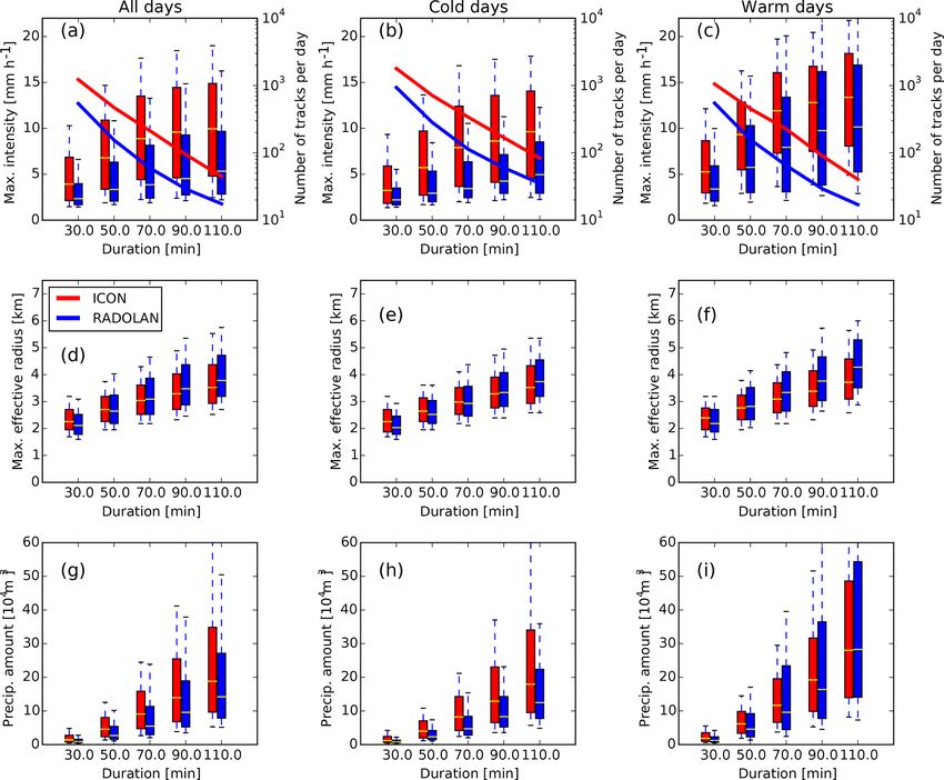
2894                                                           C. Moseley et al.: Impact of resolution on large-eddy simulation

                                                                     156 m grid spacing as shown in Fig. 1. Elsewhere, where we
                                                                     analyze only the outer domain with 625 m grid spacing, we
                                                                     include the full domain size.
                                                                        The temporal output interval of the model data is 2 min,
                                                                     while the radar data are available with a 5 min interval.
                                                                     Therefore, the modeled precipitation intensities have been
                                                                     linearly time-interpolated to a 5 min interval.

                                                                     2.4   Indices of convective organization

                                                                     To investigate whether convective clouds tend to organize in
                                                                     space, we follow the approach used in Pscheidt et al. (2019):
                                                                     first, we detect signatures of convection in radar and model
                                                                     rain rates by applying a segmentation algorithm with a split-
                                                                     and-merge approach (Senf et al., 2018) with a threshold of
                                                                     1 mm h−1 . In a second step, we compute commonly used or-
                                                                     ganization indices for the radar observations and the simula-
                                                                     tion output. The organization indices are based on the char-
                                                                     acteristics of the 2-D objects obtained from the segmentation
Figure 1. Simulation domain. The black frame shows the extent of
                                                                     algorithm. We employ three organization indices, namely the
the outer domain 1 with 625 m grid spacing, and the red and blue     Simple Convective Aggregation Index (SCAI; Tobin et al.,
frames show the nested domains 2 and 3 with 312 and 156 m grid       2012) and the convective organization potential (COP; White
spacing, respectively. The black contour shows the maximum extent    et al., 2018), which are both based on all-neighbor distances,
of the RADOLAN dataset. Color shading shows the surface precip-      and the Iorg index (Tompkins and Semie, 2017), which uses
itation field on 3 June 2016, at 14:00 UTC, simulated on the outer   a nearest-neighbor (NN) distance approach. SCAI is defined
domain with 625 m grid spacing, given in millimeters per hour.       as
                                                                              N D0
                                                                     SCAI =          1000,                                       (1)
                                                                              Nmax L
2004). This data product contains precipitation intensities
derived from radar reflectivities on a grid of approximately         where N is the number of objects in the domain, D0 is the
1 km × 1 km. We apply a conservative remapping to inter-             geometric mean distance of the centroids between all possi-
polate all model and radar data to a common lat–long grid.           ble pairs of objects, Nmax is the possible maximum number
This implies that we also evaluate the model data on the three       of objects that can exist in the domain, and L is the charac-
nests with 625, 312, and 156 m model grid spacing on the             teristic domain size. In this study, Nmax is the total number of
same target grid after interpolation. The main reason for in-        grid boxes in the domain, and L is the southwest–northeast
terpolating the model data is that the original ICON-LEM             distance in the domain. The degree of organization increases
output is given on an unstructured triangular grid which is          as the SCAI decreases.
difficult to handle for our post-processing tools. The second           COP considers√the interaction
                                                                                                 √        potential √
                                                                                                                    between two ob-
reason is that we prefer to compare the data of the three dif-       jects V (i, j ) = ( A(i) + A(j ))/(d(i, j ) π ), where A(i)
ferent model resolutions, and the radar data, on the same            is the area of object i and d(i, j ) is the Euclidean distance
grid, to reach a fair comparison. We chose a 1 × 1 km2 lat–          between the centroids of the objects i and j . COP is defined
long grid, since this is roughly the resolution of the radar         as
data. Further, it is only slightly coarser than the resolution                 PN PN
of the coarse ICON-LEM resolution with 600 m grid spac-                           i=1 j =i+1 V (i, j )
                                                                     COP =           1
                                                                                                       .                          (2)
ing of the triangle edges. However, as the effective resolu-
                                                                                     2 N (N − 1)
tion of the ICON-LEM data is larger than the grid spacing,
we can assume that there is no loss in resolution at least           The degree of organization increases as COP increases.
for the 600 m simulation. A similar regridding has also been            Unlike SCAI and COP, which mainly quantify the degree
used for other studies which also analyzed ICON-LEM out-             of clustering, the NN-based organization index Iorg (Tomp-
put (Heinze et al., 2017; Pscheidt et al., 2019).                    kins and Semie, 2017) is able to distinguish between three
   As the radar data contain areas of missing values that vary       types of spatial distribution: clustered, regular, and random.
in time when instruments were switched on and off, we also           In this approach, we treat objects as discs (similar to Nair
mask out these areas in the model data, to have a one-to-            et al., 1998), and we compute the cumulative distribution
one comparison. In Sect. 3, where we compare results of all          function of the NN edge-to-edge distances (NNCDF) and
three nests, we restrict the domain to the innermost nest with       compare it to the NNCDF of theoretical randomly distributed

Atmos. Chem. Phys., 20, 2891–2910, 2020                                               www.atmos-chem-phys.net/20/2891/2020/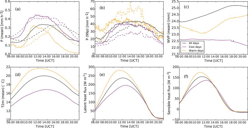
C. Moseley et al.: Impact of resolution on large-eddy simulation                                                               2895

objects over the same domain. The theoretical NNCDF is               the advection field while checking for overlaps. This step has
approximated by bootstrapping, in which a random num-                to be iterated until the object identification result converges.
ber of objects with the observed size distribution are ran-             In a third step, overlapping objects are combined to tracks.
domly placed over the domain (Weger et al., 1992; Nair et al.,       A fraction of the tracks have distinct life cycles and do
1998). We perform 100 simulations and compare the ob-                not merge with others or split up into fragments. They are
served NNCDF to the 100 theoretical NNCDFs in a graph.               initiated as new emerging precipitation events and eventu-
Iorg is defined as the area below such a comparison curve (for       ally vanish when surface precipitation ceases. We call these
more details see, e.g., Pscheidt et al., 2019; Tompkins and          tracks solitary. Tracks that experience merging and splitting
Semie, 2017). From the 100 computed Iorg indices we select           are recorded separately. We call these tracks interacting. A
percentiles 2.5 and 97.5 to identify the spatial distribution.       parameter, the so-called termination sensitivity 2 that takes
The objects are organized in clusters when percentile 2.5 is         values between 0 and 1, provides a criterion whether a merg-
greater than 0.5, whereas they present a regular distribution        ing or splitting event is recorded, or ignored. If 2 = 0, then
in space when percentile 97.5 is lower than 0.5. Otherwise,          every merging and splitting event will lead to a termination
the scenario can not be differentiated from randomness.              of all involved tracks and will be recorded as a track that in-
   In addition to the degree of convective organization, we          teracts with its neighbors. In the other extreme 2 = 1, the
also investigate the shape of the objects with the index Ishape      largest object that experiences a merging or splitting event
defined as                                                           will always be continued and regarded as solitary, while the
                                                                     smaller involved tracks will be terminated and not regarded
              N
           1 X                                                       as non-solitary. If 2 takes intermediate values, all participat-
Ishape =         s(i),                                        (3)
           N i=1                                                     ing tracks will only terminate when they are of comparable
                                                                     size, otherwise the largest one will be regarded as solitary and
where s(i) = Peq (i)/P (i) is the                                    the smaller one as interacting. For our analysis, we choose an
                               √ shape ratio, P (i) is the ac-
tual perimeter, and Peq (i) = 4π A(i) is the perimeter of            intermediate value of 2 = 0.5.
an equivalent, area-equal disc of the object i. The perime-
ter P (i) is computed as the contour line through the centers
of the border grid boxes of the objects (Benkrid and Crookes,        3     Impact of resolution
2017; van der Walt et al., 2014). Ishape ranges between 0 and
1 and indicates the predominant presence of linear shapes for        3.1    Domain mean precipitation and size distribution
the former and circular shapes for the latter. Ishape close to 0.5
indicates predominance of elliptical shapes.                         To analyze the impact of resolution on the simulated life
                                                                     cycles of convection, we make use of the 3 d which have
2.5   Rain cell tracking                                             been simulated on three nests with 625 m (DOM01), 312 m
                                                                     (DOM02), and 156 m (DOM03) grid spacing. Figure 2 shows
We apply the “iterative rain cell tracking” (IRT) algorithm to       the time series of the daily mean precipitation for each day
track life cycles of convective precipitation events in space        for all three domains next to the radar data, averaged over all
and time (Moseley et al., 2019). In a first step, precipitation      areas where radar data are available. While on 29 May the
objects are detected for each time step individually. They are       simulated precipitation amount for all three domains is very
defined as connected areas over a given threshold chosen as          close and strongly mismatches the radar data, on the other
1 mm h−1 surface precipitation intensity. This threshold has         2 d on 3 and 6 June the time evolution of mean precipita-
proven to generate reasonable results, and is on the order of        tion differs more strongly for the different resolutions. On
the resolution threshold of the weather radar. For each ob-          the last 2 d, the match with RADOLAN is better for higher
ject, the area and the mean surface precipitation intensity          resolutions: the peak precipitation on the 625 m domain is
averaged over this area are recorded. The algorithm checks           larger and is reached earlier than for the 312 and 156 m nests.
for overlaps of each object with objects in the previous and         Especially on 3 June, both the magnitude and the timing of
the subsequent time step, and records the concerning object          the precipitation peak are closer to the radar data for the do-
identifiers. If an object overlaps with more than one object at      mains with higher resolutions than for the 625 m domain. On
the previous or subsequent time step, the two largest ones are       both 3 and 6 June, the strong increase in precipitation around
recorded; others are ignored.                                        10:00 UTC is steeper than in the radar data for 625 m, while
   It sometimes happens that objects of subsequent time steps        the slope matches the radar data best for 156 m. However,
do not overlap although they belong to the same track, since         on 6 June the decline of precipitation intensity in the late
they are advected by mean background flow, especially if the         afternoon and evening hours appears too late. We note that
time step is relatively large and the objects are small. To cor-     although the later onset in the simulations with higher res-
rect this artifact, in a second step a mean background ad-           olution appears to be consistent on 3 and 6 June, we can-
vection field is diagnosed and the procedure is repeated by          not rule out that some of the other differences may be due
taking into account the displacements of the objects due to          to internal variability, like individual large storms. Simulated

www.atmos-chem-phys.net/20/2891/2020/                                                 Atmos. Chem. Phys., 20, 2891–2910, 2020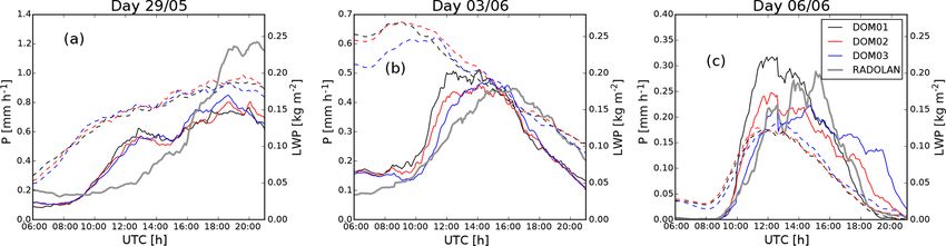
2896 C. Moseley et al.: Impact of resolution on large-eddy simulation
cloud water follows the total precipitation intensity closely for the 156 m nest for the days 29 May and 3 June, with de-
on the days 29 May and 6 June, while the high values of liq- creasing performance for the coarser nests (Fig. 4j, k).
uid water path (LWP) in the morning hours on 3 June indicate For 6 June, the diurnal cycle of the COP and Iorg shows
non-precipitating cloudiness, which was found mainly in the a different behavior than on the other 2 d: COP is in good
southern part of the domain. agreement with radar between 09:00 and 17:00 UTC for all
Rain cell size distributions for all three nests and three grid spacings (Fig. 4f). In the evening, however, the
RADOLAN are shown in Fig. 3, including the rain cell ob- simulations with the finest nests reveal larger object sizes
jects of all three-domain days. Compared to the 625 m nest, (not shown) than observed in radar, leading to an overesti-
the RADOLAN data show a larger fraction of large objects, mation of the degree of clustering. Besides, no objects are
but fewer small objects that can be attributed to isolated cells. detected in the 625 m nest after 19:00 UTC. The increased
However, the total number of large clouds in the radar data is oscillation in the degree of clustering after 20:00 UTC seen
not much different from the simulations. For the more highly in COP is reflected in Iorg and indicates spatial distributions
resolved nests, the fraction of small objects is closer to radar. varying between clustering and random distribution (Fig. 4i).
This picture is consistent if the size distribution is plotted for Regarding the object’s shapes, the coarsest nest shows the
each of the days individually (not shown). best performance for this day, though (Fig. 4l).
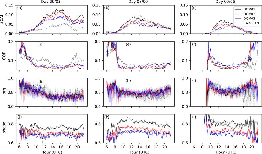
An interesting observation is that SCAI differs more
strongly between the days, while for the other indices, the
3.2 Convective organization indices
differences among the simulation nests and the radar data
are of the same order as the differences between different
A general convergence of the higher-resolution nests to the days. The reason could be that SCAI closely follows the to-
RADOLAN data is found not only in the diurnal cycles of tal number of rain cells, which varies strongly between days,
mean precipitation and the cell size distribution, but also in while the other indices are rather linked to the size distribu-
the organization indices that we have calculated for the three tion, which is similar on all 3 d.
domains and the RADOLAN data, especially in SCAI and
Ishape (Fig. 4). In general, SCAI tends to follow the mean 3.3 Track statistics
precipitation intensity, rather than the mean amount of cloud
water (Fig. 2). The analysis of SCAI reveals that on 29 May We apply the tracking algorithm to the precipitation cells of
the radar objects are more clustered than the simulated ones model and RADOLAN data (note that all data are evaluated
(Fig. 4a); however, the finest nest is closest to RADOLAN. on the domain of the innermost nest and on the same grid),
The 156 m nest also shows the best performance on 6 June, and we build a single sample containing all tracks of the 3 d.
when the degree of organization of observed objects is very In total, the algorithm detects 141 682 tracks for DOM01,
well represented at 156 m (Fig. 4c). The situation is, how- 160 042 tracks for DOM02, and 124 820 for DOM03, show-
ever, different for 3 June (Fig. 4b). Before 12:00 UTC the ing no clear trend with resolution. For the radar data, a
finer nests best represent the degree of organization, whereas smaller number of 67 657 tracks is detected. We perform a
from 12:00 until 18:00 UTC, the coarsest nest is in better separate analysis for solitary tracks (i.e., tracks that do not
agreement with radar. On all 3 d, SCAI shows a clear increase merge or split), tracks that involve only merging (i.e., tracks
in the degree of clustering with the nest’s resolution, which that either merge into others or are initiated by merging of
is due to the decrease in the number of small objects as the other tracks, but that do not involve splitting), tracks that in-
grid spacing increases (see the size distribution in Fig. 3). volve only splitting (i.e., tracks that split up, or tracks that are
Although the size distribution does not provide any direct in- initiated as a fragment of a splitting event), and tracks that
formation on the shape of objects, the smaller value of Ishape involve both merging and splitting (i.e., tracks that either are
in the radar data is consistent with the larger fraction of large initiated as a merging event and split up later or are initiated
objects, since large objects are more likely to deviate strongly as a fragment and later merge again with other tracks); see
from the circular shape (Fig. 4j–l). Table 1. Although less than 10 % of the total rainfall is gen-
The COP index indicates more clustering of the radar ob- erated by solitary tracks (excluding drizzle below the thresh-
jects than in the simulations in the course of the days, es- old of 1 mm h−1 and tracks that touch the boundaries), there
pecially on 29 May and 3 June, due to the smaller sizes of is a strong variation in the contribution of solitary tracks to
the simulated objects (Fig. 4d, e; note also the size distribu- the total rainfall, namely 9.4 %, 7.1 %, and 4.2 %, indicating
tions in Fig. 3). A clustered distribution is also reinforced by the tendency toward more organization with increasing res-
Iorg (Fig. 4g–i), indicating convective organization through- olution. For comparison, for RADOLAN we find a fraction
out the day with a slight decrease in the degree of cluster- of 6.7 %, which is between the model results of the 312 and
ing in the afternoon in agreement with SCAI and COP. The 156 m nest. The ratio of the number of tracks belonging to all
simulations represent Iorg in all three grid spacings well, and track types is very similar for all nests and matches well with
significant differences among the three grid spacings are not RADOLAN, but there are differences in the contribution to
found. In contrast, the shape of the objects is best represented total rainfall among these types. There is a clear increase with
Atmos. Chem. Phys., 20, 2891–2910, 2020 www.atmos-chem-phys.net/20/2891/2020/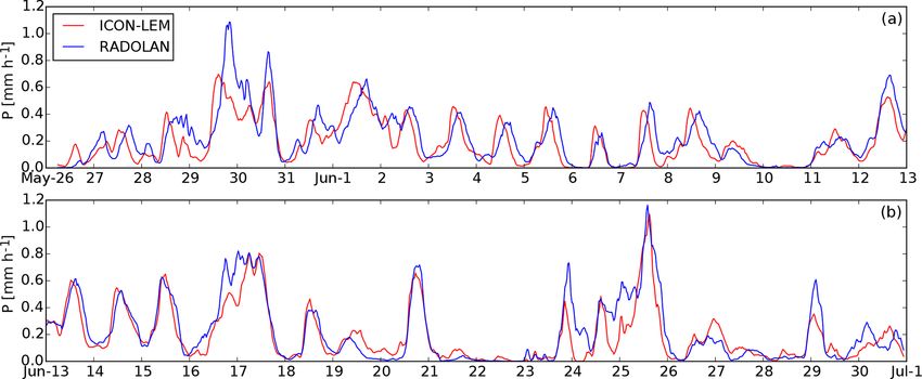
C. Moseley et al.: Impact of resolution on large-eddy simulation                                                                    2897

Figure 2. Time series of the mean precipitation intensity P (solid lines, left axes) and liquid water path LWP (dashed lines, right axes),
for the 3 d 29 May (a), 3 June (b), and 6 June (c), for all three domains with 625 m (DOM01), 312 m (DOM02), and 156 m (DOM03) grid
spacing. The gray thick line shows the RADOLAN derived precipitation intensity. Averaging was carried out over all grid boxes where radar
data are available.

                                                                       provement with increasing resolution compared to the radar
                                                                       data: sizes are smaller in the model data than in RADOLAN,
                                                                       except for short-duration tracks in the 625 m domain. In con-
                                                                       trast to intensity, track maximum extents of the 625 m do-
                                                                       main show a better match with RADOLAN, while the sizes
                                                                       of tracks of the 312 m and 156 m nests are clearly smaller
                                                                       (Fig. 5d–f). The rate of total precipitation produced by the
                                                                       solitary rainfall events (i.e., the spatial integral of precip-
                                                                       itation intensity integrated over the object area shown in
                                                                       Fig. 5g–i), however, shows that for intermediate- and long-
Figure 3. (a) Normalized probability density function (PDF) of rain    duration tracks simulated with 625 m grid spacing, the too
cell size distributions, on all three domains DOM01, DOM02, and        large intensities are compensated for by the too small intensi-
DOM03 and the RADOLAN data. (b) Same as (a), but with total            ties, resulting in a good match with RADOLAN, while rates
number of cells on the vertical axis (in bins of width 10 km2 ). The   are clearly too small for the finer nests. Only for the short-
PDF includes all rain cells between 06:00 and 21:00 UTC on all 3 d     duration tracks, does the precipitation rate of the 156 m nest
(29 May, 3 June, 6 June).
                                                                       agree with RADOLAN, while the coarse resolution produces
                                                                       too much precipitation.
                                                                          We further visualize the statistics of the solitary track peak
resolution from 29.5 % (for DOM01) to 47.2 % (DOM03) for
                                                                       intensities, the maximal effective radii √ of the objects (where
the type that experiences both merging and splitting. As this
                                                                       the effective radius is given as ri = Ai /π, with Ai being
track type can be regarded as the one that experiences the
                                                                       the area of object i), and the total precipitation amount pro-
strongest interaction with neighboring tracks, the high rain-
                                                                       duced by the tracks (given as the spatial integral over the
fall ratio falling onto this track type in the 156 m nest indi-
                                                                       area and the temporal integral along the track duration of the
cates a stronger impact of convective organization. However,
                                                                       local intensity) in the box-and-whisker plots in Fig. 6. The
for RADOLAN, this ratio is only 32.4 %, which is close to
                                                                       solid curves in Fig. 6a show that in total there are more soli-
the coarse-resolution result.
                                                                       tary tracks found in the model data than in RADOLAN, but
   Even though solitary tracks contribute to less than 10 %
                                                                       for longer durations, curves for RADOLAN and the 156 m
of the total precipitation, they are most suited for an analy-
                                                                       nest converge. The decreased number of longer-lasting soli-
sis of the time evolution of convective rainfall events. There-
                                                                       tary tracks reflects the stronger organization in the high-
fore, we have a closer look at the performance of the model
                                                                       resolution domain, since stronger convective events are more
to simulate solitary track life cycles. Mean life cycle com-
                                                                       likely to interact with neighboring tracks. As already indi-
posites of the 3 three-domain days, comparing model and
                                                                       cated by the life cycles in Fig. 5, we see that the median of
RADOLAN tracks and conditioned on short (20–40 min), in-
                                                                       peak intensities is lowest for the finest resolution and shows
termediate (50–70 min), and long (80–100 min) track dura-
                                                                       a good match with RADOLAN, while peak intensities reach
tions, are shown in Fig. 5. The curves show that generally the
                                                                       higher values for the 625 m domain. However, the spread in
mean peak intensities decrease for higher resolutions, while
                                                                       peak intensities is much higher for the RADOLAN data for
the largest jump is visible between 312 and 156 m grid spac-
                                                                       longer-duration tracks, while it is lowest for the 156 m nest, a
ing (Fig. 5a–c). The match with RADOLAN intensities is
                                                                       feature that is not visible in the mean life cycles in Fig. 5. Fur-
best for the 156 m nest. The track sizes do not show an im-

www.atmos-chem-phys.net/20/2891/2020/                                                    Atmos. Chem. Phys., 20, 2891–2910, 2020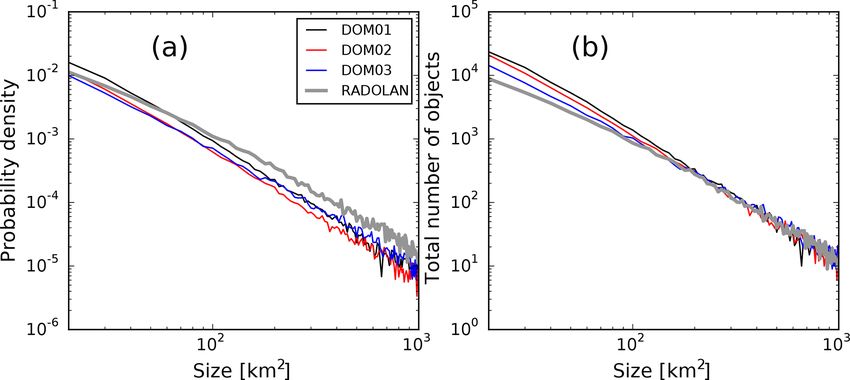
2898                                                              C. Moseley et al.: Impact of resolution on large-eddy simulation

Figure 4. Convective organization indices SCAI (a–c), COP (d–f), median Iorg (g–i), and Ishape (j–l) for the days 29 May and 3 and
6 June 2016, for the three nests with 625 m (DOM01), 312 m (DOM02), and 156 m (DOM03) grid spacing and the RADOLAN data.
Averaging was carried out over all grid boxes within the 156 m nest where radar data are available.

Table 1. Ratio of the number of tracks of given track types (solitary, tracks that involve only merging, tracks that involve only splitting, and
tracks involving both merging and splitting) and the total amount of rainfall that they contribute, relative to the total number and rainfall
amount, respectively, of all tracks. Note that tracks that touch the domain boundaries are removed from the analysis. Fractions (in percent),
including all 3 three-domain days, are given for all three domains with 625 m (DOM01), 312 m (DOM02), and 156 m (DOM03) grid spacing
and for the RADOLAN composite.

                            Ratio (number; amount) (%)         DOM01         DOM02        DOM03       RADOLAN
                            Solitary tracks                   34.0; 9.4     32.7; 7.1     32.3; 4.2       31.5; 6.7
                            Involving only merging           25.4; 36.7    26.3; 27.7    26.7; 28.2      26.5; 26.7
                            Involving only splitting         28.5; 24.1    28.7; 25.4    27.7; 20.4      27.5; 34.2
                            Both merging and splitting       12.1; 29.7    12.3; 39.8    13.3; 47.2      14.5; 32.4

ther, Fig. 6b confirms that RADOLAN track maximum sizes                   convection to organize, which generally provides a better
are best matched with the coarse 625 m domain, while sizes                match with RADOLAN data. Further, convective precipi-
are smaller at higher resolutions. The spread of the maximum              tation increases more rapidly at the onset of convection at
size distribution is relatively narrow compared to intensities            625 m grid spacing, compared to the finer resolutions and the
and is similar for all resolutions and for the RADOLAN data.              RADOLAN data. This can be seen in both the diurnal cy-
Not surprisingly, the resulting total amount of precipitation             cle of mean precipitation and the life cycle composites of
produced by the tracks (Fig. 6c) strongly increases with track            the solitary tracks. Although three model resolutions are in-
duration. For tracks longer than 1 h, the spread of the inner             sufficient to clearly identify bulk convergence and structural
quartiles between model data and RADOLAN matches best                     convergence, these results show an improved simulation of
for the 625 m domain, while the median matches better with                convection at the 100 m scale with ICON-LEM.
the finer nests, although they show a clearly smaller spread.
   To briefly summarize this section, both the convective or-
ganization indices and the rain cell tracking show that for
the higher-resolution nests there is a stronger tendency of

Atmos. Chem. Phys., 20, 2891–2910, 2020                                                      www.atmos-chem-phys.net/20/2891/2020/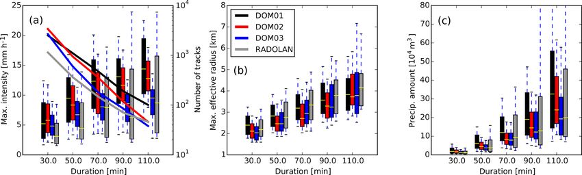
C. Moseley et al.: Impact of resolution on large-eddy simulation                                                                              2899

Figure 5. Life cycles of track composites (including the days 29 May, 3 June, and 6 June) for solitary tracks of different track duration for
model results in three domains with 625 m (DOM01), 312 m (DOM02), and 156 m (DOM03) grid spacings and for radar results. Curves show
mean track life cycles of area-mean precipitation intensity (a–c), area of precipitation objects (d–f), and rate of total precipitation (that is the
areal integral of local precipitation intensity over the object extent) (g–i), conditioned on tracks with durations between 20 and 40 min (a, d,
g), between 50 and 70 min (b, e, h), and between 80 and 100 min (c, f, i).

4     Analysis of the continuous 36 d period with 625 m                     is slightly overestimated, like on 19 and 26 June. Another
      grid spacing                                                          mismatch between model and radar data is that daily peak
                                                                            intensities tend to be reached 1–3 h earlier in the model sim-
4.1    Mean diurnal cycles                                                  ulation compared to RADOLAN. This is particularly visible
                                                                            in the 6 d period of 3–8 June. This feature can be explained
In the previous section we argued that the ICON-LEM setup                   by the observation discussed in the Sect. 3, where we argued
with 625 m grid spacing is sufficient to reasonably simu-                   that convection is triggered too fast in the 625 m LES. We
late typical convective summer days over Germany, although                  note that in addition to these systematic differences, some of
there may still be room for added value at even higher res-                 the differences between model and radar data could also be
olutions. We now discuss the continuous simulation period                   traced back to the uncertainty in boundary conditions from
from 26 May until 20 June 2016, simulated with 625 m grid                   the COSMO forecast data.
spacing. The simulated domain mean precipitation with the                      To confirm that the simulated 36 d convective period is
RADOLAN data for the full period is shown in Fig. 7. On                     long enough to show the intensification of convection with
some of the days we see an underestimation of simulated                     higher temperatures as discussed in the introduction and that
rainfall compared to RADOLAN, like on 30 May, 12 June,                      it is also simulated with ICON-LEM and 625 m grid spac-
and 16 June and in the 3 d period between 23 and 25 June.                   ing, we perform a separate analysis for selected cool and
However, there are few days where the precipitation intensity

www.atmos-chem-phys.net/20/2891/2020/                                                           Atmos. Chem. Phys., 20, 2891–2910, 2020
2900 C. Moseley et al.: Impact of resolution on large-eddy simulation Figure 6. Box-and-whisker plots showing the statistics of solitary tracks, including the days 29 May, 3 June, and 6 June in all three domains with 625 m (DOM01), 312 m (DOM02), and 156 m (DOM03) grid spacing and for the radar data. Values of track maximum intensity (a), track maximum effective radius (b), and total precipitation amount produced by the individual tracks (c) are conditioned on track duration ranging between 20 and 120 min, in five bins of 20 min width. Boxes indicate the 25th and 75th percentiles, and the median (yellow bar), whiskers indicate the 10th and 90th percentiles. The number of tracks in each bin is indicated by the solid lines in panel (a) (note the logarithmic axis on the right). Figure 7. Time series of the mean precipitation intensity P for the 625 m grid spacing ICON-LEM simulation, and the RADOLAN-derived precipitation intensity, for the full 36 d period from 26 May until 30 June 2016. Note that the time series was broken into the upper and the lower panels. Averaging was carried out over all grid boxes where radar data are available. warm days. We calculate the domain mean temperature from Mean diurnal cycles of several domain-averaged quanti- the original COSMO-DE forcing data, and we average over ties, including all 36 d, and conditioned on cool and warm the time between 08:00 and 20:00 UTC when daytime con- days are shown in Fig. 8. As already mentioned, the peak vection is expected. We hereby use the original COSMO- in mean precipitation (Fig. 8a) appears earlier in the model DE analysis data that provided the forcing, as we expect than in the RADOLAN data, and it is higher for the cold them to be closer to the actual temperatures than the tem- days than for the total mean of all days. For warm days, peratures simulated by ICON-LEM. We classify days below the peak is also slightly larger than for the total mean, al- 16 ◦ C daytime mean 2 m temperature as cool and between 19 though there is less precipitation in the afternoon hours af- and 21 ◦ C as warm. The 2 exceptionally warm days 23 and ter 15:00 UTC. The simulation period is too short to signif- 24 June with mean temperatures of 26.0 and 24.1 ◦ C, respec- icantly state if there is any direct correlation between the tively, are not included in the ensemble of warm days. Fur- total amount of precipitation and the daily mean tempera- ther, 22 June was removed from the classification due to the ture. However, there is clear temperature dependence of the very low precipitation amount (otherwise it should have been 99th percentile of precipitation intensity (Fig. 8b): consistent classified as a warm day). An overview of the classified days with the CC argument mentioned in the introduction, there can be seen in Table A1. In total, out of the 36 d of the simu- is less (more) water vapor available in the atmosphere on lation, we classify 6 d as cool and 6 d as warm. cool (warm) days than on average (Fig. 8c), associated with Atmos. Chem. Phys., 20, 2891–2910, 2020 www.atmos-chem-phys.net/20/2891/2020/
C. Moseley et al.: Impact of resolution on large-eddy simulation 2901
Figure 8. Diurnal cycles of mean precipitation intensity (a), 99th percentile of precipitation intensity (b), water vapor path (c), air temperature
at 2 m (d), surface latent heat flux (e), and surface sensible heat flux (f), for all days, cold days, and warm days of the 36 d simulation with
625 m grid spacing. In panels (a) and (b), solid lines show simulation data, and dashed lines show RADOLAN data. Averaging was carried
out over all grid boxes where radar data are available.
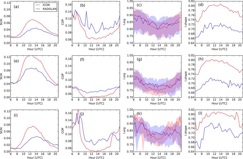
lower (higher) extreme rainfall intensities. However, the dif- degree of organization revealed by RADOLAN (Fig. 9a–b)
ferences in the 99th percentile of precipitation are more pro- and produces more rounded objects than the radar observa-
nounced in the RADOLAN data, suggesting that the sensitiv- tions (Fig. 9d), especially in the afternoon, as was discussed
ity of heavy rainfall to temperature is underestimated by the in Sect. 3.2.
model. Further, we see that cool (warm) days are associated For the 6 cool days, SCAI is in general larger, while COP
with lower (higher) surface fluxes (Fig. 8d–f). As a sensitiv- is lower than the corresponding indices for the 36 d period
ity test, we randomly chose 3 out of the 6 warm days and 3 (Fig. 9e, f), indicating the presence of more numerous and
out of the 6 cool days, and we reproduced the plot in Fig. 8b smaller objects. Although the degree of organization of these
with these days (not shown). Repeating this procedure four objects is weaker than for the full period (Fig. 9e–g), the vari-
times confirmed that peak intensities of the 99th percentiles ability in the shape (Fig. 9h) is similar to that in the larger
are stronger (weaker) for warm (cool) days in both radar and period. In contrast to the cool days, during the 6 warm days,
model data and that the difference between warm and cool SCAI and COP show a diurnal cycle similar to that of the
days is weaker in the model than in the radar data. 36 d period (Fig. 9i, j), revealing the presence of fewer and
larger objects, which favors organization. Iorg also indicates a
4.2 Diurnal cycles of convective organization indices stronger degree of organization (Fig. 9k) in comparison with
the cool days. Although Ishape is noisier on warm days, it
We calculate mean diurnal cycles of the convective organi- also follows a behavior similar (Fig. 9l) to that seen during
zation indices SCAI, COP, Iorg , and Ishape , for model and the longer period.
RADOLAN data of all 36 d and conditioned on cool and Overall, although the indices hint at an underrepresenta-
warm days (Fig. 9). SCAI, COP, and Iorg indicate more orga- tion of convective organization and more compact objects in
nization in the morning and evening, when the objects also the 625 m LES, the radar and model agree that organization
present a more elliptical shape (Fig. 9d). During the after- is stronger on warmer days. However, there is a less clear
noon, when the convective activity is more intense, there is signal for the warm days compared to the average than for
a decrease in the degree of organization, with the shape of the cool days.
the objects tending towards a more circular one. ICON re-
produces the diurnal cycle of Iorg very well (Fig. 9c). Al-
though the variability of SCAI, COP, and Ishape is captured
by the model at 625 m grid spacing, it underestimates the
www.atmos-chem-phys.net/20/2891/2020/ Atmos. Chem. Phys., 20, 2891–2910, 20202902 C. Moseley et al.: Impact of resolution on large-eddy simulation
Figure 9. Mean diurnal cycles of the convective organization indices SCAI (a, e, i), COP (b, f, j), Iorg (c, g, k; color shading shows the
range between percentiles 2.5 and 97.5 as described in Sect. 2.4), and Ishape (d, h, l), for all days (a–d), for cool days (e–h), and for warm
days (i–l), for the model simulation with 625 m grid spacing and for RADOLAN. Averaging was carried out over all grid boxes where radar
data are available.
Table 2. Ratio of the number of tracks of given track types (solitary, tracks that involve only merging, tracks that involve only splitting and
tracks involving both merging and splitting), and the total amount of rainfall that they contribute, relative to the total number and rainfall
amount of all tracks. Tracks that touch the domain boundaries are removed from the analysis. Fractions (in percent), including all 36 model
days, and conditioned on only the cold and the warm days, as defined in Table A1, are given for both the model simulation (M) and the
RADOLAN composite (R).
Ratio (number; amount) (%) All days (M) Cool days (M) Warm days (M) All days (R) Cool days (R) Warm days (R)
Solitary tracks 38.8; 12.1 35.5; 11.9 39.1; 13.6 29.8; 5.1 26.5; 4.1 35.7; 8.4
Involving only merging 23.1; 27.0 23.8; 27.4 24.1; 28.7 27.8; 25.1 28.9; 25.1 26.9; 28.5
Involving only splitting 27.1; 26.5 28.6; 28.3 27.1; 25.6 27.6; 24.2 28.7; 23.1 25.2; 27.8
Both merging and splitting 11.0; 34.4 12.1; 32.4 9.7; 32.1 14.8; 25.6 15.8; 47.7 12.1; 35.3
4.3 Track statistics precipitation produced by solitary tracks and that this trend is
the same for model and RADOLAN data: there is a smaller
fraction of solitary tracks on the cold days and a larger one
We have shown in Sect. 3.3 that in addition to the four con- on the warm days, compared to the full simulation period.
vective organization indices, the rain cell tracking result pro- Likewise, the solitary tracks contribute to a fraction of total
vides information on the degree of organization in the three rainfall that is smaller on cold days but larger on warm days.
different model resolutions. In this section we apply the rain This trend is weaker in the model than in the radar data. At
cell tracking in a similar way on the 36 d continuous simula- first glance, this result seems to contradict our analysis of the
tion with 625 m grid spacing with a separate analysis for the 3 three-domain days, where we argued that a larger contri-
6 cool days and 6 warm days. Table 2 shows that there is a bution of solitary tracks corresponds to a weaker degree of
consistent trend in the ratio of both the number and the total
Atmos. Chem. Phys., 20, 2891–2910, 2020 www.atmos-chem-phys.net/20/2891/2020/C. Moseley et al.: Impact of resolution on large-eddy simulation 2903 organization: instead, the organization indices in Fig. 9 show RADOLAN. Furthermore, a larger number of solitary tracks weaker organization on the cold days, although the contribu- on cool days in both model and RADOLAN data is consis- tion of solitary tracks is smaller, meaning that a larger frac- tent with a weaker degree of convective organization. tion of tracks are subject to merging or splitting events. How- ever, it should be kept in mind that there was also more total precipitation in the analysis domain on the cool days com- 5 Discussion pared to the total simulation period (Fig. 7), which is also reflected by the total number of tracks: while there are on av- We have evaluated the impact of horizontal resolution on ex- erage 21 533 solitary tracks per day for the full model period, plicitly simulated convective precipitation, and we analyzed the number of solitary tracks per day for the cold days was the sensitivity of convective organization to daily mean 2 m 33 367 and therefore in total larger, while for the warm days air temperature on the 36 d continuous simulation with 625 m there was a smaller number of only 20 010 solitary tracks per grid spacing. The impact of horizontal resolution is signifi- day. For the RADOLAN data, these numbers were 8882 (all cant. Our study indicates that compared to the RADOLAN days), 17 288 (cool days), and 9024 (warm days). Therefore, data, the diurnal cycles, life cycles, and degree of convective model and RADOLAN data agree on a larger total number organization are simulated better at the innermost nest with of solitary tracks for the 6 cool days, in consistency with the 156 m horizontal grid spacing. This is in agreement with pre- hypothesis that a weaker organization on the cool days is as- vious studies which argued that for a sufficient resolution of sociated with a larger number of non-interacting rain cells. the processes within deep convective updrafts, models with That the solitary track ratio with respect to the total num- grid spacing of the order of ca. 100 m are required (Petch ber of all tracks is slightly smaller on the cool days could et al., 2002; Bryan et al., 2003) and that there is neither be due to the fact that the larger number of precipitation ob- bulk convergence nor structural convergence at coarser res- jects (as indicated by the SCAI and COP indices) makes it olutions (Panosetti et al., 2019). At 625 m and to a smaller more likely that neighboring objects interact with each other. degree at 312 m grid spacing, convection tends to set in too This phenomenon was observed in the idealized LES study rapidly, and many isolated deep convective cells are scattered by Moseley et al. (2019) where model simulations with more over the domain. In contrast, at 156 m, we find a smoother convective rainfall and a larger number of rain cells showed a onset of convective updrafts with lower peak intensities and a larger contribution of interacting rain cells to the total precip- stronger degree of organization that in general shows a better itation. We note that due to the large differences in the total match with the radar data. In addition, the tracking analysis number of tracks between warm and cool days, the track- revealed that the stronger organization of the more highly re- ing statistics are more difficult to interpret here, compared to solved simulations is accompanied by an increased tendency the more robust differences in track statistics between reso- of convection to form larger clusters: the 156 m simulation lutions presented in Sect. 3.3. shows a lower number of isolated rain cells, and their contri- The box-and-whisker plots in Fig. 10 show the statistics bution to total rainfall is lower. Vice versa, the total contribu- of maximum track intensities, maximum cell radii, and to- tion of the tracks that undergo merging and splitting is clearly tal precipitation amount of the solitary tracks. The solid lines higher for the more highly resolved simulations. Petch et al. in Fig. 10a–c show that the abovementioned larger number (2002) argue that at coarser resolutions the models fail to of solitary tracks per day of the cold days (Fig. 10b) is dis- compensate for the lack of resolved transport out of the sub- tributed over all track durations. Compared to the total en- cloud layer, leading to a delayed spin-up of convection rela- semble of all 36 d, a smaller (larger) fraction of solitary tracks tive to that obtained in the better-resolved simulations. This reach higher maximum intensities on cool (warm) days, and delay in the spin-up might then lead to the too explosive con- in consistency with the 99th percentile of rain intensities vective initiation that we find in our analysis. We speculate shown in Fig. 7b there is a weaker temperature sensitivity that this could also be the reason for the suppressed organi- seen for the model data compared to RADOLAN. This inten- zation of the 625 m simulation compared to radar: as soon as sification of the solitary tracks with temperature, especially a convection cell is initiated, it is already fully developed and for the tracks with a lifetime longer than 1 h, can be seen therefore does not have enough time to interact with neigh- even more clearly in the total amount of precipitation pro- boring cells within its lifetime. However, this is a hypothesis duced by the tracks (Fig. 10g–i). A dependence of the cell that should be tested in a future study. Such a study should sizes reached by solitary tracks in temperature is less clear investigate the processes that happen within merging cells in (Fig. 10d–f). more detail. To briefly summarize the tracking result in this paragraph, An improved subgrid scheme might lead to more realis- we find that solitary tracks of comparable duration can reach tic results and a decreased sensitivity to resolution, while the higher precipitation amounts on warm days compared to Smagorinsky subgrid scheme used in our model seems to not cool days. This shows an intensification of solitary convec- be the optimal choice at 625 m grid spacing, as some of the tive rain tracks with temperature. However, this intensifica- larger boundary-layer eddies are likely unresolved. We also tion is found to be weaker for the model data compared to note that the microphysics scheme might have significant im- www.atmos-chem-phys.net/20/2891/2020/ Atmos. Chem. Phys., 20, 2891–2910, 2020
You can also read