Asymmetric Ensemble of Asymmetric U-Net Models for Brain Tumor Segmentation With Uncertainty Estimation
←
→
Page content transcription
If your browser does not render page correctly, please read the page content below
ORIGINAL RESEARCH
                                                                                                                                          published: 30 September 2021
                                                                                                                                         doi: 10.3389/fneur.2021.609646

                                               Asymmetric Ensemble of
                                               Asymmetric U-Net Models for Brain
                                               Tumor Segmentation With
                                               Uncertainty Estimation
                                               Sarahi Rosas-Gonzalez 1 , Taibou Birgui-Sekou 2 , Moncef Hidane 2 , Ilyess Zemmoura 1 and
                                               Clovis Tauber 1*
                                               1
                                                 UMR Inserm U1253, iBrain, Université de Tours, Inserm, Tours, France, 2 LIFAT EA 6300, INSA Centre Val de Loire,
                                               Université de Tours, Tours, France

                             Edited by:        Accurate brain tumor segmentation is crucial for clinical assessment, follow-up, and
                          Fabien Scalzo,       subsequent treatment of gliomas. While convolutional neural networks (CNN) have
  University of California, Los Angeles,
                           United States
                                               become state of the art in this task, most proposed models either use 2D architectures
                        Reviewed by:
                                               ignoring 3D contextual information or 3D models requiring large memory capacity and
                            Fan Zhang,         extensive learning databases. In this study, an ensemble of two kinds of U-Net-like
             Harvard Medical School,
                                               models based on both 3D and 2.5D convolutions is proposed to segment multimodal
                         United States
                      Yoshinobu Sato,          magnetic resonance images (MRI). The 3D model uses concatenated data in a modified
         Nara Institute of Science and         U-Net architecture. In contrast, the 2.5D model is based on a multi-input strategy
          Technology (NAIST), Japan
                                               to extract low-level features from each modality independently and on a new 2.5D
                   *Correspondence:
                         Clovis Tauber
                                               Multi-View Inception block that aims to merge features from different views of a 3D
            clovis.tauber@univ-tours.fr        image aggregating multi-scale features. The Asymmetric Ensemble of Asymmetric
                                               U-Net (AE AU-Net) based on both is designed to find a balance between increasing
                    Specialty section:
          This article was submitted to
                                               multi-scale and 3D contextual information extraction and keeping memory consumption
                Applied Neuroimaging,          low. Experiments on 2019 dataset show that our model improves enhancing tumor
                a section of the journal
                                               sub-region segmentation. Overall, performance is comparable with state-of-the-art
                 Frontiers in Neurology
                                               results, although with less learning data or memory requirements. In addition, we provide
         Received: 31 October 2020
             Accepted: 22 July 2021            voxel-wise and structure-wise uncertainties of the segmentation results, and we have
      Published: 30 September 2021             established qualitative and quantitative relationships between uncertainty and prediction
                             Citation:         errors. Dice similarity coefficient for the whole tumor, tumor core, and tumor enhancing
   Rosas-Gonzalez S, Birgui-Sekou T,
 Hidane M, Zemmoura I and Tauber C
                                               regions on BraTS 2019 validation dataset were 0.902, 0.815, and 0.773. We also applied
      (2021) Asymmetric Ensemble of            our method in BraTS 2018 with corresponding Dice score values of 0.908, 0.838,
  Asymmetric U-Net Models for Brain            and 0.800.
Tumor Segmentation With Uncertainty
Estimation. Front. Neurol. 12:609646.          Keywords: brain tumor segmentation, deep-learning, BraTS, multi-input, multi- view, inception, uncertainties, 2.5D
     doi: 10.3389/fneur.2021.609646            convolutions

Frontiers in Neurology | www.frontiersin.org                                         1                                      September 2021 | Volume 12 | Article 609646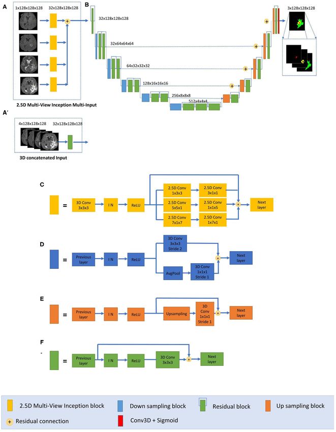
Rosas-Gonzalez et al.                                                                                        AEAU-Net for Brain Tumor Segmentation

INTRODUCTION                                                              that can be used (23). Consequently, the use of 2D convolutions
                                                                          for slice-by-slice segmentation is also a common practice that
Glioma is the most frequent primary brain tumor (1). It has its           reduces memory requirement (24). Multi-view approaches have
origin in glial cells and can be classified into I to IV grades,          also been developed to address the same problem. McKinley
depending on phenotypic cell characteristics. In this grading             et al. (18) and Xue et al. (25) showed that applying 2D
system, low-grade gliomas (LGGs) correspond to grades I and               networks in axial, sagittal, and coronal views and combining their
II, whereas high-grade gliomas (HGGs) are grades III and IV.              results can recover 3D spatial information. Recently, one of the
The primary treatment is surgical resection followed by radiation         top-performing submissions in the BraTS 2019 challenge (20)
therapy and/or chemotherapy.                                              proposed a hybrid model that goes from 3D to 2D convolutions
    MRI is a non-invasive imaging technique commonly used                 extracting two-dimensional features in each of the orthogonal
for diagnosis, surgery planning, and follow-up of brain tumors            planes and then combines the results in an ensemble model.
due to its high resolution on brain structures. Currently,                Wang et al. (16) demonstrated that using three 2.5D networks
tumor regions are segmented manually from MRI images by                   to obtain separate predictions from three orthogonal views and
radiologists, but due to the high variability in image appearance,        fusing them at test time can provide more accurate segmentations
the process is very time consuming and challenging, and                   than using an equivalent 3D isotropic network. While they
inter-observer reproducibility is considerably low (2). Since             require the training and optimization of several models, ensemble
accurate tumor segmentation is determinant for surgery, follow-           models are currently the top-performing methods for brain
up, and subsequent treatment of glioma, finding an automatic              tumor segmentation.
and reproducible solution may save time for physicians and                    On the other hand, some strategies have been implemented
contribute to improving the clinical assessment of glioma                 to aggregate multi-scale features. Cahall et al. (26) showed
patients. Based on this observation, the Multimodal Brain                 a significant improvement in brain tumor segmentation by
Tumor Segmentation Challenge (BraTS) aims at stimulating                  incorporating Inception blocks (27) into a 2D U-Net architecture.
the development and the comparison of the state-of-the-art                Wang et al. (16) and McKinley et al. (20) used dilated
segmentation algorithms by making available an extensive pre-             convolutions (28) in their architecture with the same aim of
operative multimodal MRI dataset provided with ground truth               obtaining both local and more global features. While significant,
labels for three tumor tissues: enhancing tumor, the peritumoral          aggregating multi-scale features is limited by the requirement
edema, and the necrotic and non-enhancing tumor core.                     of more memory capacity. To address this, the use of Inception
This dataset contains four modalities: T2-weighted (T2), fluid-           modules has been incorporated into 2D networks (26), not taking
attenuated inversion recovery (FLAIR), T1-weighted (T1), and              advantage of 3D contextual information. In addition, Inception
T1 with contrast-enhancing gadolinium (T1c) (3–7).                        modules have been integrated into a cascade network approach
    Modern convolutional neural networks (CNNs) are currently             (29). The model first learns the whole tumor, then the tumor core,
state-of-the-art in many medical image analysis applications,             and finally the enhancing tumor region. This method requires
including brain tumor segmentation (8). CNNs are hierarchical             three different networks and thus increases the training and
groups within filter banks that extract increasingly high-level           inference time. Another approach to extract multi-scale features
image features by feeding the output of each layer to the next            uses dilated convolutions. This operation was explicitly designed
one. Recently, Ronneberger et al. (9) proposed an effective U-Net         for semantic segmentation and tackled the dilemma of obtaining
model, a fully convolutional network (FCN) encoder/decoder                multi-scale aggregation without losing full resolution, increasing
architecture. The encoder module consists of multiple connected           the receptive field (28). Wang et al. (16) and McKinley et al. (20)
convolution layers that aim to gradually reduce the spatial               implemented different dilation rates in sequential convolutions;
dimension of feature maps and capture high-level semantic                 nevertheless, it has not been used to extract multi-scale features
features appropriate for class discrimination. The decoder                in a parallel way in a single layer and, if not applied carefully, can
module uses upsampling layers to recover the spatial extent               cause gridding effects, especially in small regions (30).
and object representation. The main contribution of U-Net is                  In terms of accuracy and precision, the performance of
that, while upsampling and going deeper into the network,                 CNNs are currently comparable with human-level performance
the model concatenates the higher resolution features from the            or even better in many medical image analysis applications
encoder path with the upsampled features in the asymmetric                (31). However, CNNs have also often been shown to produce
decoder path to better localize and learn representations in              inaccurate and unreliable probability estimates (32, 33). This
following convolutions. The U-Net architecture is one of the              has drawn attention to the importance of uncertainty estimation
most widely used for brain tumor segmentation, and its versatile          in CNN (34). Among other advantages, the measurement of
and straightforward architecture has been successfully used               uncertainties would enable knowing how confident a method is
in numerous segmentation tasks (10–14). All top-performing                in implementing a particular task. This information can facilitate
participants in the last two editions of the BraTS challenge used         CNN’s incorporation into clinical practice and serve the end-user
this architecture (15–22).                                                by focusing attention on areas with high uncertainty (35).
    While 3D CNN can provide global context information of                    In this study, we propose an approach that addresses a
volumetric tumors, the large size of the images makes the use             current challenge of brain tumor segmentation, keeping reduced
of 3D convolutions very memory demanding, which limits the                memory requirements while benefiting from multi-scale 3D
patches and batch size, as well as the number of layers and filters       information. To do so, we propose an ensemble model, called

Frontiers in Neurology | www.frontiersin.org                          2                                 September 2021 | Volume 12 | Article 609646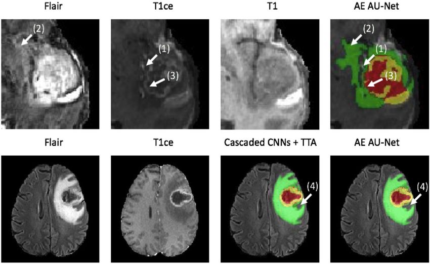
Rosas-Gonzalez et al.                                                                                      AEAU-Net for Brain Tumor Segmentation

Asymmetric Ensemble Asymmetric U-Net (AE AU-Net), based                   using a concatenation operation. This enables reducing memory
on an Asymmetrical 3D residual U-Net (AU-Net) using two                   consumption while maintaining similar performances compared
different kinds of inputs: (1) concatenated multimodal 3D MRI             with using concatenation operations. Finally, each level of the
data (3D AU-Net) and (2) a 2.5D Multi-View Inception Multi-               encoding pathway consists of two residual blocks (green blocks
Input module (2.5D AU-Net). The proposed AU-Net is wider in               in Figure 1) followed by a downsampling block (blue blocks). We
the encoding path to extract more semantic features, has residual         used convolutions with stride equal to 2 for downsizing image
blocks in each level to increase training speed, and additive skip        dimension, maintaining the same number of filters in the first
connections between the encoding and decoding path instead of             two levels and then increasing the number of features in each
a concatenation operation to reduce the memory consumption.               level with an initial number of filters equal to 32. Thus, the
The proposed 2.5D strategy allows us to extract low-level features        spatial dimension of the initial training patches of size 128 ×
from each modality independently. In this way, the model can              128 × 128 was reduced by a factor of 32 in the encoding path.
retrieve specific details related to tumor appearance from the            In the decoding path, we used only one residual block in each
most informative modalities, without the risk of being lost when          level, and we used upsampling layers, which duplicate values in a
combined during the downsampling. The Multi-View Inception                sliding window to increase the dimension. The upsampling layers
block aims to merge features from both different views and                are directly followed by convolution ones. This technique of
different scales simultaneously, seeking a balance between 3D             upsampling helps to avoid the checkerboard pattern generated by
information usage and memory footprint. In addition, we use an            transposed convolution (deconvolution) layers as experimented
ensemble of models to improve our segmentation results and the            by Odena et al. (38).
generalization power of our method and also as a way to measure               The final activation layer uses a sigmoid as an activation
epistemic uncertainty and estimate structure-wise uncertainty.            function to output three prediction maps of the same size as
                                                                          the initial training patches into three channels corresponding to
                                                                          the regions: whole tumor, tumor core, and enhancing tumor.
METHODS                                                                   We chose to classify the three regions by doing three binary
Network Architecture                                                      classifications, one for each region.
We have developed a modified U-Net architecture with five-level
asymmetric descending and ascending parts implemented with                3D AU-Net
two kinds of inputs for ensemble modeling (Figure 1). While the           The proposed AU-Net was used with two different kinds of
first input is a classical concatenation of 3D MRI data, the second       inputs. In the first one, called 3D AU-Net, 3D concatenated MRI
one is a novel 2.5D Multi-View Inception Multi-Input module               sequences are used as the input to capture classical multimodal
aiming to extract low-level textural features of the tumor. Details       information from the different MRI sequences. This input is
of the modified U-Net proposed inputs and assembling strategy             presented in Figure 1A′ .
are provided.
                                                                          2.5D AU-Net
Asymmetric U-Net (AU-Net)                                                 The second type of input is proposed to capture the textural
The main component of our network is a modified 3D U-                     and multi-scale features of the tumor better. This second input
Net architecture of five levels (Figure 1B). Traditional 3D U-            is a 2.5D input for the AU-Net, with a different strategy. A
Net architecture has a symmetrical decoder and encoder paths.             multi-input module (Figure 1A) has been developed to maximize
The first path is associated with the extraction of semantic              learning from independent features associated with each
information to make local predictions, while the second section           imaging modality before merging into the encoding/decoding
is related to the recovery of the global structure. AU-Net is             architecture, thus avoiding the loss of specific information
wider in the encoding path than in the decoding path, to extract          provided by each modality. While most previous architectures
more semantic features while keeping memory usage lower. We               concatenate all the MRI modalities as a single multi-channel
added twice more convolutional blocks in the encoding path                input, we propose to extract low-level features associated with
than in the decoding section to achieve this. The standard U-Net          tissue appearance from each modality independently. To do
architecture also does not get enough semantic information in the         so, we divide the input into four paths, one for each imaging
downsampling path because of the limited receptive fields. We             modality, to extract features from each modality independently,
added parallel paths with convolutions with two different filter          and then we merge them as an input of the proposed AU-Net.
sizes in the downsampling blocks (Figure 1D).                                 In addition, we propose that each of these four paths
   This architecture uses residual blocks (Figure 1F) instead             contains what we define as a 2.5D Multi-View Inception module
of a simple sequence of convolutions. The residual blocks                 (Figure 1C) that allows the extraction of features in the different
(36) are obtained by a short skip connection and element-                 orthogonal views of the 3D image: axial, coronal, and sagittal
wise addition operation between each block’s input and output             planes and different scales, merging them all in each forward pass.
feature maps. This simple algorithm does not add additional                   The design of the 2.5D Multi-View Inception module is
training parameters to the network, and it has been shown to              inspired by the Inception module of GoogLeNet (39). Unlike
be beneficial for faster convergence, reducing training time (37).        the Inception module, we use 2.5D anisotropic filters instead
We also used additive skip connections between the encoding               of 3D or 2D isotropic filters, and we add all the resulted
outputs and decoding feature maps of equivalent size instead of           feature maps instead of stacking them. This module has two

Frontiers in Neurology | www.frontiersin.org                          3                                September 2021 | Volume 12 | Article 609646
Rosas-Gonzalez et al.                                                                                                        AEAU-Net for Brain Tumor Segmentation

 FIGURE 1 | Proposed 2.5D Asymmetric U-Net and 3D Asymmetric U-Net. (A) 2.5D Multi-View Inception Multi-input. (A′ ) 3D concatenated input. (B) An asymmetric
 3D U-Net architecture using residual blocks, instance normalization (IN), and additive skip connections between encoding and decoding sections. (C) 2.5D Multi-View
 Inception block. (D) Down sampling block. (E) Up sampling block. (F) Residual block.

Frontiers in Neurology | www.frontiersin.org                                     4                                      September 2021 | Volume 12 | Article 609646
Rosas-Gonzalez et al. AEAU-Net for Brain Tumor Segmentation
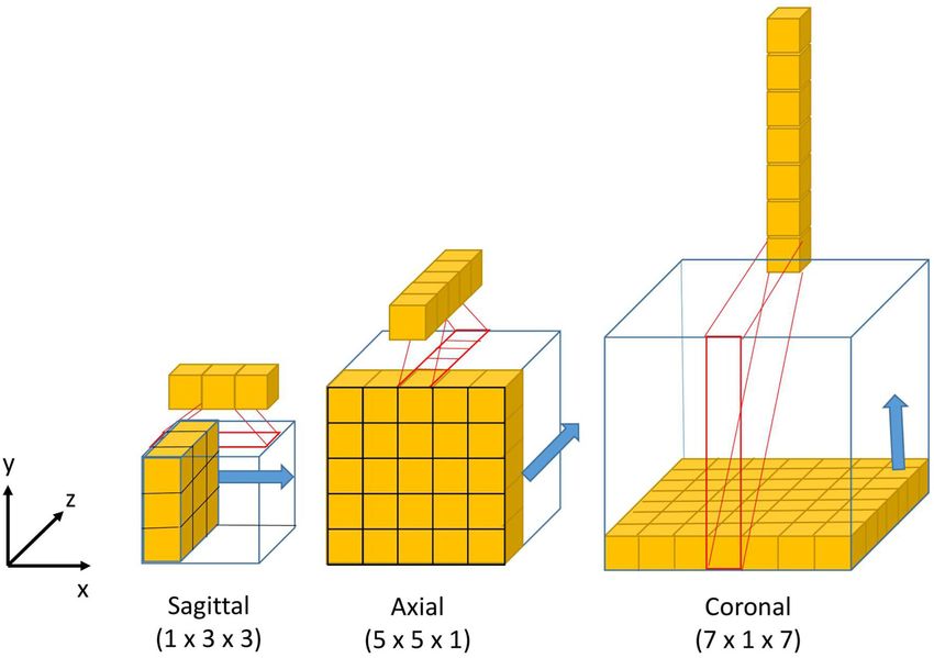
main characteristics: the first one is the use of convolutions (>12 GB GPU). Therefore, our model’s design aims to extract
with different receptive field orientation on each image plane— volumetric information using 2.5D Multi-view filters and multi-
axial, sagittal, and coronal planes—by using anisotropic kernels scale information by training a single network. Training a
oriented in each direction. The second is the fusion of the single network instead of three networks, one for each view as
features extracted using anisotropic kernels at different scales. implemented in (16, 18) should save training time. Our models
Figure 2 shows the way these two characteristics are combined take around 8 h to be trained.
by replacing a typical 3D isotropic convolution 3 × 3 × 3 into
an anisotropic convolution 1 × 3 × 3 followed by a 3 × 1 × Asymmetric Ensemble of Asymmetric U-Net
1 convolution. These filters extract features in the sagittal view (AE AU-Net)
of the image; the same idea is repeated in “y” and “z” directions Since 2017 where Kamnitsas et al. (17) won the BraTS
but using different scales: 5 × 5 × 1 extracts features in the axial challenge using an ensemble of five models with three different
plane and 7 × 1 × 7 in the coronal plane. With this approach, architectures, trained with varying functions of loss and using
the network extracts and merges features from different planes at different normalization techniques, all the winners of the
the same time, with three parallel branches of anisotropic kernels. following competitions have used ensembles of models as a
After each pair of convolutions, an instance normalization (40) strategy to improve the segmentation results of their best single
and ReLU (41) activations are applied. models (15, 19–22). Combining different models reduces the
Our model has been optimized using 2.5D convolutions to influence of hyper-parameter choices and the risk of overfitting,
fit a 12GB GPU memory. 2.5D filters store more weight factors and it is currently the most effective approach for brain
than 2D filters and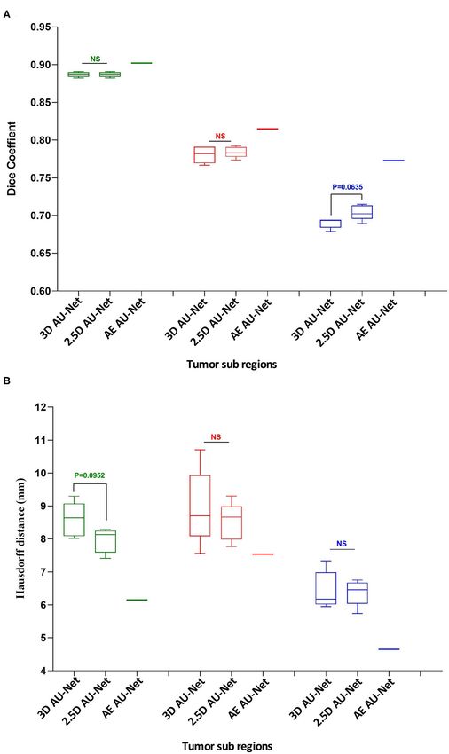
Rosas-Gonzalez et al.                                                                                      AEAU-Net for Brain Tumor Segmentation

segmentation results and the generalization power of our                  anisotropic resolution. All the images were re-sampled and zero-
method by reducing the risk of overfitting. Considering the               padded to the same isotropic resolution (1.0 × 1.0 × 1.0 mm)
different nature of the input data, we call the proposed method           and zero-padded to have the same spatial dimensions (240 × 240
Asymmetric Ensemble of Asymmetric U-Net (AE AU-Net). The                  × 155 mm). Skull-stripping was also performed using the Brain
proposed ensemble model is based on the training of seven                 Extraction Tool (BET) (45) from the FSL (46).
models. According to a 5-fold cross-validation strategy, both                Even though the images provided were already preprocessed
the 3D AU-Net and the 2.5D AU-Net were trained five times                 to homogenize the data (4), image intensity variability can still
each with different subsets of the dataset and varying weights of         negatively impact the learning phase; contrarily to some other
initialization. The seven best-performing models were selected;           imaging techniques like CT, MRI does not have a standard
we finally chose four from 3D AU-Net and three from 2.5D AU-              intensity scale. Therefore, image intensity normalization is often
Net, this mainly due to memory constrictions. The ensemble was            a necessary stage for model convergence. We chose to normalize
obtained by averaging the output probability estimates of the             the MRI images by first dividing each modality by its maximum
labels for each voxel of the image.                                       value and then by centering and reducing the data to have
                                                                          images with the same zero average intensity and unitary SD. This
                                                                          method is widely used due to its simplicity and good qualitative
Data and Implementation Details                                           performance (19, 21).
BraTS Dataset
We validated our model in the 2019 BraTS dataset, which                   Post-processing
consists of pre-operative MRI images of 626 glioma patients.              We implemented the post-processing of the prediction maps of
Each patient’s MRI images contain four modalities T2-weighted             our proposed model to reduce the number of false positives and
(T2), fluid-attenuated inversion recovery (FLAIR), T1-weighted            enhance tumor detection. A threshold value representing the
(T1), and T1 with gadolinium-enhancing contrast (T1c). All                minimum size of the enhancing tumor region was defined, as
images were segmented manually by one to four raters, following           suggested in Isensee et al. (19), and the label of all the voxels
the same annotation protocol. Experienced neuro-radiologists              of the enhancing tumor region was replaced with one of the
approved their annotations. The data are divided into three sets          necrosis regions when the total number of predicted ET voxels
by the organizers of the BraTS challenge: training, validation, and       was lower than the threshold. The threshold value was estimated
test dataset. The training set is the only one provided with expert       as the one that optimizes the overall performance in this region
manual segmentation and the grading information of the disease.           in the validation dataset. Besides, as proposed by McKinley et al.
The training dataset contains images of 335 patients, of which 259        (20), if our model detects no tumor core, we assume that the
are HGG and 76 are LGG. The validation and test datasets include          detected whole tumor region corresponds to the tumor core. We
the same MRI modalities for 125 and 166 patients, respectively.           have relabeled the region as a tumor core.
   In the training dataset, the ground truth labels are provided
for three tumor tissues: enhancing tumor (ET—label 4), the                Implementation and Training
peritumoral edema (ED—label 2), and the necrotic and non-                 The Dice loss function was used to cope with class imbalances
enhancing tumor core (NCR/NET—label 1). From these classes,               and weighted Dice coefficient (WDC) as the evaluation metrics
we defined the following tumor regions to train our models:               to look for the best-performing model (12). Since ground truth
                                                                          segmentations were only provided for the training dataset, we
• The whole tumor (WT) region. This includes the union of the             randomly selected 20% from the training set as our internal
  three tumor tissues ED, ET, and NCR/NET (i.e., label = 1∪               validation set, taking the same percentage of images from LGG
  2 ∪4).                                                                  and HGG patients. We trained our models using the remaining
• The tumor core (TC) region. This is the union of the ET and             80%. The networks were trained for 100 epochs using patches of
  NCR/NET (i.e., label = 1 ∪4).                                           128 × 128 × 128 and Adam optimizer (47) as a back-propagation
• The enhancing tumor (ET) (i.e., label = 4).                             algorithm, with an initial learning rate of 0.0001 and a batch size
                                                                          of 1. The learning rate was decreased by five if no improvement
Pre-processing                                                            was seen, on the validation set, within 10 epochs. Our model takes
The multimodal scans in the BraTS challenge were acquired                 around 8 h to be trained. Figure 3 shows a representative example
from multiple institutions, employing different clinical protocols,       of the learning curves.
resulting in a non-standardized distribution. The challenge                   We compared different data augmentation strategies to
organizers performed several preprocessing steps to homogenize            prevent overfitting, and the best results were obtained using
the dataset. The images from different MR modalities were first           only random crops and random horizontal axis flipping with a
co-registered to the same anatomical template. The SRI24 multi-           probability of 0.5. Note that the data are augmented on the fly
channel atlas of a normal adult human brain template (42) was             during training.
used. The template was obtained by affine registration using                  All experiments were conducted on a workstation Intel-i7
the Linear Image Registration Tool (FLIRT) (43) developed by              2.20 GHz CPU, 48G RAM, and an NVIDIA Titan Xp 12GB
the Oxford Center for Functional MRI of the Brain (FMRIB)                 GPU. All our models were implemented in Keras (48) 2.2 using
and available in the FMRIB Software Library (FSL) (44). The               the Tensorflow (49) 1.8.0 as a backend. All results obtained on
original images were acquired across different views and variable         the validation dataset of the BraTS challenge were uploaded

Frontiers in Neurology | www.frontiersin.org                          6                                September 2021 | Volume 12 | Article 609646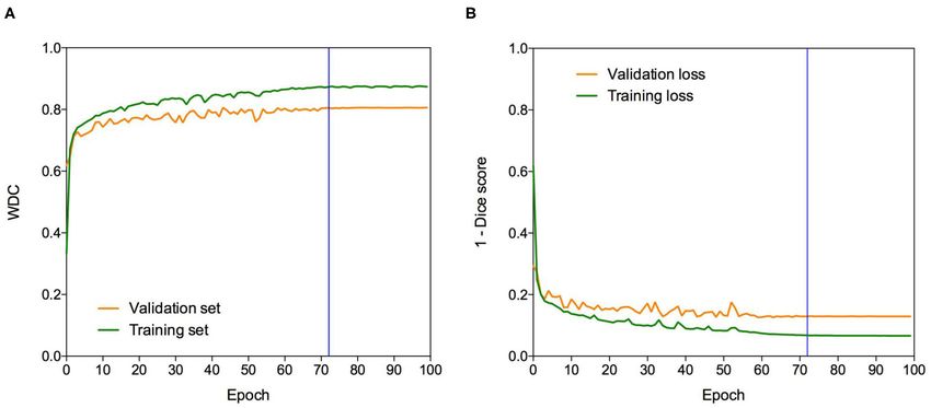
Rosas-Gonzalez et al.                                                                                                       AEAU-Net for Brain Tumor Segmentation

 FIGURE 3 | Learning curves. Example of (A) WDC evaluation metric and (B) (1-Dice score) loss function evolution during training on the BraTS 2019 dataset. The
 blue vertical line shows the moment at which the model reached the best performance in the validation dataset. The best models were obtained systematically before
 the 100 epochs.

on the publicly available evaluation server of BraTS for metrics                     where pc is the sigmoid output average probability of class c and
evaluation. We report the quantitative evaluation values obtained                    C is the set of classes (C = {0, 1} in our case). To measure a
in terms of Dice coefficient and Hausdorff distance, which are                       structure-wise uncertainty, we considered all volumes associated
defined as follows:                                                                  with each region estimated from the ensemble of models. Similar
                                                                                     to Wang et al. (16), we calculated the structure-wise uncertainty
               2 |P ∩ T|                                                             of each region as the volume variation coefficient (VVC):
  Dice (P, T) =          ,                                  (1)
               |P| + |T|
                                                                                                                            σv
                            inf                inf                                                               VVC =         ,                               (4)
 Haus (P, T) = max p ∈ P        d p, t , t ∈ T      d t, p ,                                                                  µv
                           t∈T                 p∈P
                                                                           (2)       where µv and σv are the mean and SD of the N volumes. In this
                                                                                     case, N is equal to seven. Equations (3) and (4) represent the
where P and T are respectively, the set of predicted voxels and                      voxel-wise epistemic uncertainty and structure-wise uncertainty
the ground-truth ones,
                    representing the supremum and inf the                           from the ensemble of models, respectively.
infimum, and d p, t the Euclidian distance between two points
p and t.                                                                             Uncertainty Measure Evaluation
                                                                                     We evaluate our uncertainty estimation method using the metrics
Uncertainty Estimation                                                               proposed in Mehta et al. (50), which were used in the last two
The use of an ensemble of models improves the segmentation                           editions of the BraTS sub-challenge on uncertainty quantification
results and the generalization power. Still, it also allows the                      to rank the participants. The three-selected metrics aim to reward
measurement of epistemic uncertainty and the estimation of                           models when the uncertainty is low in correct predictions and
structure-wise uncertainty that provides additional information                      high in the wrong predictions. In this part of the challenge,
regarding the segmentation results.                                                  participants are required to submit along with the brain tumor
    To estimate epistemic uncertainty, we averaged the model’s                       segmentation, a map of uncertainties associated with each
output probabilities for each label in each voxel to obtain a new                    segmentation. The first metric, the Dice area under the curve
probability measure from the ensemble. Since our model makes                         (Dice AUC), evaluates the Dice score after removing the voxels
a binary classification of each voxel, the highest uncertainty                       with uncertainty levels higher than certain thresholds (0.25, 0.5,
corresponds with a probability of 0.5. Then we used the                              and 0.75). It is expected that removing uncertain voxels will
normalized entropy (Equation 3) to get an uncertainty measure                        increase the segmentation accuracy, but it can also decrease the
of the prediction for each voxel:                                                    Dice score if many correct predictions are removed.
                                                                                        The two other selected metrics are, respectively, the filter true-
                            X         pc log pc                                      positive ratio (FTPR) and the filter true-negative ratio (FTNR),
                  H=−                             ∈ [0, 1] ,               (3)       which aim to penalize the elimination of correct predictions, the
                                c∈C    log (|C|)

Frontiers in Neurology | www.frontiersin.org                                     7                                      September 2021 | Volume 12 | Article 609646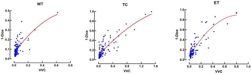
Rosas-Gonzalez et al. AEAU-Net for Brain Tumor Segmentation
true positives (TP) and true negatives (TN), respectively. The to the enhancing tumor, as can be seen in the T1ce image
FTPR is defined as follows: (arrow 1). Comparing our model segmentation qualitatively with
the one reported in Isensee et al. (19), we can say that our model
(TP1.00 − TPτ ) better delimits the region of necrosis and non-enhancing tumor
FTPR = (5)
TP1.00 (in green). Our model overlaps better the hyperintense region
in the FLAIR sequence (arrow 2) but fails to detect the fine
The FTPR at different thresholds (τ ) is measured relative to structures of the enhancing tumor region as signaled (arrow 3).
the unfiltered values (τ = 1.00). The ratio of filtered TN is Our model effectively excludes the blood vessels (arrow 1) from
calculated similarly. the tumor, which are small structures with similar image intensity
The final uncertainty score for each region is calculated to enhancing tumors. Deep learning models usually fail to detect
as follows: such small regions due to the few training examples containing
AUC1 + (1 − AUC2 ) + (1 − AUC3 ) these structures. The use of Dice loss function can explain this
score = , (6) effect, as missing small structures has a low impact on Dice score
3
and, therefore, a low penalization.
which combines the area under the curve of three functions: (1) At the bottom of Figure 5, we compare the segmentation
Dice, (2) FTPR, and (3) FTNR, all as a function of different values made by Wang et al. (51) using cascade networks with test time
of τ . augmentation (cascaded CNNs + TTA) with the one made by
our method for the patient identified as CBICA_ALZ_1. We
Ablation Study can see that our model better segments the necrosis and non-
To evaluate the impact of the proposed AE AU-Net compared enhancing region (arrow 4) but that there are no other significant
with its components, we compared our proposed ensemble differences between the segmentations, resulting in similar Dice
model to two variants: (1) 3D AU-Net, which is the AU-Net scores. This suggests that slight differences in Dice values will
model with concatenated MRI modalities as the input; (2) 2.5D not always represent significant qualitative differences that could
AU-Net, which is the AU-Net with the proposed 2.5D Multi-View impact clinical practice.
Inception Multi-Input as the input.
Quantitative Results
EXPERIMENTS AND RESULTS The corresponding quantitative criteria obtained with the
different approaches are presented in Table 1. For both the
Segmentation Results 3D and 2.5D AU-Net, the results correspond to an ensemble
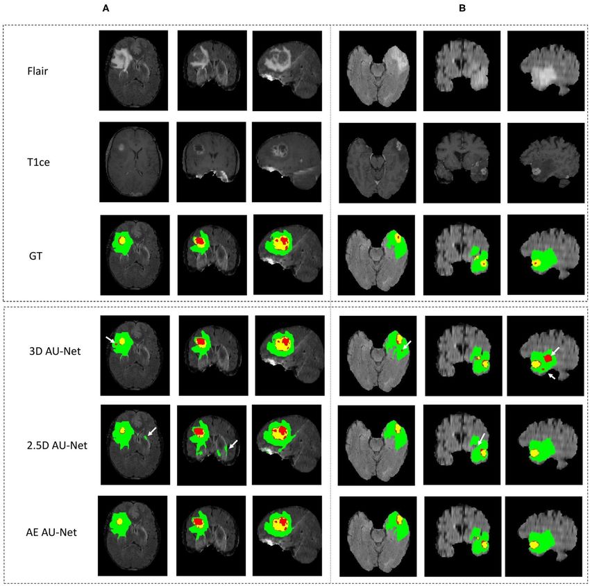
Qualitative Results from 5-fold cross-validation models. Results for all methods
Figure 4 shows an example of segmentation results obtained are presented as averagea ± SD obtained over the BraTS 2019
on two HGG patients with 3D AU-Net, 2.5D AU-Net, and validation dataset. It can be observed that 3D and 2.5D AU-
AE AU-Net. For simplicity of visualization, only the T1ce and Net got relatively similar scores, with better Dice achieved by
FLAIR images are presented. The three orthogonal views, axial, 3D AU-Net on the enhancing tumor, and better Hausdorff
coronal, and sagittal, are displayed for better representation distance obtained by 2.5D AU-Net on the enhancing tumor and
of the volumetric segmentation. The green, yellow, and red tumor core. The proposed AE AU-Net improved all the scores,
regions correspond, respectively, to the whole tumor (WT), the reaching the best values on five criteria out of six, illustrating
enhancing tumor (ET), and the tumor core (TC). The ground that each architecture learned different features to address the
truth provided with the BraTS dataset is presented on the third segmentation problem and complement each other. It achieved
row, followed by 3D and 2.5D AU-Net results on rows 4 and Dice scores of 0.773, 0.902, and 0.815 on the ET, WT, and
5, and the results of the proposed AE AU-Net are presented in TC. For visual comparison, the individual results of the 5-fold
the last row. It can be observed that the segmentation results of cross-validation are presented as box plots in Figure 6, along
the 3D and 2.5D single networks provide proper segmentation, with p-values from Student’s t-test performed to compare the
although with some defects that are highlighted with white different models.
arrows. Looking at the different views and patients, it can be Regarding the Dice metric, no significant difference was
noticed that the performance of the 3D and 2.5D approaches observed between 3D and 2.5D models in the WT and
are varying and that both can present accurate segmentation or TC regions, but a significant difference was observed in the
defects. In contrast, the proposed AE AU-Net appears globally ET region (Figure 6A). Incorporating the 2.5D Multi-View
more accurate, benefiting from both the models to decide more Inception Multi-Input module to the AU-Net improved the result
correctly the labeling of the voxels. in this region compared with 3D input. The best performance
In Figure 5, we present two examples of segmentation made was obtained in all regions with the AE AU-Net, which over-
by our AE AU-Net model ensemble. Both patient images were performed 3D and 2.5D AU-Nets with a statistically significant
taken from the 2018 validation dataset. In the top, we show the difference (p < 0.008). Regarding the Hausdorff distance, it
patient identified as CBICA_AZA_1 in the BraTS dataset. We can be observed that the variability of the results was higher
selected the same example reported in Isensee et al. (19) for compared with the Dice metric (Figure 6B). No statistically
a qualitative comparison. This case example has been reported significant difference was found between 3D and 2.5D models
as a difficult case for segmentation due to blood vessels close in the TC and ET regions. In WT, 2.5D AU-Net obtained
Frontiers in Neurology | www.frontiersin.org 8 September 2021 | Volume 12 | Article 609646Rosas-Gonzalez et al. AEAU-Net for Brain Tumor Segmentation FIGURE 4 | (A,B) Qualitative results. Example of segmentation improvement using our proposed model AE AU-Net in two patients from the BraTS 2019 training dataset. The whole tumor (WT) region includes the union of the three tissues (ED, ET, and NET); the tumor core (TC) region is the union of the necrotic and non-enhancing tumor (red) and enhancing tumor (yellow). a significant improvement with respect to the 3D AU-Net and test datasets, illustrating that the method did not overfit the model. The smaller Hausdorff distances were obtained in the validation dataset and generalized well to the test dataset. three regions with the proposed AE AU-Net with a statistically We have improved the model and the segmentation significant difference (p < 0.008). performance in the validation dataset by implementing the This study has extended our previous work (52), which proposed AE AU-Net as an ensemble of seven asymmetric corresponds to a single model from 2.5D AU-Net architecture. models and using additional post-processing techniques. We Table 2 shows the results of this single model in the validation also implemented our proposed AE AU-Net framework in and test dataset of the BraTS 2019. We can observe that the 2.5D BraTS 2018 for comparison purposes. In Table 3, we compared model achieved a similar overall performance in both validation our implementation on BraTS 2018 with a 3D U-Net (53) Frontiers in Neurology | www.frontiersin.org 9 September 2021 | Volume 12 | Article 609646
Rosas-Gonzalez et al.                                                                                                                  AEAU-Net for Brain Tumor Segmentation

 FIGURE 5 | Qualitative results. Two example segmentations using our proposed ensemble. In the top patient identified as CBICA_ZA_1 and in the bottom the patient
 CBICA_ALZ_1, both from the BraTS 2018 validation dataset. In the bottom, we compare our results with the segmentation made using the Cascaded Networks +
 TTA presented in (51).

TABLE 1 | Ablation study on BraTS validation data (125 cases).

                                                              Dice                                                                   Hausdorff 95 (mm)

                                     ET                        WT                        TC                       ET                         WT                           TC

3D AU-Net (5-CV)               0. 730 ± 0.284            0.895 ± 0.070             0.796 ± 0.186            6.06 ± 10.54                 6.20 ± 9.21                8.40 ± 12.09
2.5D AU-Net (5-CV)             0.714 ± 0.295             0.898 ± 0.066             0.798 ± 0.189             5.74 ± 9.92                 6.79 ± 12.6                 7.46 ± 9.13
AE AU-Net (5-CV)               0.773 ± 0.257             0.902 ± 0.066             0.815 ± 0.161             4.65 ± 8.10                 6.15 ± 11.2                7.54 ± 11.14

Ensemble results from 5-fold cross-validation are reported for 3D, 2.5D, and AE AU-Net models. The online BraTS evaluation platform computed reported metrics. ET, enhancing tumor;
WT, whole tumor; TC, tumor core; 5-CV, ensemble results from 5-fold cross-validation. Bold values highlight the best results for each metric.

reimplemented by (51) and cascaded networks (51). We also                                        Table 4 shows a comparative performance between the
compare our results with the top-performing methods in the                                   proposed AE AU-Net model and the two best-performing
BraTS 2018 challenge, including the first place of the competition                           networks presented to BraTS 2019 (15, 22). It can be observed
(21) and the second place (19). From the comparison with                                     in Table 4 that our method performs closely, although a
cascade networks, we can observe that our method has a similar                               little less, to the second-ranked submission in the validation
performance in terms of Dice in the enhancing tumor and                                      dataset and that our model performs better than the second-
whole tumor regions. We got a comparable although slightly                                   place model in the enhancing tumor region. The difference
lower performance with the top-performing methods in the same                                in performance in both BraTS datasets, 2018 and 2019,
regions, with a lower performance in the tumor core region.                                  could be explained by the fact that the second performer
We got better performance in terms of Hausdorff distance than                                (19) and (15) did not only use the BraTS dataset to train
cascade networks in the ET and in the WT regions and similar                                 their model but also an additional Decathlon dataset (54).
performance with the competition winners.                                                    Regarding the top score (22), it comparatively requires more

Frontiers in Neurology | www.frontiersin.org                                            10                                        September 2021 | Volume 12 | Article 609646
Rosas-Gonzalez et al. AEAU-Net for Brain Tumor Segmentation FIGURE 6 | Quantitative results. Box plot comparing two models in a 5-fold cross-validation: the 3D Asymmetric U-Net, the 2.5D Asymmetric U-Net, and the impact of our proposed model (AE AU-Net). (A) The y-axis presents the Dice score values for the three tumor sub-regions in the x-axis. (B) The y-axis shows the Hausdorff distance for the three tumor sub-regions in the x-axis. In green, red, and blue are depicted the three tumor sub-regions: whole tumor, tumor core, and enhancing tumor. The third column corresponding to our AE AU-Net is not a box plot; it is a single value obtained with the ensemble for comparison purposes. Frontiers in Neurology | www.frontiersin.org 11 September 2021 | Volume 12 | Article 609646
Rosas-Gonzalez et al.                                                                                                                 AEAU-Net for Brain Tumor Segmentation

TABLE 2 | Results of the 2.5D AU-Net model proposed to BraTS 2019 validation data (125 cases) and testing data (166 patients) using our best single model.

                                                                                Dice                                                    Hausdorff 95 (mm)

                      Best single model                       ET                 WT                   TC                    ET                   WT                       TC

Validation            2.5D AU-Net (single model)         0.723 ± 0.293      0.888 ± 0.077        0.783 ± 0.206          4.91 ± 8.63        8.12 ± 14.65               7.56 ± 9.40
(125 patients)
Test                  2.5D AU-Net (single model)         0.775 ± 0.212      0.865 ± 0.133        0.789± 0.266           3.08 ± 3.53        7.42 ± 10.90               6.23 ± 8.50
(166 patients)

The online BraTS evaluation platform computed metrics.

TABLE 3 | Model comparison on BraTS 2018 validation data (66 cases).

                                                                Dice                                                              Hausdorff 95 (mm)

                                       ET                          WT                   TC                       ET                        WT                            TC

3D U-Net Wang G.                  0.734 ± 0.284            0.864 ± 0.146           0.766± 0.230            9.37 ± 22.95               12.00 ± 21.22               10.37 ± 13.47
et al. (51)
Cascade networks                  0.792 ± 0.233            0.903 ± 0.057          0.854 ± 0.142            3.34 ± 4.15                 5.38 ± 9.31                   6.61 ± 8.55
Wang G. et al. (51)
Cascade networks +                0.803 ± 0.228            0.905 ± 0.054          0.869 ± 0.126            3.01 ± 3.69                 5.86 ± 8.16                   6.09 ± 7.74
TTA + CRF 1
AE AU-Net (our model)             0.800 ± 0.230            0.908 ± 0.055          0.838 ± 0.150            2.59 ± 2.29                 4.55 ± 5.92                8.14 ± 13.73
No New-Net Isensee                    0.810                    0.908                   0.854                   2.54                       4.97                          7.04
et al. (19)
Autoencoder                           0.823                    0.910                   0.867                   3.93                       4.52                          6.85
regularization
Myronenko (21)

The online BraTS evaluation platform computed metrics. AE AU-Net, Asymmetric Ensemble of Asymmetric U-Net. Bold values highlight the best results for each metric.

TABLE 4 | Model comparison on BraTS 2019 validation data (125 cases).

                                                                   Dice                                                            Hausdorff 95 (mm)

                                        ET                         WT                       TC                   ET                        WT                            TC

AE AU-Net (our model)             0.773 ± 0.257             0.902 ± 0.066          0.815 ± 0.161            4.65 ± 8.10                6.15 ± 11.2                7.54 ± 11.1 4
2nd Brats competitor                  0.754                     0.910                   0.835                    3.84                     4.57                          5.58
Zhao et al. (15)
1st Brats competitor                  0.802                     0.909                   0.865                    3.15                     4.26                          5.44
Jiang et al. (22)

The online BraTS evaluation platform computed metrics. AE AU-Net, Asymmetric Ensemble Asymmetric U-Net. Bold values highlight the best results for each metric.

GPU capacity (>12 GB) to train their model than the proposed                                same colors as the ground truth: green, red, and yellow for the
method, and Myronenko (21) used 32 GB GPU to train                                          whole tumor, tumor core, and enhancing tumor, respectively.
their models. Model comparison in the BraTS tests dataset                                   The errors in the rest of the brain are displayed in blue. The
was not possible since results from the online evaluation                                   significative uncertainty, corresponding to uncertainty values
platform for this dataset were available only once during                                   above 85 (Figure 7B), is depicted in purple. In Figure 7C, the
the contest.                                                                                error is shown with two colors to differentiate false positives and
                                                                                            false negatives.
Error and Uncertainty                                                                           Similarly, in Figure 7D, the uncertainty is displayed
Qualitative Results                                                                         with two colors to differentiate uncertain positive and
In Figure 7A, we present a representative segmentation result                               uncertain negative predictions. It can be observed that
along with the corresponding errors and estimated uncertainty.                              both the error and the uncertainty were mainly located
The errors, which correspond to the difference between the                                  on the borders of regions, and that their locations
ground truth and the predicted labels, are displayed using the                              are correlated.

Frontiers in Neurology | www.frontiersin.org                                           12                                        September 2021 | Volume 12 | Article 609646
Rosas-Gonzalez et al. AEAU-Net for Brain Tumor Segmentation FIGURE 7 | Uncertainty estimation. Example of an HGG patient from BraTS 2019 training set showing (A) from left to right: ground truth segmentation (GT), segmentation prediction made by AE AU-Net model, segmentation error, and the estimated uncertainty (threshold 85%). (B) Entropy as a function of model output probability showing in blue and orange the intervals for uncertain negative and positive predictions. (C) Segmentation error in (A) is divided into false positives and false negatives. (D) Uncertainty in (A) separated in uncertain positives and uncertain negatives. Depicted volumes in green, red, and yellow are whole tumor, tumor core, and enhancing tumor, respectively. FIGURE 8 | Error (1-Dice) as a function of volume variation coefficient (VVC) for the BraTS 2019 validation set. WT, whole tumor; TC, tumor core; ET, enhancing tumor. Quantitative Results obtained from prediction variations within an ensemble could be This relationship between errors and uncertainty is further used potentially to train a model further and that it could bring studied in Figure 8, which shows a second-order polynomial relevant information to the physician. It could also be useful for regression of the segmentation error (1-Dice) as a function post-processing to improve segmentation. of VVC uncertainty (Equation 4), with an R2 of 0.49, 0.71, We also compare our uncertainty estimation method with and 0.94 corresponding to the WT, TC, and ET, respectively. other approaches. In Table 6, we reported our results in terms It can be observed that the error increases with higher of the three metrics used to rank participants in the BraTS uncertainty. This illustrates that structure-wise uncertainty sub-challenge on uncertainty estimation, which are described in Frontiers in Neurology | www.frontiersin.org 13 September 2021 | Volume 12 | Article 609646
Rosas-Gonzalez et al.                                                                                                                AEAU-Net for Brain Tumor Segmentation

section 2.2.6. We compare our results with six different methods                             its sub-regions. Wang et al. (51) proposed the fusion of the
implemented by Mehta et al. (50). We can observe that our                                    predictions made by three 2.5D networks oriented in the three
approach performed lower in Dice AUC when filtering out                                      different directions of the image (axial, coronal, and sagittal),
uncertain voxels. However, we perform better both in terms of                                calling the method Multi-View Fusion. To compare our proposal
the FTPR and the FTNR, and our proposed model reached an                                     with the Multi-View Fusion strategy and also to analyze how the
overall score significantly superior to all the other methods.                               orientation of the convolution filters affects the segmentation of
                                                                                             each of the tumor’s sub-regions, we trained three versions of our
Single-Input Modalities                                                                      model, one for each plane of the image. Each model version with
Organizing a homogeneous database of MRI images that includes                                all the filters was oriented in only one of the three orthogonal
the same modalities for all glioblastoma patients is a challenging                           planes. We applied 3 × 3 × 1, 3 × 1 × 3, and 1 × 3 × 3
task to achieve. In most health centers, the imaging modalities                              convolutions to obtain features in the axial, coronal, and sagittal
available for each patient may vary, without considering that the                            views. We found that most of the information is extracted from
image acquisition parameters also change in each protocol. The                               the axial view with better performance in the smaller regions (i.e.,
images in the BraTS database contain the same four imaging                                   the enhancing tumor and the tumor core).
modalities for each patient, but in many other databases, they                                   Meanwhile, with sagittal features, better whole tumor
may have only three or even fewer. To evaluate the impact on                                 segmentation is obtained. The ensemble of the three models from
our model when being trained with only one imaging modality,                                 the three different views improves the results in all the regions.
we trained a single input version of our proposed model with                                 The results are shown in Table 5.
only one of the four modalities separately and also with a
combination of two modalities and with all the modalities stacked
as a multi-channel input. In Table 4, we compare the results for                             DISCUSSION
each modality and a combination of modalities. We observed
that using T1, T2, and FLAIR modalities, we obtained the same                                Most of the proposed methods for medical image segmentation
low value in the ET region of 0.112. This low Dice score is                                  involve the use of architectures that stack all modalities as a
obtained because identifying the enhancing tumor region is only                              multi-channel single input. In previous studies, using multi-input
possible with the T1-gadolinium sequence since it requires an                                entrance for independent modalities has improved segmenting
enhancement with contrast medium to be identified. The value                                 multiple sclerosis lesions (55) using MRI images, reporting an
0.112 represents implicitly the proportions of tumors that do not                            increase in Dice score metric of around 3%. In the context of
have ET at all and for which the BraTS scoring system attributes                             the BraTS challenge, this is the first time that the use of multi-
a score of 1 for correctly finding 0 voxels of this class. For the                           input for different image modalities has been evaluated. We
same reason, there is no Hausdorff distance associated with this                             designed a multi-input module that aims at extracting features
region since there were no volumes between which to measure                                  from independent modalities before downsampling the images
the distance.                                                                                since, during this process, the specific details from the more
   The best modalities to segment whole tumor and tumor                                      informative modalities can be missed by mixing with other
core were FLAIR and T1-gadolinium, respectively, and the best                                modalities. On the contrary, the multi-input approach allows
combination with two modalities was T1-gadolinium and FLAIR.                                 the extraction of more informative modality-specific features for
However, the combination of the four modalities was necessary to                             better segmentation. The results that we obtained in the BraTS
reach the best possible performance.                                                         dataset confirmed our hypothesis. The 2.5D model with multi-
                                                                                             input generates more accurate segmentation than the identical
Multi-View Ensemble                                                                          3D model, where all modalities are stacked into a single input.
The use of 2.5D convolutions oriented in different directions of                             Although the difference in overall performance is slight on
the 3D image may pose the dilemma of whether any direction                                   average, it was significant in some of the tumor regions, higher
should be pre-selected to segment the tumor better or one of                                 by about 2% in the Dice score. This is a non-negligible difference

TABLE 5 | Single input results on BraTS 2019 validation data (125 cases).

                                                       Dice                                                                     Hausdorff 95 (mm)

                              ET                        WT                         TC                       ET                           WT                           TC

T1                      0.112 ± 0.317             0.769 ± 0.178              0.628 ± 0.244                   –                     12.16 ± 14.52                14.04 ± 16.53
T2                      0.112 ± 0.317             0.833 ± 0.138              0.660 ± 0.221                   –                      9.55 ± 13.34                11.72 ± 10.12
Flair                   0.112 ± 0.317              0.865± 0.134              0.656 ± 0.193                   –                     10.53 ± 20.37                13.23 ± 14.39
T1Gd                    0.685 ± 0.322             0.753 ± 0.190              0.749 ± 0.264              5.16 ± 6.49                11.75 ± 11.17                10.34 ± 17.71
T1Gd + Flair            0.674 ± 0.314             0.879 ± 0.091              0.782 ± 0.200             7.43 ± 12.18                 8.71 ± 13.96                 9.03 ± 12.09
All                     0.707 ± 0.302             0.889 ± 0.085              0.790 ± 0.202             5.92 ± 10.41                 7.49 ± 13.75                 8.66 ± 13.03

The online evaluation platform computed metrics. The Dice coefficient and Hausdorff distance (mean ± SD) are reported. ET, enhancing tumor; WT, whole tumor; TC, tumor core.
Bold values highlight the best results for each metric.

Frontiers in Neurology | www.frontiersin.org                                            14                                      September 2021 | Volume 12 | Article 609646
Rosas-Gonzalez et al. AEAU-Net for Brain Tumor Segmentation
considering that it is difficult to measure improvements due to which the more global information contained in the dimension
changes in model architecture (56). However, we found that of lower resolution is more relevant. 2.5D Multi-View Inception
both the 2.5D and the 3D models predicted relevant information modules can be implemented in any architecture and benefit
that could be captured in the AE AU-Net that benefits from the accuracy of the segmentation. It would also be interesting
both. In this study, we found that T1 with gadolinium is the to assess this block using dilated convolutions instead of using
most valuable modality to segment enhancing-tumor regions; different kernel sizes.
the other modalities contribute slightly to the detection of these Tables 3, 4 compare our results with the first and second-
small regions and when using only the other three modalities ranked models in the BraTS 2018 and 2019 challenge. All top-
independently, our model is not capable to identify this region performing methods have in common the use of U-Net like
(see Table 5). Since all the models in the literature that are trained architectures, and all of them used fusing strategies like an
on BraTS datasets use the same four modalities, we believe that ensemble of models.
their performance is strongly dependent on their availability, in a In the 2018 BraTS challenge, the first-place competitor
similar way than our model. (21) proposed a variational autoencoder branch for an
In numerous studies, many strategies have been implemented encoder/decoder model to reconstruct the input image
to combine features of different scales and different views in simultaneously with segmentation. The second place used
the image. In this study, we have shown for the first time the an ensemble of 10 3D U-Net with minor modification models
use of multi-inputs to combine multi-scale extracted features and implemented a co-training strategy using additional labeled
coming from three orthogonal views of four independent image images. We also compared our results with the cascade network
modalities. While an approach was proposed to combine multi- in addition to test time augmentation (TTA) and a conditional
scale and multi-view features simultaneously (51), it required random field for post-processing, implemented by (51). TTA is
training separate models for each view. In the proposed 2.5D a data augmentation technique, such as spatial transformations,
approach, the three branches in the input module allow the but applied at test time to obtain N different segmentation results
training of a unique 2.5D model. This is convenient in terms combined to get the final prediction.
of training time since it is unnecessary to train several models In terms of optimization in the 2019 BraTS challenge, the
with different views or scales, and it can be optimized as a first and second place used warming up learning and multi-
unique process. Besides, using 2.5D convolutions reduces the task learning strategies. The second-place submission of Zhao
computational cost. We also compared our implementation et al. (15) started from a base model that consists of a U-
with a Multi-View Fusion strategy. Results in Table 6 show Net architecture with dense blocks joined with a self-ensemble
the independent assessments of our model trained in different module that combines predictions made at different scales of
views and the combination of them through an averaging U-Net to obtain the final prediction. Additional strategies are
ensemble model. The ensemble improves the accuracy of the then applied to improve performance, including random patch-
segmentation but is inferior to the proposed AE AU-Net size training, semi-supervised learning, warming up, and multi-
approach based on both 3D and 2.5D modules (results in task learning. The authors made an ablation study in which
Table 4). they compared their results using their initial model and after
When examining the influence of differently oriented 2.5D the implementation of three strategies: warming up, fusing, and
convolutions in axial, coronal, and sagittal views, results in semi-supervised learning. In our experiments on single models
Table 6 illustrated that in our experiments, the models trained (details not shown for the sake of clarity), we observed that
in axial view provide more accurate segmentation in enhancing their single initial model has a similar performance to our single
tumor and tumor core regions. This was predictable since most model and that our model performs better in enhancing tumor
MRI image acquisitions are obtained with a higher resolution in region. However, the strategy that gave them the most significant
the axial direction. On the other hand, the models trained in the improvement was the semi-supervised method. The authors used
sagittal view generated a better segmentation of the whole tumor. 750 additional cases from Decathlon (54) as the unlabeled data set
This is possibly due to the greater volume of the target region, for to implement this strategy.
TABLE 6 | Different view convolutions comparison on BraTS 2019 validation data (125 cases).
Dice Hausdorff 95 (mm)
ET WT TC ET WT TC
Axial view (331) 0.671 ± 0.308 0.868 ± 0.106 0.763 ± 0.208 8.81 ± 16.62 11.88 ± 19.45 11.95 ± 17.28
Coronal view (313) 0.651 ± 0.325 0.858 ± 0.119 0.758 ± 0.210 9.46 ± 16.93 14.25 ± 19.26 12.35 ± 18.29
Sagittal view (133) 0.645 ± 0.325 0.874 ± 0.099 0.757 ± 0.208 8.05 ± 14.56 12.96 ± 21.27 11.39 ± 16.67
Ensemble three views 0.676 ± 0.318 0.886 ± 0.075 0.774 ± 0.212 6.74 ± 13.19 9.08 ± 15.16 9.49 ± 14.66
The online evaluation platform computed metrics. The Dice coefficient and Hausdorff distance (mean ± SD) are reported. ET, enhancing tumor, WT, whole tumor, TC, tumor core.
Bold values highlight the best results for each metric.
Frontiers in Neurology | www.frontiersin.org 15 September 2021 | Volume 12 | Article 609646You can also read