Towards Label-Free 3D Segmentation of Optical Coherence Tomography Images of the Optic Nerve Head Using Deep Learning
←
→
Page content transcription
If your browser does not render page correctly, please read the page content below
Towards Label-Free 3D Segmentation of Optical Coherence
                                           Tomography Images of the Optic Nerve Head Using Deep Learning
                                              Sripad Krishna Devalla1 , Tan Hung Pham1,2 , Satish Kumar Panda1 , Liang Zhang1 ,
                                           Giridhar Subramanian1 , Anirudh Swaminathan1 , Chin Zhi Yun1 , Mohan Rajan3 , Sujatha
                                           Mohan3 , Ramaswami Krishnadas4 , Vijayalakshmi Senthil4 , John Mark S. de Leon5 , Tin A.
                                           Tun1,2 , Ching-Yu Cheng2,8 , Leopold Schmetterer2,6,9,10,11 , Shamira Perera2,7 , Tin Aung2,7 ,
arXiv:2002.09635v1 [eess.IV] 22 Feb 2020

                                                             Alexandre H. Thiéry12? , and Michaël J. A. Girard1,2 α
                                                1
                                                    Ophthalmic Engineering and Innovation Laboratory, Department of Biomedical
                                                  Engineering, Faculty of Engineering, National University of Singapore, Singapore.
                                                    2
                                                      Singapore Eye Research Institute, Singapore National Eye Centre, Singapore.
                                                                        3
                                                                          Rajan Eye Care Hospital, Chennai, India.
                                                            4
                                                              Glaucoma Services, Aravind Eye Care Systems, Madurai, India.
                                           5
                                             Department of Health Eye Center, East Avenue Medical Center, Quezon City, Philippines.
                                                                      6
                                                                        Nanyang Technological University, Singapore.
                                                                           7
                                                                             Duke-NUS Graduate Medical School.
                                             8
                                               Ophthalmology and Visual Sciences Academic Clinical Program (Eye ACP), Duke-NUS
                                                                                  Medical School, Singapore
                                                    9
                                                      Department of Clinical Pharmacology, Medical University of Vienna, Austria.
                                             10
                                                Center for Medical Physics and Biomedical Engineering, Medical University of Vienna,
                                                                                             Austria.
                                                        11
                                                           Institute of Clinical and Molecular Ophthalmology, Basel, Switzerland
                                                12
                                                   Department of Statistics and Applied Probability, National University of Singapore,
                                                                                            Singapore.
                                                              ?α
                                                                 Both contributed equally and both are corresponding authors.
                                                                           α
                                                                             mgirard (at) invivobiomechanics.com
                                                                                  ?
                                                                                    a.h.thiery (at) nus.edu.sg

                                                                                        February 25, 2020

                                                                                              Abstract

                                                    Since the introduction of optical coherence tomography (OCT), it has been possible to study the
                                               complex 3D morphological changes of the optic nerve head (ONH) tissues that occur along with the
                                               progression of glaucoma. Although several deep learning (DL) techniques have been recently proposed
                                               for the automated extraction (segmentation) and quantification of these morphological changes, the
                                               device-specific nature and the difficulty in preparing manual segmentations (training data) limit their
                                               clinical adoption. With several new manufacturers and next-generation OCT devices entering the market,
                                               the complexity in deploying DL algorithms clinically is only increasing. To address this, we propose a DL-
                                               based 3D segmentation framework that is easily translatable across OCT devices in a label-free manner
                                               (i.e. without the need to manually re-segment data for each device). Specifically, we developed 2 sets

                                                                                                   1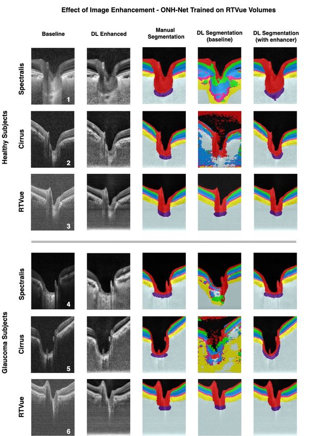
of DL networks. The first (referred to as the enhancer) was able to enhance OCT image quality from
     3 OCT devices, and harmonized image-characteristics across these devices. The second performed 3D
     segmentation of 6 important ONH tissue layers. We found that the use of the enhancer was critical for
     our segmentation network to achieve device independency. In other words, our 3D segmentation network
     trained on any of 3 devices successfully segmented ONH tissue layers from the other two devices with
     high performance (Dice coefficients > 0.92). With such an approach, we could automatically segment
     images from new OCT devices without ever needing manual segmentation data from such devices.

1    Introduction
The complex 3D structural changes of the optic nerve head (ONH) tissues that manifest with the progres-
sion of glaucoma has been extensively studied and better understood owing to the advancements in optical
coherence tomography (OCT) imaging [78]. These include changes such as the thinning of the retinal nerve
fiber layer (RNFL) [10, 62], changes in the choroidal thickness [51], minimum rim width [33], and lamina
curvature and depth [34, 68]. The automated segmentation and analysis of these parameters in 3D from
OCT volumes could improve the current clinical management of glaucoma.

    Robustly segmenting OCT volumes remains extremely challenging. While commercial OCTs have in-
built proprietary segmentation software, they can segment some, but not all the ONH tissues [3, 14, 57].
To address this, several research groups have developed an overwhelming number of traditional image pro-
cessing based 2D [2, 4, 60, 65, 84, 93] and 3D [37, 40, 43, 46, 83, 87] segmentation tools, they are generally
tissue-specific [2, 60, 65, 93, 37, 87], computationally expensive [83, 5], require manual input [40, 46], and
are often prone to errors in scans with pathology [83, 6, 15].

    Recent deep learning (DL) based systems have however exploited a combination of low- (i.e. edge-
information, contrast and intensity profile) and high-level features (i.e. speckle pattern, texture, noise) from
OCT volumes to identify different tissues, yielding human-level [21, 22, 27, 54, 77, 82, 69, 86] and pathology
invariant [21, 22, 69] segmentations. Yet, given the variability in image characteristics (e.g. contrast or
speckle noise) across devices as a result of proprietary processing software [12], a DL system designed for
one device cannot be directly translated to others [79]. Since it is common for clinics to own different OCT
devices, and for patients to be imaged by different OCT devices during their care, the device-specific nature
of these DL algorithms considerably limit their clinical adoption.

    While there currently exists only a few major commercial manufacturers of spectral-domain OCT (SD-
OCT) such as Carl Zeiss Meditec (Dublin, CA, USA), Heidelberg Engineering (Heidelberg, Germany),
Optovue Inc. (Fremont, CA, USA), Nidek (Aichi, Japan), Optopol Technology (Zawiercie, Poland), Canon
Inc. (Tokyo, Japan), Lecia Microsystems (Wetzlar, Germany), etc., several others have already started to or
will soon be releasing the next-generation OCT devices. This further increases the complexity in deploying
DL algorithms clinically. Given that reliable segmentations [12] are an important step towards diagnosing
glaucoma accurately, there is a need for a single DL segmentation framework that is not only translatable
across devices, but also versatile to accept data from next-generation OCT devices.

    In this study, we developed a DL-based 3D segmentation framework that is easily translatable across
OCT devices in a label-free manner (without the need to manually re-segment data for each device). To
achieve this, we first designed an enhancer: a DL network that can improve the quality of OCT B-scans and
harmonize image characteristics across OCT devices. Because of such pre-processing, we demonstrate that
a segmentation framework trained on one device can be used to segment volumes from other unseen devices.

                                                       2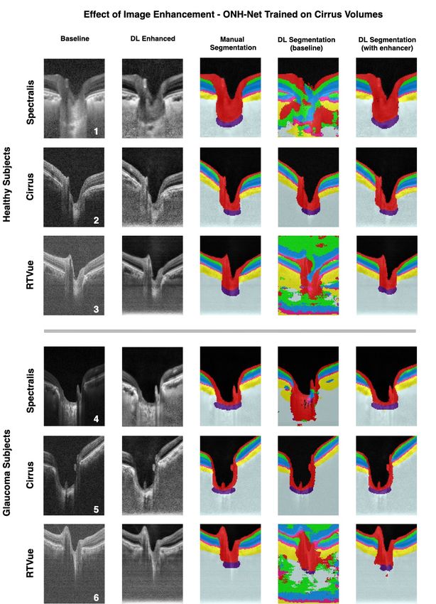
2     Methods
2.1    Overview
The proposed study consisted of two parts: (1) image enhancement, and (2) 3D segmentation.

    We first designed and validated a DL based image enhancement network to simultaneously de-noise (re-
duce speckle noise), compensate (improve tissue visibility and eliminate artefacts) [32], contrast enhance
(better differentiate tissue boundaries) [32], and histogram equalize (reduce intensity inhomogeneity) OCT
B-scans from three commercially available SD-OCT devices (Spectralis, Cirrus, RTVue). The network was
trained and tested with images from all three devices.

   A 3D DL-based segmentation framework was then designed and validated to isolate six ONH tissues from
OCT volumes. The framework was trained and tested separately on OCT volumes from each of the three
devices with and without image enhancement.

2.2    Patient Recruitment
A total of 450 patients were recruited from four centers: the Singapore National Eye Center (Singapore),
Rajan Eye Care Hospital (Chennai, India), Aravind Eye Hospital (Madurai, India), and the East Avenue
Medical Center (Quezon City , Philippines) Table 1. All subjects gave written informed consent. The study
adhered to the tenets of the Declaration of Helsinki and was approved by the institutional review board of
the respective hospitals. The cohort comprised of 225 healthy and 225 glaucoma subjects. The inclusion
criteria for healthy subjects were: an intraocular pressure (IOP) less than 21 mmHg, healthy optic discs with
a vertical cup-disc ratio (VCDR) less than or equal to 0.5, and normal visual fields tests. Glaucoma was
diagnosed with the presence of glaucomatous optic neuropathy (GON), VCDR > 0.7 and/or neuroretinal
rim narrowing with repeatable glaucomatous visual field defects. We excluded subjects with corneal abnor-
malities that could preclude the quality of the scans.

2.3    Optical Coherence Tomography Imaging
All 450 subjects were seated and imaged using spectral-domain OCT under dark room conditions in the re-
spective hospitals. 150 subjects (75 healthy + 75 glaucoma) had one of their ONHs imaged using Spectralis
(Heidelberg Engineering, Heidelberg, Germany), 150 (75 healthy + 75 glaucoma) using Cirrus (model: HD
5000, Carl Zeiss Meditec, Dublin, CA, USA), and another 150 (75 healthy + 75 glaucoma) using RTVue
(Optovue Inc., Fermont, CA, USA). For glaucoma subjects, the eye with GON was imaged, and if both eyes
met the inclusion criteria, one eye was randomly selected. For healthy controls, the right ONH was imaged.
The scanning specifications for each device can be found in Table 1.

   From the dataset of 450 volumes, 390 (130 from each device) were used for training and testing the image
enhancement network, while the remaining 60 (20 from each device) were used for training and testing the
3D segmentation framework.

2.4    Image Enhancement
The enhancer network was trained to reproduce simple mathematical operations including spatial averaging,
compensation, contrast enhancement, and histogram equalization. When using images from a single device,
the use of a DL network to perform such operations would be seen as unnecessary, as one could readily use
the mathematical operators instead. However, when mixing images from multiple devices, besides perform-
ing such enhancement operations, the network also reduces the differences in the image characteristics across
the devices, resulting in images that are harmonized (i.e. less device specific) a necessary step to perform

                                                     3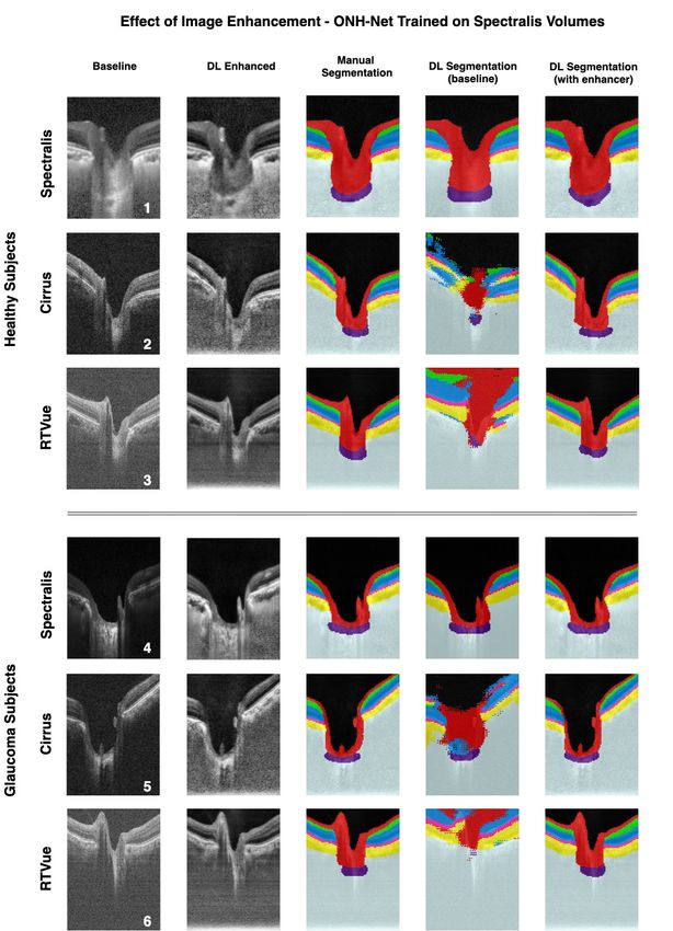
No of subjects
   Device                Hospital                                              Scanning Specifications
                                               Normal Glaucoma
                                                                       97 horizontal B-scans
              Singapore National Eye Center    57           11         32 µm distance between B-scans
 Spectralis                                                            area of 15 ◦ x 10 ◦
              Aravind Eye Hospital             18           64         centered on the ONH
                                                                       20x signal averaging.
                                                                       200 horizontal B-scans
   Cirrus     Rajan Eye Care Hospital          75           75         30 µm, 200 A-scans per B-scans
                                                                       area of 6mm x 6mm centered on the ONH
                                                                       101 horizontal B-scans
                                                                       40 µm distance between B-scans
  RTVue       East Avenue Medical Center       75           75
                                                                       101 A-scans per B-scan
                                                                       area of 20 ◦ x 20 ◦ centered on the ONH

       Table 1: A summary of patient populations and scanning specifications for each OCT device.

robust device-independent 3D segmentation.

2.5    Image Enhancement Dataset Preparation
The 390 volumes were first resized (in pixels) to 448 (height) x 352 (width) x 96 (number of B-scans), and
a total of 37,440 baseline B-scans (12,480 per device) were obtained. Each B-scan (Figure 1 A[1]) was
then digitally enhanced (Figure 1 A[4]) by performing spatial averaging (each pixel value was replaced by
the mean of its 8 lateral neighbors; Figure 1 A[2]) [89], compensation and contrast enhancement (contrast
exponent = 2; Figure 1 A[3]) [32], and histogram equalization (contrast limited adaptive histogram equal-
ization [CLAHE], clip limit = 2; Figure 1 A[4]) [71].

    The image enhancement network was then trained with 36,000 pairs (12,000 per device) of baseline and
digitally-enhanced B-scans, respectively. Another 1,440 pairs were used for testing. B-scans from a same
patient were not shared between training and testing.

2.6    Image Enhancement Network Description
Briefly, as in our earlier DL based image enhancement study [23], the proposed enhancer exploited the in-
herent advantages of U-Net38 and its skip connections [61], residual learning [44], dilated convolutions [92],
and multi-scale hierarchical feature extraction [53]. We used the same network architecture, except that
the output layer was now activated by the sigmoid activation function [67] (originally tanh). The design,
implementation, significance of each component, and data augmentation details can be referred to from our
earlier study [23]. The loss function was a weighted combination of both the root mean square error (RMSE)
and a multi-scale perceptual loss [41] function that was based on the VGG19 DL model [80].

    Pixel-to-pixel loss functions (e.g., RMSE) compare only the low-level features (i.e., edge information)
between the DL prediction and their corresponding ground-truth often leading to over-smoothened (blur)
images [41], especially in image-to-image translation problems (e.g., de-noising). However, perceptual loss
based functions exploit the high-level features (i.e., texture, abstract patterns) [41, 13, 7, 50] in these images
to assess their differences, enabling the DL network to achieve human-like visual understanding [94]. Thus,
a weighted combination of both the loss functions allows the DL network to preserve the low- and high- level
features in its predictions, limiting the effects of blurring.

                                                        4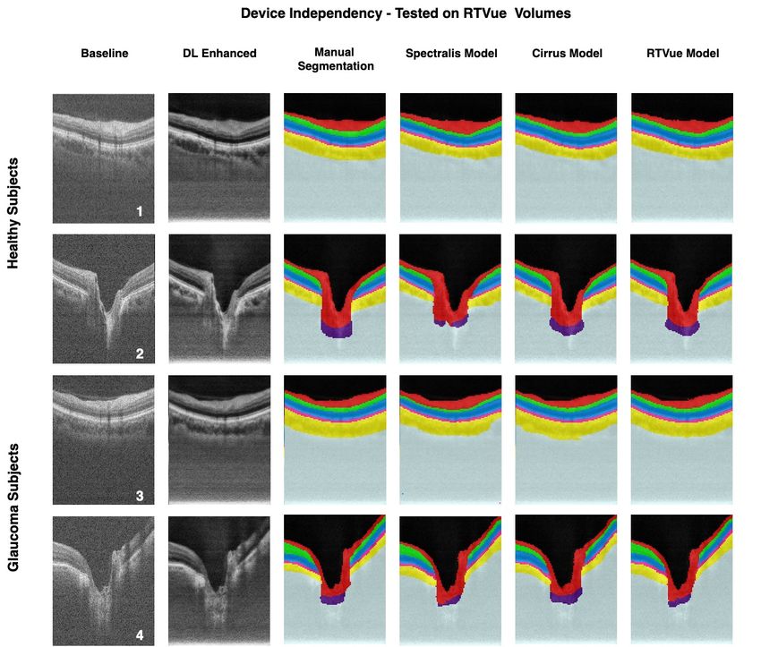
Figure 1: The dataset preparation for the image enhancement network is shown in (A). Each B-scan (A [1])
was digitally enhanced (4) by performing spatial averaging (each pixel value was replaced by the mean of
its 8 lateral neighbors; A [2]), compensation and contrast enhancement (contrast exponent = 2; A[3]), and
histogram equalization (contrast limited adaptive histogram equalization [CLAHE], clip limit = 2; A[4]).
For training the 3D segmentation framework (B), the following tissues were manually segmented from OCT
volumes: (1) the RNFL and prelamina (in red), (2) the ganglion cell complex (GCC; ganglion cell layer
+ inner plexiform layer; in cyan), (3) all other retinal layers (in blue); (4) the retinal pigment epithelium
(RPE; in pink); (5) the choroid (in yellow); and (6) the lamina cribrosa (LC; in indigo). Noise (in grey) and
vitreous humor (in black) were also isolated.

                                                     5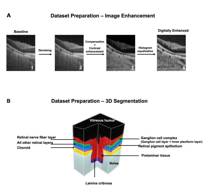
To compute the perceptual loss, the output of the enhancer (referred to as ’DL-enhanced’ B-scan) and
its corresponding digitally-enhanced B-scan was separately passed through the VGG-19 [80] DL model that
was pre-trained on the ImageNet dataset [19]. Feature maps at multiple scales (outputs from the 2nd, 4th,
6th, 10th, and 14th convolutional layers) were extracted, and the perceptual loss was computed as the mean
RMSE (average of all scales) between the extracted features from the DL-enhanced and its corresponding
digitally-enhanced B-scan.

   Experimentally, the RMSE and perceptual loss when combined in a weighted-ratio of 1.0:0.01 offered the
best performance (qualitative and quantitative; as described below).

    The enhancer comprised of a total of 900 K trainable parameters, and was trained end-to-end using
the Adam optimizer [24], with a learning rate of 0.0001. We trained and tested on an NVIDIA GTX 1080
founders edition GPU with CUDA 10.1 and cuDNN v7.5 acceleration. Using the given hardware configura-
tion, the DL network enhanced a single baseline B-scan in under 25 ms.

2.7    Image Enhancement Qualitative Analysis
Upon training, the network was used to enhance the unseen baseline B-scans from all the three devices.
The DL-enhanced B-scans were qualitatively assessed by two expert observers (S.K.D and T.P.H) for the
following: (1) noise reduction, (2) deep tissue visibility and blood vessel shadows, (3) contrast enhancement
and intensity inhomogeneity, and (4) DL induced artifacts.

2.8    Image Enhancement Quantitative Analysis
The following metrics were used to quantitatively assess the performance of the enhancer: (1) universal
image quality index (UIQI) [96], and (2) structural similarity index (SSIM) [97]. We used the UIQI to assess
the extent of image enhancement (baseline vs. DL-enhanced B-scans), while the MSSIM was used to assess
the structural reliability of the DL-enhanced B-scans (digitally-enhanced vs. DL-enhanced).

    Unlike the traditional error summation methods (e.g., RMSE etc.) that compared only the intensity dif-
ferences, the UIQI jointly modeled the (1) loss of correlation (LC ), (2) luminance distortion (DL ), and (3)
contrast distortion (DC ) to assess image quality [96]. It was defined as (x: baseline; y: DL-enhanced B-scan):

                                        U IQI(x, y) = LC × DL × DC

   where,

                                         σxy         2µx µy         2σx σy
                                 LC =         ; DL = 2     2
                                                             ; DC = 2
                                        σx σy       µx + µy        σx + σy2

   (LC ) measured the degree of linear correlation between the baseline and DL-enhanced B-scans; (DL ) and
(DC ) measured the distortion in luminance and contrast respectively; µx , σx , σx2 denoted the mean, standard
deviation, and variance of the intensity for B-scan x, while µy , σy , σy2 denoted the same for the B-scan y; σxy
was the cross-covariance between the two B-scans. The UIQI was defined between -1 (poor quality) and +1
(excellent quality). As in our previous study [23], the SSIM (x: digitally-enhanced; y: DL-enhanced B-scan)
was defined as:

                                                       6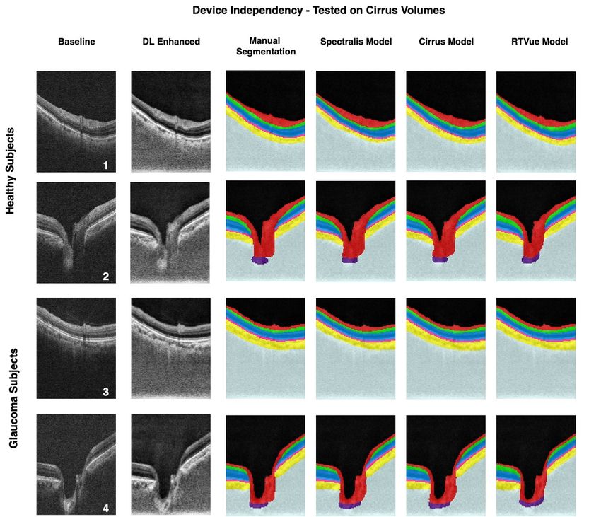
(2µx µy + C1 )(2σxy + C2 )
                               SSIM (x, y) =
                                               (µ2x + µ2y + C1 )(σx2 + σy2 + C2 )

   The constants C1 and C2 (to stabilize the division) were chosen as 6.50 and 58.52, as recommended in a
previous study [97]. The SSIM was defined between -1 (no similarity) and +1 (perfect similarity).

2.9    3D Segmentation Dataset Preparation
The 60 volumes used for training and testing the 3D segmentation framework (20 from each device, balanced
with respect to pathology) were manually segmented (slice-wise) by an expert observer (SD) using Amira
(version 6, FEI, Hillsboro, OR). The following classes of tissues were segmented (Figure 1 B): (1) the RNFL
and prelamina (in red), (2) the ganglion cell complex (GCC; ganglion cell layer + inner plexiform layer;
in cyan), (3) all other retinal layers (in blue); (4) the retinal pigment epithelium (RPE; in pink); (5) the
choroid (in yellow); and (6) the lamina cribrosa (LC; in indigo). Noise (all regions below the choroid-sclera
interface; in grey) and vitreous humor (black) were also isolated. We were unable to obtain a full-thickness
segmentation of the LC due to limited visibility [59]. We also excluded the peripapillary sclera due to its
poor visibility and the extreme subjectivity of its boundaries especially in Cirrus and RTVue volumes. To
optimize computational speed, the volumes (baseline OCT + labels) for all three devices were resized (in
voxels) to 112 (height) x 88 (width) x 48 (number of B-scans).

2.10    Deep Learning Based 3D Segmentation of the ONH
Recent studies have demonstrated that 3D CNNs can improve the reliability of automated segmentation
[63, 20, 98, 76, 38, 64, 75, 25], and even out-perform their 2D variants [20]. This is because 3D CNNs not
only harness the information from each image, but also effectively combine it with the depth-wise spatial
information from adjacent images. Despite its tremendous potential, the applications of 3D CNNs in oph-
thalmology is still in its infancy [1, 28, 26, 49, 66, 56], and has not yet been explored for the segmentation
of the ONH tissues.

    Further, there exist discrepancies in the delineation of ambiguous regions (e.g., choroid-sclera boundary,
LC boundary) even among different well-trained DL model depending upon the type and complexity of
architecture/feature extraction, learning method, etc., causing variability in the automated measurements.
To address this, recent DL studies have explored ensemble learning [69, 8, 18, 31, 45, 52, 55, 73, 95, 48], a
meta-learning approach that synergizes (combine and fine-tune) [55] the predictions from multiple networks,
to offer a single prediction that is closest to the ground-truth. Specifically, ensemble learning has shown to
better generalize and increase the robustness of segmentations in OCT [69, 18] and other medical imaging
modalities [31, 45, 52, 95].

    In this study, we designed and validated ONH-Net, a 3D segmentation framework inspired by the popular
3D U-Net [98] to isolate six ONH tissues from OCT volumes. The ONH-Net consisted of three segmentation
networks (3D CNNs) and one 3D CNN for ensemble learning (referred to as the ensembler). Each of the three
segmentation CNNs offered an equally plausible segmentation, which were then synergized by the ensembler
to yield the final 3D segmentation of the ONH tissues.

2.11    3D Segmentation Network Description
The design of the three segmentation CNNs was based on the 3D U-Net [98] and its variants [28]. Each of
the three segmentation CNNs (Figure 2 A) comprised of four micro-U-Nets (µ-U-Nets; Figure 2 B), and
a latent space (Figure 2 C).Both the segmentation CNNs and the µ-U-Nets followed a similar design style.

                                                      7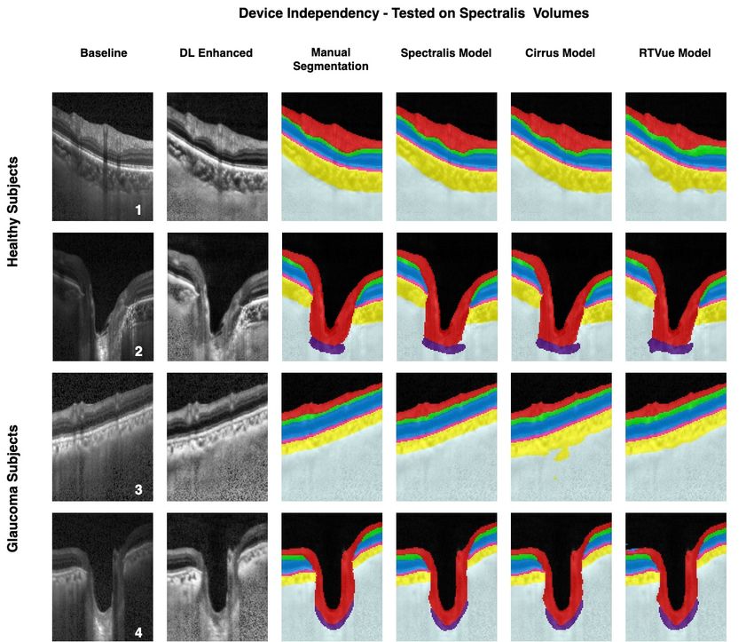
They consisted of an encoder segment that extracted contextual features (i.e. spatial arrangement of
tissues), and a decoder segment that extracted the local information (i.e. tissue texture). The encoder seg-
ment sequentially downsampled the feature maps using the 3D max-pooling layers (stride=2,2,2), while the
decoder segment sequentially upsampled using the 3D transposed convolutional layers (stride=2,2,2; filter
size: 3x3x3; no of filters: 48).

   The latent space, implemented using residual blocks similar to our earlier study [23], transferred the ex-
tracted features from the encoder to the decoder segment. The use of residual learning improved the flow of
gradient information through the network. Skip connections [74] between the encoder and decoder segments
helped the DL network to jointly learn the contextual and local information, and the relationships between
them.

   Also, as implemented in our earlier study [23], we used multi-scale hierarchical feature extraction to im-
prove the delineation of tissue boundaries. The feature maps obtained from multi-scale hierarchical feature
extraction were then added with the output of the decoder segment.

   The three segmentation CNNs deferred from each other only in the design of the ’feature extraction’
(FE) units (Figure 2 D; Types 1-3) that were used in the µ-U-Nets.

   The Type 1 and Type 2 FE (Figure 2 D; Types 1-2) units had a similar design, except that the input
was pre-activated by the elu activation [16] in Type 2 FE.

    In both the FE units, the input was passed through three parallel pathways: (1) the identity pathway;
(2) the planar pathway; and (3) the volumetric pathway. The identity pathway implemented using a 1x1x1
3D convolutional layer allowed the unimpeded flow of gradient information throughout the network. In the
planar pathway, the information from any two dimensions was extracted by the network at once (filter size:
3x3x1 [height x width]; 3x1x3 [height x depth]; 1x3x3 [width x depth]; 48 filters each). The volumetric
pathway exploited the depth-wise spatially related and continuous information from all three dimensions at
once (i.e., tissue morphology) using three 3D convolutional layers (filter size: 3x3x3; no of filters: 48).Fi-
nally, the feature maps from all the three pathways were added, batch normalized [39], and elu activated [16].

     In the Type 3 FE (Figure 2 D) unit, the input was elu activated and passed on to three sets of simple
residual blocks with 48, 96, and 144 filters, respectively. In each residual block, one 3D convolutional layer
(filter size: 3x3x3) extracted the features, while a 1x1x1 3D convolution layer was used as the identity con-
nection [44]. The feature maps were then added, elu activated, and passed on to the next block. Finally, the
feature maps were batch normalized and elu activated.

    For all three segmentation CNNs, the pre-final output feature maps (decoder output + multi-scale hi-
erarchical feature extraction) were passed through a 3D convolutional layer (filter size: 1x1x1; no of filters:
8 [number of classes; 6 tissues + noise + vitreous humor]) and softmax activated to obtain the tissue-wise
probability for each pixel. For each pixel, the tissue class of the highest probability was then assigned.

    The ensembler (Figure 2 E) was then implemented using three sets of 3D convolutional layers (specifi-
cations for each set; filter size [no of filters]: 3x3x3 [48]; 3x3x3 [96]; 3x3x3 [192]). A dropout [81] of 0.50 was
used between each set to reduce overfitting and improve the generalizability of the DL network. The feature
maps were then passed through two dense layers of 64 and 8 units (number of classes) respectively, that
were separated by a dropout layer (0.50). Finally, a softmax activation was applied to obtain the pixel-wise
predictions.

  Each of the three segmentation CNNs were first trained end-to-end with the same labeled-dataset. The
ONH-Net was then assembled by using the three trained CNNs as parallel input pipelines to the ensem-

                                                        8
bler network (Figure 2 F). Finally, we trained the ONH-Net (ensembler weights: trainable; segmentation
CNN weights: frozen) end-to-end using the same aforementioned labeled-dataset. During this process, each
segmentation CNN provided equally plausible segmentation feature maps (obtained from the last 3D con-
volution layer), which were then concatenated and fed to the ensembler for fine-tuning. The ONH-Net was
trained separately for each device.
All the DL networks (segmentation CNNs, ONH-Net) were trained with the stochastic gradient descent
(SGD; learning rate:0.01; Nestrov momentum:0.05 [85]) optimizer, and the Jaccard distance was used as the
loss function [22]. We empirically observed that the use of SGD optimizer with Nesterov momentum offered
a better generalizability and faster convergence compared to Adam optimizer [24] for OCT segmentation
problems that typically use limited data, while Adam performed better for image-to-image translation prob-
lems (i.e., enhancement [23]) that use much larger datasets. However, we are unable to theoretically explain
this yet for our case. Given the limitations in hardware, all the DL networks were trained with a batch size
of 1. To circumvent the scarcity in data, all the DL networks used custom data augmentation techniques
(B-scans wise) as in our earlier study [22]. We ensured that the same data augmentation was used for each
B-scan in a given volume.
The three CNNs consisted of 7.2 M (Type 1), 7.2 M (Type 2), and 12.4 M (Type 3) trainable parameters,
while the ONH-Net consisted of 28.86 M parameters (2.06M trainable parameters [ensembler], 26.8M non-
trainable parameters [trained CNNs with weights frozen]). All the DL networks were trained and tested on
NVIDIA GTX 1080 founders edition GPU with CUDA 10.1 and cuDNN v7.5 acceleration. Using the given
hardware configuration, the ONH-Net was trained in 12 hours (10 hours for each CNN [trained in parallel;
one per GPU]; 2 hours for fine-tuning with the ensembler). Once trained, each OCT volume was segmented
in about 120 ms.
2.12 3D Segmentation Training and Testing
We used a five-fold cross-validation approach (for each device) to train and test the performance of ONH-
Net. In this process, the labeled-dataset (20 OCT volumes + manual segmentations) was split into five equal
parts. One part (left-out set; 4 OCT volumes + manual segmentations) was used as the testing dataset,
while the remaining four parts (16 OCT volumes + manual segmentations) were used as the training dataset.
The entire process was repeated five times, each with a different left-out testing dataset (and corresponding
training dataset). Totally, for each device, the segmentation performance was assessed on 20 OCT volumes
(4 per validation; 5-fold cross-validation).
2.13 3D Segmentation Performance Qualitative Analysis
The segmentations obtained from the trained ONH-Net on unseen data were manually reviewed by expert
observers (S.D. and T.P.H) and compared against their corresponding manual segmentations.
2.14 3D Segmentation Performance Quantitative Analysis
We used the following metrics to quantitatively assess the segmentation performance: (1) Dice coefficient
(DC); (2) specificity (Sp); and (3) sensitivity (Sn). The metrics were computed in 3D for the following
tissues: (1) the RNFL and prelamina; (2) the GCC; (3) all other retinal layers; (4) the RPE; and (5)
the choroid. Given the subjectivity in the visibility of the posterior LC boundary [59], we excluded LC
from quantitative assessment. Noise and vitreous humor were also excluded from quantitative assessment.
The Dice coefficient (DC) was used to assess the spatial overlap between the manual and DL segmentations
(between 0 [no overlap] and 1 [perfect overlap]). For each tissue, the DC was computed as:
92 × |D ∩ M |
Dice score (DC) =
2 × |D ∩ M | + |D \ M | + |M \ D|
where D and M were the voxels that represented the chosen tissue in the DL segmented and the cor-
responding manually segmented volumes. Specificity (Sp) was used to assess the true negative rate of the
segmentation framework, while sensitivity (Sn) was used to assess the true positive rate. They were defined
as:
|D ∩ M | |D ∩ M |
Specificity (Sp) = ; Sensitivity =
|M | |M |
where D represented the voxels that did not belong to the chosen tissue in the DL segmented volume,
while M represented the same in the corresponding manually segmented volume.
2.15 3D Segmentation Performance Effect of Image Enhancement
To assess if image enhancement had an effect on segmentation performance, we trained and tested ONH-Net
on the baseline and the DL-enhanced datasets. For both datasets, ONH-Net was trained on any one device
(Spectralis/Cirrus/RTVue), but tested on all the three devices (Spectralis, Cirrus, and RTVue). Paired
t-tests were used to compare the differences (means) in the segmentation performance (Dice coefficients,
sensitivities, specificities; mean of all tissues) for both cases.
2.16 3D Segmentation Performance Device Independency
When tested on a given device (Spectralis/Cirrus/RTVue), paired t-tests were used to assess the differences
(Spectralis vs. Cirrus; Cirrus vs. RTVue; RTVue vs. Spectralis) in the segmentation performance depending
on the device used for training ONH-Net. The process was performed with both baseline and DL-enhanced
datasets.
2.17 3D Segmentation Clinical Reliability Automated Parameter Extraction
Upon obtaining the DL segmentations, two clinically relevant structural parameters that are crucial for the
diagnosis of glaucoma: the (1) peripapillary RNFL thickness (p-RNFLT); and the (2) peripapillary GCC
thickness (p-GCCT) were automatically extracted as in our earlier works.
For each volume in the testing dataset, a circular scan of diameter 3.4mm centered around the ONH
[30] was obtained. The p-RNFL thickness (global) was computed as the distance between the inner limiting
membrane and the posterior RNFL boundary (mean of 360◦ measure). The p-GCT (global) was computed
as the distance between the posterior RNFL boundary and the inner plexiform layer boundary (mean of
360◦ measure).
The intraclass correlation coefficients (ICCs) were obtained to compare the measurements computed from
the DL and their corresponding manual segmentations for all cases.
10Figure 2: The DL architecture of the proposed 3D segmentation framework (three segmentation CNNs +
one ensembler network) is shown. Each CNN (A) comprised of four micro-U-Nets (µ-U-Nets; (B)) and a
latent space (LS; (C)). The three CNNs differed from each other only in the design of the ’feature extraction’
(FE) units ((D); Types 1-3). The ensembler (E) consisted of three sets of 3D convolutional layers, with
each set separated by a dropout layer. ONH-Net (F) was then assembled by using the three trained CNNs
as parallel input pipelines to the ensembler network.
113 Results
3.1 Image Enhancement Qualitative Analysis
The enhancer was tested on a total of 1440 (480 from each device) unseen baseline B-scans. In the DL-
enhanced B-scans from all the three devices (Figure 3, Column 3), the ONH-tissue boundaries appeared
sharper with an uniformly enhanced intensity profile (compared to respective baseline B-scans). The blood
vessel shadows were also reduced with improved deep tissue (choroid-scleral interface, LC) visibility. In all
cases, the DL-enhanced B-scans were consistently similar to their corresponding digitally-enhanced B-scans
(Figure 3, Column 2), with no DL induced artifacts.
3.2 Image Enhancement Quantitative Analysis
The mean UIQI (mean ± SD) for the DL-enhanced B-scans (compared to baseline B-scans) were: 0.94 ±
0.02, 0.95 ± 0.03, and 0.97 ± 0.01 for Spectralis, Cirrus, and RTVue, respectively, indicating improved image
quality.
In all cases, the mean SSIM (mean ± SD) for the DL-enhanced B-scans (compared to digitally-enhanced
B-scans) were: 0.95 ± 0.02, 0.91 ± 0.02, and 0.93 ± 0.03, for Spectralis, Cirrus, and RTVue, respectively,
indicating strong structural similarity.
3.3 3D Segmentation Performance Qualitative Analysis
When trained and tested on the baseline volumes from the same device (Figure 4 - Figure 6; 4th
column), ONH-Net successfully isolated all ONH layers. Further, the DL segmentations appeared consistent
with their respective manual segmentations (Figure 4 - Figure 6; 3rd column), with no difference in
the segmentation performance between glaucoma and healthy OCT volumes. A representative case of the
segmentations in 3D when trained on Spectralis and tested on the other three devices is shown in Figure 7.
3.4 3D Segmentation Performance Quantitative Analysis
When trained and tested on the baseline volumes (same device), the mean Dice coefficients (mean of all
tissues; mean ± SD) were: 0.93 ± 0.02, 0.93 ± 0.02, and 0.93 ± 0.02 for Spectralis, Cirrus, and RTVue,
respectively. The mean sensitivities / specificities (mean of all tissues; mean SD) were: 0.94 ± 0.02 / 0.99
± 0.00, 0.93 ± 0.02 / 0.99 ± 0.00, and 0.93 ± 0.02 / 0.99 ± 0.00, respectively.
3.5 3D Segmentation Performance Effect of Image Enhancement and Device
Independency
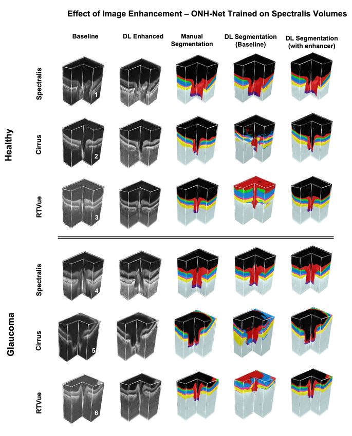
Without image enhancement (baseline dataset), ONH-Net trained with one device was unable to segment
even a single ONH tissue reliably on the other two devices (Figure 4 ; Rows 2,3,5,6; Column 4; similarly
for Figures 5 - 6). In all cases, dice coefficients were always lower than 0.65, sensitivities lower than 0.77,
and specificities lower than 0.80.
However, with image enhancement (DL-enhanced dataset), ONH-Net trained with one device was able
to accurately segment all tissue layers on the other two devices with mean Dice coefficients and sensitivities
> 0.92 (Figures 4-6, Column 5). In addition, when trained and tested on the same device, it performed
better for several ONH layers (p < 0.05), when it was tested on the same device that it was trained on. The
tissue wise quantitative metrics for the aforementioned cases can be found in Tables 2-4.
Further, when trained and tested with the DL-enhanced OCT volumes, irrespective of the device used
for training, there were no significant differences (p(Figures 8-10), except for the LC. The tissue wise quantitative metrics for the individual cases can be
found in Tables 5-7.
3.6 3D Segmentation Clinical Reliability Automated Parameter Extraction
When trained and tested (same device) on the baseline OCT volumes, the ICCs were always greater than
0.99 for both the p-RNFLT and the p-GCCT. However, when tested on the other two devices, since that
the ONH-Net was unable to segment even a single tissue reliably, we did not extract the p-RNFLT and the
g-GCCT for these cases.
When repeated the same with the DL-enhanced volumes, irrespective of the device used for training, the
ICCs were always greater than 0.98 for all cases, indicating excellent reliability.
Effect of Image Enhancement - Spectralis Trained Framework
RNFL GCC Other Retinal Layers RPE Choroid
Testing Device
w/o w w/o w w/o w w/o w w/o w
DC 0.9510.023 0.9540.017 0.8980.0216 0.9310.020 0.9120.011 0.9360.010 0.8960.010 0.9180.014 0.9020.044 0.926 0.031
Spectralis Sn 0.9460.031 0.9600.026 0.9000.0290 0.9460.019 0.9170.009 0.9470.010 0.9060.025 0.9380.022 0.9150.054 0.931 0.038
Sp 0.9970.005 0.9930.001 0.9950.002 0.9960.003 0.9950.000 0.9950.001 0.9940.001 0.9940.002 0.9950.004 0.996 0.002
DC 0.5110.029 0.9430.027 0.3020.061 0.9190.032 0.5870.035 0.9180.031 0.5620.020 0.9180.019 0.4770.055 0.902 0.033
Cirrus Sn 0.7010.035 0.9550.024 0.5600.0312 0.8990.024 0.7370.022 0.9370.020 0.6830.019 0.9200.023 0.6870.057 0.896 0.043
Sp 0.7810.004 0.9880.000 0.7020.005 0.9830.004 0.8110.001 0.9920.004 0.7970.002 0.9910.001 0.7970.005 0.991 0.004
DC 0.3230.048 0.9510.031 0.2810.068 0.8980.030 0.2880.060 0.8960.041 0.3370.055 0.9120.029 0.3570.059 0.934 0.028
RTVue Sn 0.5170.039 0.9360.032 0.4650.063 0.9310.038 0.4660.051 0.9130.038 0.5250.043 0.9100.031 0.5130.061 0.901 0.028
Sp 0.6780.006 0.9960.003 0.5220.009 0.9920.006 0.5980.005 0.9940.005 0.7280.006 0.9940.003 0.7100.010 0.994 0.005
Table 2: The quantitative segmentation performance (DC: Dice coefficient; Sn: sensitivity; Sp: speci-
ficity) of ONH-Net with (w) and without (w/o) the use of image enhancement. ONH-Net was trained
on Spectralis, and tested on Spectralis, Cirrus, RTVue devices. The metrics for each tissue that were
significantly higher (pEffect of Image Enhancement - Cirrus Trained Framework
RNFL GCC Other Retinal Layers RPE Choroid
Testing Device
w/o w w/o w w/o w w/o w w/o w
DC 0.7440.033 0.9660.027 0.6940.045 0.9350.020 0.6990.039 0.9230.023 0.6070.038 0.9320.018 0.5420.041 0.937 0.029
Spectralis Sn 0.7410.037 0.9460.031 0.7900.028 0.9340.021 0.8140.033 0.9490.027 0.7500.040 0.9320.032 0.7730.048 0.940 0.034
Sp 0.7850.004 0.9870.000 0.7670.003 0.9920.002 0.8580.003 0.9940.002 0.8010.003 0.9950.003 0.8470.005 0.995 0.002
DC 0.9120.023 0.9650.022 0.8300.034 0.9200.027 0.8990.029 0.9320.026 0.8630.032 0.9130.020 0.8670.039 0.924 0.025
Cirrus Sn 0.9360.031 0.9740.030 0.8990.028 0.9180.026 0.9000.020 0.9220.021 0.9070.026 0.9330.015 0.9130.033 0.923 0.028
Sp 0.9710.002 0.9880.001 0.9840.002 0.9940.002 0.9910.004 0.9950.001 0.9910.002 0.9960.002 0.9890.001 0.993 0.005
DC 0.6430.051 0.9360.035 0.5410.055 0.8960.029 0.5380.059 0.9170.028 0.6450.060 0.9050.030 0.4930.064 0.910 0.031
RTVue Sn 0.6430.048 0.9250.033 0.6420.059 0.9200.031 0.6600.048 0.9280.022 0.7250.051 0.9250.027 0.7650.055 0.926 0.034
Sp 0.7000.010 0.9800.003 0.6680.010 0.9860.004 0.7080.004 0.9880.003 0.7810.005 0.9900.004 0.8060.009 0.990 0.005
Table 3: The quantitative segmentation performance (DC: Dice coefficient; Sn: sensitivity; Sp: speci-
ficity) of ONH-Net with (w) and without (w/o) the use of image enhancement. ONH-Net was trained
on Cirrus, and tested on Spectralis, Cirrus, RTVue devices. The metrics for each tissue that were
significantly higher (pFigure 3: The qualitative performance of the image enhancement network is shown for six randomly selected
(1-6) subjects (2 per device). The 1st, 2nd and 3rd columns represent the baseline, digitally-enhanced, and
the corresponding DL-enhanced B-scans for patients imaged with Spectralis (1-2), Cirrus (3-4), and RTVue
(5-6) devices, respectively.
15Figure 4: The qualitative performance (one randomly chosen B-scan per volume) of the ONH-Net 3D seg-
mentation framework for three healthy (1-3) and three glaucoma (4-6) subjects is shown. The framework
was trained on volumes from Spectralis, and tested on Spectralis (1,4), Cirrus (2,5), and RTVue (3,6) de-
vices respectively. The 1st, 2nd and 3rd columns represent the baseline, DL enhanced, and the corresponding
manual segmentation for the chosen B-scan. The 4th and 5th columns represent the DL segmentations when
ONH-Net was trained and tested using the baseline and DL enhanced volumes, respectively.
16Figure 5: The qualitative performance (one randomly chosen B-scan per volume) of the ONH-Net 3D
segmentation framework for three healthy (1-3) and three glaucoma (4-6) subjects is shown. The framework
was trained on volumes from Cirrus, and tested on Spectralis (1,4), Cirrus (2,5), and RTVue (3,6) devices
respectively. The 1st, 2nd and 3rd columns represent the baseline, DL enhanced, and the corresponding
manual segmentation for the chosen B-scan. The 4th and 5th columns represent the DL segmentations when
ONH-Net was trained and tested using the baseline and DL enhanced volumes, respectively.
17Figure 6: The qualitative performance (one randomly chosen B-scan per volume) of the ONH-Net 3D
segmentation framework for three healthy (1-3) and three glaucoma (4-6) subjects is shown. The framework
was trained on volumes from RTVue, and tested on Spectralis (1,4), Cirrus (2,5), and RTVue (3,6) devices
respectively. The 1st, 2nd and 3rd columns represent the baseline, DL enhanced, and the corresponding
manual segmentation for the chosen B-scan. The 4th and 5th columns represent the DL segmentations when
ONH-Net was trained and tested using the baseline and DL enhanced volumes, respectively.
18Figure 7: The segmentation performance (in 3D) on three healthy (1-3) and three glaucoma (4-6) subjects is
shown. The ONH-Net was trained on volumes from Spectralis, and tested on Spectralis (1, 4), Cirrus (2, 5),
and RTVue (3,6) devices respectively. The 1,st 2,nd and 3rd columns represent the baseline, DL enhanced,
and the corresponding manual segmentations for the chosen volumes. The 4th and 5th columns represent
the DL segmentations when the ONH-Net was trained with and without image enhancement respectively.
19Figure 8: The device independent segmentation performance of the proposed ONH-Net is shown. The
segmentation performance on four randomly chosen (1-2 healthy; 3-4 glaucoma) Spectralis volumes from
the test set are shown (one B-scan per volume). The 1st, 2nd, and 3rd columns represent the baseline,
DL enhanced and the corresponding manual segmentation for the chosen B-scan. The 4th, 5th, and 6th
columns represent the segmentations obtained when tested using the Spectralis, Cirrus, and RTVue trained
segmentation model.
20Figure 9: The device independent segmentation performance of the proposed ONH-Net is shown. The
segmentation performance on four randomly chosen (1-2 healthy; 3-4 glaucoma) Cirrus volumes from the test
set are shown (one B-scan per volume). The 1st, 2nd, and 3rd columns represent the baseline, DL enhanced
and the corresponding manual segmentation for the chosen B-scan. The 4th, 5th, and 6th columns represent
the segmentations obtained when tested using the Spectralis, Cirrus, and RTVue trained segmentation model.
21Figure 10: The device independent segmentation performance of the proposed ONH-Net is shown. The
segmentation performance on four randomly chosen (1-2 healthy; 3-4 glaucoma) RTVue volumes from
the test set are shown (one B-scan per volume). The 1st, 2nd, and 3rd columns represent the baseline,
DL enhanced and the corresponding manual segmentation for the chosen B-scan. The 4th, 5th, and 6th
columns represent the segmentations obtained when tested using the Spectralis, Cirrus, and RTVue trained
segmentation model.
22Training Device
Tissue (Spectralis Volumes)
Spectralis Cirrus RTVue
DC 0.9540.017 0.9660.027 0.9660.029
RNFL Sn 0.9600.026 0.9460.031 0.9510.035
Sp 0.9930.001 0.9870.000 0.9860.003
DC 0.9310.020 0.9350.020 0.9120.028
GCC Sn 0.9460.019 0.9340.021 0.9150.028
Sp 0.9960.003 0.9920.002 0.9940.003
DC 0.9360.010 0.9230.023 0.9180.026
Other Retinal Layers Sn 0.9470.010 0.9490.027 0.9310.031
Sp 0.9950.001 0.9940.002 0.9960.001
DC 0.9180.014 0.9320.018 0.9150.020
RPE Sn 0.9380.022 0.9320.032 0.9170.036
Sp 0.9940.002 0.9950.003 0.9960.003
DC 0.926 0.031 0.937 0.029 0.915 0.021
Choroid Sn 0.931 0.038 0.940 0.034 0.922 0.033
Sp 0.996 0.002 0.995 0.002 0.985 0.006
Table 5: The device independent segmentation performance (DC: Dice coefficient; Sn: sensitivity; Sp:
specificity) of ONH-Net (using DL-enhanced dataset). The volumes from Spectralis device were tested on
three segmentation models (Spectralis, Cirrus, and RTVue trained).
Training Device
Tissue (Cirrus Volumes)
Spectralis Cirrus RTVue
DC 0.9430.027 0.9650.022 0.9420.024
RNFL Sn 0.9550.024 0.9740.030 0.9540.033
Sp 0.9880.000 0.9880.001 0.9950.002
DC 0.9190.032 0.9200.027 0.9390.024
GCC Sn 0.8990.024 0.9180.026 0.9160.028
Sp 0.9830.004 0.9940.002 0.9930.004
DC 0.9180.031 0.9320.026 0.9070.031
Other Retinal Layers Sn 0.9370.020 0.9220.021 0.9220.030
Sp 0.9920.004 0.9950.001 0.9940.002
DC 0.9180.019 0.9130.020 0.9090.029
RPE Sn 0.9200.023 0.9330.015 0.9010.035
Sp 0.9910.001 0.9960.002 0.9840.008
DC 0.902 0.033 0.924 0.025 0.911 0.027
Choroid Sn 0.896 0.043 0.923 0.028 0.905 0.025
Sp 0.991 0.004 0.993 0.005 0.993 0.002
Table 6: The device independent segmentation performance (DC: Dice coefficient; Sn: sensitivity; Sp:
specificity) of ONH-Net (using DL-enhanced dataset). The volumes from Cirrus device were tested on
three segmentation models (Spectralis, Cirrus, and RTVue trained).
23Training Device
Tissue (RTVue Volumes)
Spectralis Cirrus RTVue
DC 0.9510.031 0.9360.035 0.9510.028
RNFL Sn 0.9360.032 0.9250.033 0.9470.010
Sp 0.9960.003 0.9800.003 0.9970.001
DC 0.8980.030 0.8960.029 0.9110.017
GCC Sn 0.9310.038 0.9200.031 0.9280.019
Sp 0.9920.006 0.9860.004 0.9910.003
DC 0.8960.041 0.9170.028 0.9250.008
Other Retinal Layers Sn 0.9130.038 0.9280.022 0.9310.019
Sp 0.9940.005 0.9880.003 0.9950.001
DC 0.9120.029 0.9050.030 0.9170.018
RPE Sn 0.9100.031 0.9250.027 0.9290.024
Sp 0.9940.003 0.9900.004 0.9950.003
DC 0.934 0.028 0.910 0.031 0.931 0.022
Choroid Sn 0.901 0.028 0.926 0.034 0.924 0.020
Sp 0.994 0.005 0.990 0.005 0.991 0.006
Table 7: The device independent segmentation performance (DC: Dice coefficient; Sn: sensitivity; Sp:
specificity) of ONH-Net (using DL-enhanced dataset). The volumes from RTVue device were tested on
three segmentation models (Spectralis, Cirrus, and RTVue trained).
244 Discussion
In this study, we proposed a 3D segmentation framework (ONH-Net) that is easily translatable across OCT
devices in a label-free manner (i.e. without the need to manually re-segment data for each device). Specifi-
cally, we developed 2 sets of DL networks. The first (referred to as the enhancer) was able to enhance OCT
image quality from 3 OCT devices, and harmonized image-characteristics across these devices. The second
performed 3D segmentation of 6 important ONH tissue layers. We found that the use of the enhancer was
critical for our segmentation network to achieve device independency. In other words, our 3D segmentation
network trained on any of 3 devices successfully segmented ONH tissue layers from the other two devices
with high performance.
Our work suggests that it is possible to automatically segment OCT volumes from a new OCT device
without having to re-train ONH-Net with manual segmentations from that device. Besides existing commer-
cial SD-OCT manufacturers, the democratization and emergence of OCT as the clinical gold-standard for
in vivo ophthalmic examinations [29] has encouraged the entry of several new manufacturers to the market
as well. Further, owing to advancements in imaging technology, there has been a rise of the next generation
devices: swept-source [91], polarization sensitive [17], and adaptive optics [70] based OCTs. Given that
preparing reliable manual segmentations (training data) for OCT-based DL algorithms requires months of
training for a skilled technician, and that it would take more than 8 hours of manual work to accurately
segment just a single 3D volume for just a limited number of tissue layers (here 6), it will soon become
practically infeasible to perform manual segmentations for all OCT brands, device models, generations, and
applications. Furthermore, only a few research groups have successfully managed to exploit DL to fully-
isolate ocular structures from 3D OCT images [21, 22, 27, 54, 77, 86], and only for a very limited number
of devices. There is therefore a strong need for a single DL segmentation framework that can easily be
translated across all existing and future OCT devices, thus eliminating the excruciating task of preparing
training datasets manually. Our approach provides a high-performing solution to that problem.Eventually,
we believe, this could open doors for multi-device glaucoma management.
In this study, we found that the use of enhancer was crucial for ONH-Net to achieve device independency,
in other words, the ability to segment OCT volumes from devices it had not been trained with earlier. This
can be attributed to the design of the proposed DL networks that allowed a perception of visual information
through a host of low-level (e.g. tissue boundaries) and high-level abstract features (e.g. speckle pattern,
intensity, and contrast profile). When image enhancement was used as a pre-processing step, the enhancer
not only improved the quality of low-level features, but also reduced differences in high-level abstract features
across OCT devices, thus deceiving ONH-Net into perceiving volumes from all three devices similarly. This
enabled ONH-Net trained on the DL-enhanced OCT volumes from one device to successfully isolate the
ONH tissues from the other two devices with very high performance (mean Dice coefficients > 0.92). Note
that such a performance is superior to that of our previous 2D segmentation framework that also had the
additional caveat that it only worked on a single device [22]. In addition, irrespective of the device used for
training, there were no significant differences (p > 0.05) in segmentation performance. In all cases, our DL
segmentations were deemed clinically reliable.
In a recent landmark study, De Fauw et al [18] proposed the idea of using device-independent repre-
sentations (segmentation maps) for the diagnosis of retinal pathologies from OCT images. However, the
study was not truly device-independent, as, even though the diagnosis network was device-independent, the
segmentation network was still trained with multiple devices. Similarly, our approach may not truly be
considered as device-independent. While ONH-Net is device-independent, the enhancer (on which ONH-Net
relies on) needs to be trained with data for all considered devices. But this is a still a very acceptable option,
because the enhancer only requires un-labeled images (i.e. non-segmented; 100 OCT volumes) for any new
device that is being considered. After which, automated segmentation can still be performed without ever
needing manual segmentation for that new device. Such a task would require a few minutes rather than
several weeks/months needed for manual segmentations.
25Finally, the proposed approach should not be confused with transfer learning [88], a DL technique gain-
ing momentum in medical imaging [52, 11, 58, 36, 72]. In this technique, a DL network is first pre-trained
on large-size datasets (e.g. ImageNet [19]), and when subsequently fine-tuned on a smaller dataset for the
task of interest (e.g. segmentation), it re-uses the pre-trained knowledge (high-level representations [e.g.
edges, shapes]) to generalize better. In our approach, the generalization of ONH-Net was achieved using the
enhanced images, and not the actual knowledge of the enhancer network, thus keeping the learning of both
the networks mutually exclusive, yet necessary.
There are several limitations to this study that warrant further discussion. First, we used only 20 volumes
in total to test the segmentation performance for each device. Second, the study was performed only using
spectral-domain OCT devices, but not swept-source. Third, although the enhancer simultaneously addressed
multiple issues affecting image quality, we were unable to quantify the effect of each. Also, we were unable
to quantify the extent to which the DL-enhanced B-scans were harmonized. Fourth, we observed slight dif-
ferences in LC curvature and LC thickness when the LC was segmented using ONH-Net trained on different
devices (Figure 8, Figure 9, Figure 10; 2nd and 4th rows). Given the significance of LC morphology
in glaucoma [47], this subjectivity could affect glaucoma diagnosis. This has yet to be tested.This is yet to
be tested. Further, in a few B-scans (Figure 8, Figure 9, Figure 10; 6th column), we observed that
the GCC segmentations were thicker when the ONH-Net was trained on volumes from RTVue device. These
variabilities might limit a truly multi-device glaucoma management. We are currently exploring the use of
advanced DL concepts such as semi-supervised learning [9] to address these issues that may have occurred
as a result of limited training data.
Finally, although ONH-Net was invariant to volumes with glaucoma, it is unclear if the same will be true
in the presence of other conditions such as cataract [35], peripapillary atrophy [42], and high-mypoia [90]
that commonly co-exist with glaucoma.
In conclusion, we demonstrate as a proof of concept that it is possible to develop DL segmentation tools
that are easily translatable across OCT devices without ever needing additional manual segmentation data.
To the best of our knowledge, our work is the first of its kind to propose a framework that could increase the
clinical adoption of DL tools and eventually simplify glaucoma management. Finally, we hope the proposed
framework can help patients for the longitudinal follow-up on multiple devices, and encourage multi-center
glaucoma studies also.
5 Funding
Singapore Ministry of Education Academic Research Funds Tier 1 (R-397-000-294-114 [MJAG]); Singa-
pore Ministry of Education Academic Research Funds Tier 2 (R-155-000-183-112 [AHT]; R-397-000-280-
112, R-397-000-308-112 [MJAG]); National University of Singapore (NUS) Young Investigator Award Grant
(NUSYIA FY16 P16, R-155-000-180-133 [AHT]); National Medical Research Council (NMRC/OFIRG/0048/2017
[LS]).
Disclosures
Dr.Michaël J. A. Girard and Dr.Alexandre H. Thiéry are co-founders of Abyss Processing.
26References
[1] Ashkan Abbasi, Amirhassan Monadjemi, Leyuan Fang, Hossein Rabbani, and Yi Zhang. Three-
dimensional optical coherence tomography image denoising through multi-input fully-convolutional net-
works. Computers in Biology and Medicine, 108:1–8, 2019.
[2] B. Al-Diri, A. Hunter, and D. Steel. An active contour model for segmenting and measuring retinal
vessels. IEEE Transactions on Medical Imaging, 28(9):1488–1497, 2009.
[3] Faisal A. Almobarak, Neil O’Leary, Alexandre S. C. Reis, Glen P. Sharpe, Donna M. Hutchison,
Marcelo T. Nicolela, and Balwantray C. Chauhan. Automated segmentation of optic nerve head struc-
tures with optical coherence tomography. Investigative Ophthalmology and Visual Science, 55(2):1161–
1168, 2014.
[4] Faisal A. Almobarak, Neil O’Leary, Alexandre S. C. Reis, Glen P. Sharpe, Donna M. Hutchison,
Marcelo T. Nicolela, and Balwantray C. Chauhan. Automated segmentation of optic nerve head struc-
tures with optical coherence tomography. Investigative Ophthalmology and Visual Science, 55(2):1161–
1168, 2014.
[5] D. Alonso-Caneiro, S. A. Read, and M. J. Collins. Automatic segmentation of choroidal thickness in
optical coherence tomography. Biomed Opt Express, 4(12):2795–812, 2013.
[6] R. A. Alshareef, S. Dumpala, S. Rapole, M. Januwada, A. Goud, H. K. Peguda, and J. Chhablani.
Prevalence and distribution of segmentation errors in macular ganglion cell analysis of healthy eyes
using cirrus hd-oct. PLoS One, 11(5):e0155319, 2016.
[7] Karim Armanious, Chenming Jiang, Marc Fischer, Thomas Kstner, Konstantin Nikolaou, Sergios Ga-
tidis, and Bin Yang. Medgan: Medical image translation using gans. arXiv:1806.06397 [cs.CV], 2018.
[8] A. Benou, R. Veksler, A. Friedman, and T. Riklin Raviv. Ensemble of expert deep neural networks
for spatio-temporal denoising of contrast-enhanced mri sequences. Medical Image Analysis, 42:145–159,
2017.
[9] Gerda Bortsova, Florian Dubost, Laurens Hogeweg, Ioannis Katramados, and Marleen de Brui-
jne. Semi-supervised medical image segmentation via learning consistency under transformations.
arXiv:1911.01218 [cs.CV], 2019.
[10] C. Bowd, R. N. Weinreb, J. M. Williams, and L. M. Zangwill. The retinal nerve fiber layer thick-
ness in ocular hypertensive, normal, and glaucomatous eyes with optical coherence tomography. Arch
Ophthalmol, 118(1):22–6, 2000.
[11] J. Chang, J. Yu, T. Han, H. Chang, and E. Park. A method for classifying medical images using transfer
learning: A pilot study on histopathology of breast cancer. In 2017 IEEE 19th International Conference
on e-Health Networking, Applications and Services (Healthcom), pages 1–4, 2017.
[12] T. C. Chen, A. Hoguet, A. K. Junk, K. Nouri-Mahdavi, S. Radhakrishnan, H. L. Takusagawa, and
P. P. Chen. Spectral-domain oct: Helping the clinician diagnose glaucoma: A report by the american
academy of ophthalmology. Ophthalmology, 125(11):1817–1827, 2018.
[13] Haris Cheong, Sripad Krishna Devalla, Tan Hung Pham, Zhang Liang, Tin Aung Tun, Xiaofei Wang,
Shamira Perera, Leopold Schmeerer, Aung Tin, Craig Boote, Alexandre H. Thiery, and Michael J. A.
Girard. Deshadowgan: A deep learning approach to remove shadows from optical coherence tomography
images. arXiv:1910.02844v1 [eess.IV], 2019.
[14] K. X. Cheong, L. W. Lim, K. Z. Li, and C. S. Tan. A novel and faster method of manual grading to
measure choroidal thickness using optical coherence tomography. Eye, 32(2):433–438, 2018.
27You can also read