Why Having 10,000 Parameters in Your Camera Model is Better Than Twelve - Microsoft
←
→
Page content transcription
If your browser does not render page correctly, please read the page content below
Why Having 10,000 Parameters in Your Camera Model is Better Than Twelve

                                                     Thomas Schöps1      Viktor Larsson1      Marc Pollefeys1,2    Torsten Sattler3
                                                   1
                                                     Department of Computer Science, ETH Zürich 3 Chalmers University of Technology
                                                                       2
                                                                         Microsoft Mixed Reality & AI Zurich Lab
arXiv:1912.02908v2 [cs.CV] 31 Mar 2020

                                                                  Abstract

                                            Camera calibration is an essential first step in setting
                                         up 3D Computer Vision systems. Commonly used paramet-
                                         ric camera models are limited to a few degrees of freedom
                                                                                                               Figure 1. Residual distortion patterns of fitting two parametric
                                         and thus often do not optimally fit to complex real lens dis-
                                                                                                               camera models (left, center) and a generic model (right) to a mo-
                                         tortion. In contrast, generic camera models allow for very
                                                                                                               bile phone camera. While the generic model shows mostly random
                                         accurate calibration due to their flexibility. Despite this,          noise, parametric models show strong systematic modeling errors.
                                         they have seen little use in practice. In this paper, we argue
                                         that this should change. We propose a calibration pipeline
                                         for generic models that is fully automated, easy to use, and
                                         can act as a drop-in replacement for parametric calibra-
                                         tion, with a focus on accuracy. We compare our results to
                                         parametric calibrations. Considering stereo depth estima-                        (a)                    (b)                    (c)

                                         tion and camera pose estimation as examples, we show that             Figure 2. 2D sketch of the two generic camera models considered
                                         the calibration error acts as a bias on the results. We thus          in this paper. (a) In image space (black rectangle), a grid of control
                                         argue that in contrast to current common practice, generic            points is defined that is aligned to the calibrated area (dashed pink
                                                                                                               rectangle) and extends beyond it by one cell. A point (red) is un-
                                         models should be preferred over parametric ones when-
                                                                                                               projected by B-Spline surface interpolation of the values stored for
                                         ever possible. To facilitate this, we released our calibra-           its surrounding 4x4 points (blue). Interpolation happens among
                                         tion pipeline at https://github.com/puzzlepaint/                      directions (gray and blue arrows) starting from a projection center
                                         camera_calibration, making both easy-to-use and ac-                   (black dot) for the central model (b), and among arbitrary lines
                                         curate camera calibration available to everyone.                      (gray and blue arrows) for the non-central model (c).

                                                                                                               pretation of the camera geometry. They densely associate
                                         1. Introduction
                                                                                                               pixels with observation lines or rays; in the extreme case,
                                             Geometric camera calibration is the process of determin-          a separate line is stored for each pixel in the camera im-
                                         ing where the light recorded by each pixel of a camera                age. Due to their many degrees of freedom, they may fit all
                                         comes from. It is an essential prerequisite for 3D Com-               kinds of cameras, allowing to obtain accurate, bias-free cal-
                                         puter Vision systems. Common parametric camera models                 ibrations. Fig. 2 shows the models considered in this paper.
                                         allow for only a few degrees of freedom and are thus un-                 Previous generic calibration approaches (c.f . Sec. 2)
                                         likely to optimally fit to complex real-world lens distortion         have seen limited use in practice. On the one hand, this
                                         (c.f . Fig. 1). This can for example be aggravated by placing         might be since there is no readily usable implementation for
                                         cameras behind windshields for autonomous driving [1].                any existing approach. On the other hand, the community at
                                         However, accurate calibration is very important, since cali-          large does not seem to be aware of the practical advantages
                                         bration errors affect all further computations. Even though           of generic calibration approaches over parametric models.
                                         the noise introduced by, for example, feature extraction in              Our contributions are thus: 1) We propose improvements
                                         the final application is likely much larger than the error in         to camera calibration, in particular to the calibration pattern
                                         the camera calibration, the latter can still be highly relevant       and feature extraction, to increase accuracy. 2) We show
                                         since it may act as a bias that cannot be averaged out.               the benefits of accurate generic calibration over parametric
                                             Generic camera models [15] relate pixels and their 3D             models, in particular on the examples of stereo depth and
                                         observation lines resp. rays outside of the camera optics in a        camera pose estimation. 3) We publish our easy-to-use cal-
                                         purely mathematical way, without offering a physical inter-           ibration pipeline and generic camera models as open source.

                                                                                                           1
2. Related Work                                                    directions with a B-Spline surface. [33, 34] use two spline
                                                                   surfaces to similarly also define a non-central model. In this
    In this section, we present related work on calibration        work, we follow these approaches.
with generic camera models. We do not review calibration               The above works are the most similar ones to ours re-
initialization, since we adopt [27] which works well for this.     garding the camera models and calibration. Apart from
Pattern design and feature detection.           Traditionally,     our evaluation in real-world application contexts, we aim
checkerboard [5, 6] and dot [19] patterns have been used           to achieve even more accurate results. Thus, our calibra-
for camera calibration. Feature detection in dot patterns is       tion process differs as follows: 1) We specifically design
however susceptible to perspective and lens distortion [22].       our calibration pattern and feature detection for accuracy
Recent research includes more robust detectors for checker-        (c.f . Sec. 3.1, 3.2). 2) [1, 34] approximate the reprojection
board patterns [11, 25], the use of ridge lines for higher ro-     error in bundle adjustment. We avoid this approximation
bustness against defocus [10], and calibration with low-rank       since, given Gaussian noise on the features, this will lead
textures [49]. Ha et al. [16] propose the use of triangular        to better solutions. 3) [1, 34] assume planar calibration pat-
patterns, which provide more gradient information for cor-         terns which will be problematic for imperfect patterns. We
ner refinement than checkerboard patterns. Our proposed            optimize for the pattern geometries in bundle adjustment,
calibration pattern similarly increases the available gradi-       accounting for real-world imperfections [38]. 4) We use
ents, while however allowing to vary the black/white seg-          denser control point grids than [1, 34], allowing us to ob-
ment count, enabling us to design better features than [16].       serve and model interesting fine details (c.f . Fig. 7).
Non-central generic models. Grossberg and Nayar [15]               Photogrammetry. The rational polynomial coefficient
first introduced a generic camera model that associates each       (RPC) model [20] maps 3D points to pixels via ratios of
pixel with a 3D observation line, defined by a line direction      polynomials of their 3D coordinates. With 80 parameters,
and a point on the line. This allows to model central cam-         it is commonly used for generic camera modeling in aerial
eras, i.e., cameras with a single unique center of projection,     photogrammetry. In contrast to the above models, its pa-
as well as non-central cameras. [27,40] proposed a geomet-         rameters globally affect the calibration, making it harder to
ric calibration approach for the generic model from [15] that      use more parameters. Further, this model works best only if
does not require known relative poses between images. [27]         all observed 3D points are in a known bounded region.
focus on initialization rather than a full calibration pipeline.   Evaluation and comparison. Dunne et al. [12] com-
Our approach extends [27] with an improved calibration             pare an early variant [39] of Ramalingam and Sturm’s se-
pattern / detector and adds full bundle adjustment.                ries of works [26–29, 39, 40] with classical parametric cal-
Central generic models. Non-central cameras may com-               ibration [41, 48]. They conclude that the generic approach
plicate applications, e.g., undistortion to a pinhole image is     works better for high-distortion cameras, but worse for low-
not possible without knowing the pixel depths [42]. Thus,          to medium-distortion cameras. In contrast, Bergamasco et
models which constrain the calibration to be central were          al. [2] conclude for their approach that even quasi-pinhole
also proposed [1, 3, 13, 24]. For a central camera, all obser-     cameras benefit from non-central generic models. Our re-
vation lines intersect in the center of projection, simplifying    sults also show that generic models generally perform bet-
observation lines to observation rays / directions.                ter than typical parametric ones, and we in addition evaluate
                                                                   how this leads to practical advantages in applications.
Per-pixel models vs. interpolation. Using a observation
line / ray for each pixel [13, 15] provides maximum flexi-
                                                                   3. Accurate Generic Camera Calibration
bility. However, this introduces an extreme number of pa-
rameters, making calibration harder. In particular, classi-            The first step in our pipeline is to record many photos
cal sparse calibration patterns do not provide enough mea-         or a video of one or multiple calibration patterns to obtain
surements. Works using these models thus obtain dense              enough data for dense calibration (Sec. 3.1). We propose
matches using displays that can encode their pixel positions       a pattern that enables very accurate feature detection. The
[2, 3, 13, 15], or interpolate between sparse features [27].       next step is to detect the features in the images (Sec. 3.2).
    Since using printed patterns can sometimes be more             After deciding for the central or non-central camera model
practical than displays, and interpolating features causes         (Sec. 3.3), the camera is calibrated: First, a dense per-pixel
inaccuracy [13], models with lower calibration data re-            initialization is obtained using [27]. Then, the final model is
quirements have been proposed. These interpolate between           fitted to this and refined with bundle adjustment (Sec. 3.4).
sparsely stored observation lines resp. rays. E.g., [23] pro-          All components build relatively closely on previous
pose to interpolate arbitrarily placed control points with ra-     work, as indicated below; our contributions are the focus on
dial basis functions. Other works use regular grids for more       accuracy in the whole pipeline, and using it to show the lim-
convenient interpolation. [1] map from pixels to observation       itations of parametric models in detailed experiments. Note
image of the pattern, and squares with different numbers of
                                                                     segments. The number of segments needs to balance the
                                                                     amount of gradient information provided and the ability for
                                                                     the pattern to be resolved by the display or printing device
                                                                     and the camera; as justified in Sec. 4.1, we use 16 segments.
                                                                        The pattern can be simply printed onto a sheet of paper
                                                                     or displayed on a computer monitor. If desired, multiple
Figure 3. Left: Our (downsized) calibration pattern, allowing for    patterns can be used simultaneously, making it very easy
unique localization using the AprilTag, and for very accurate fea-   to produce larger calibration geometries. Strict planarity is
ture detection using star-shaped feature points. Note that one       not required, since we later perform full bundle adjustment
should ideally adapt the density of the star squares to the reso-    including the calibration patterns’ geometries. However, we
lution of the camera to be calibrated. Right: Repeating pattern
                                                                     assume approximate planarity for initialization, and rigidity.
elements for different star segment counts. Top to bottom and left
to right: 4 (checkerboard), 8, 12, 16, 24, 32 segments.
                                                                        During data collection, we detect the features in real-
                                                                     time (c.f . Sec. 3.2) and visualize the pixels at which features
that our approach assumes that observation rays / lines vary         have been detected. This helps to provide detections in the
smoothly among neighbor pixels, without discontinuities.             whole image area. Image areas without detections either
                                                                     require regularization to fill in an estimated calibration, or
3.1. Calibration Pattern & Data Collection                           need to be excluded from use. For global-shutter cameras,
   For data collection, we record images of a known cal-             we record videos instead of images for faster recording.
ibration pattern. This allows for virtually outlier-free and
                                                                     3.2. Feature Extraction
accurate localization of feature points on the pattern. Thus,
compared to using natural features, less data is required to             Given an image of our ’star’ calibration pattern (Fig. 3),
average out errors. Furthermore, the known (near-planar)             we must accurately localize the star center features in the
geometry of the pattern is helpful for initialization.               image. We first detect them approximately and then refine
   As mentioned in Sec. 2, dot patterns make it difficult            the results. For detection, we establish approximate local
for feature detection to be robust against distortion [22].          homographies between the image and the pattern, starting
We thus use patterns based on intersecting lines, such as            from the detected AprilTag corners. Detected features add
checkerboards. Checkerboards have several disadvantages              additional matched points and thus allow to expand the de-
however. First, there is little image information around             tection area. For details, see the supplemental material. In
each corner to locate it: Only the gradients of the two lines        the following, we only detail the refinement, which deter-
that intersect at the feature provide information. As shown          mines the final accuracy, as this is the focus of this paper.
in [16], using 3 instead of 2 lines improves accuracy. This              The refinement step receives an approximate feature lo-
raises the question whether the number of lines should be            cation as input and needs to determine the feature’s exact
increased further. Second, checkerboard corners change               subpixel location. To do so, we define a cost function based
their appearance strongly when viewed under different rota-          on symmetry (similar to the supplemental material of [36]),
tions. This may make feature detectors susceptible to yield          c.f . Fig. 4: In pattern space, mirroring any point at a feature
differently biased results depending on the orientation of a         point must yield the same image intensity as the original
feature, e.g., in the presence of chromatic aberration.              point. This is generally applicable to symmetrical patterns.
   To address these shortcomings, we propose to use star-                We define a local window for feature refinement which
based patterns (c.f . Siemens stars, e.g., [32]) as a general-       must include sufficient gradients, but should not include too
ization of checkerboards. Each feature in this type of pat-          much lens distortion. The optimum size depends on factors
tern is the center of a star with a given number s of alter-         such as the blur from out-of-focus imaging, internal image
nating black and white segments. For s = 4, the pattern              processing in the camera, and clarity of the calibration pat-
corresponds to a checkerboard. For s = 6, the features               tern. It should thus be suitably chosen for each situation; in
resemble those of the deltille pattern [16] (while the fea-          this paper, we usually use 21×21 pixels. It is not an issue if
ture arrangement differs from [16], however). We constrain           the window covers multiple ’stars’ since the pattern is sym-
the area of each star to a square and align these squares            metric beyond a single star. Within this window, we sample
next to each other in a repeating pattern. Additional corner         eight times as many random points as there are pixels in the
features arise at the boundaries of these squares, which we          window, in order to keep the variance due to random sam-
however ignore, since their segment counts are in general            pling low. The initial feature detection (c.f . supp. PDF) pro-
lower than that of the feature in the center. We also include        vides a homography that locally maps between the pattern
an AprilTag [46] in the center of the pattern to facilitate its      and image. With this, we transform all n random samples
unambiguous localization (c.f . [1, 16]). See Fig. 3 for an          into pattern space, assuming the local window to be cen-
pattern space

                                      image space
                                                    1) mirror
                                                                             A non-central model, while potentially more accurate,
                                                    2) transform with H   may complicate the final application; images in general can-
                                                    3) sample & compare   not be undistorted to the pinhole model, and algorithms de-
                                                                          signed for central cameras may need adaptation. We con-
Figure 4. Symmetry-based feature refinement: Both a sample and            sider both a central and a non-central model (c.f . Fig. 2).
its mirrored position (orange circles) are transformed from pattern
                                                                          Central camera model. For the central model, we store a
to image space with homography H. H is optimized to minimize
the differences between sampling both resulting positions.                unit-length observation direction at each grid point. For un-
                                                                          projecting a given image pixel, these directions are interpo-
tered on the feature location. A cost function Csym is then               lated as 3D points using a cubic B-Spline [9] surface. The
defined to compare points that are mirrored in pattern space:             interpolated point is then re-normalized to obtain the obser-
                     n
                   X                             2                       vation direction. We also considered bicubic interpolation
       Csym (H) =        I(H(si )) − I(H(−si )) .         (1)             using Catmull-Rom splines [8], however, the resulting sur-
                     i=1
                                                                          faces tend to contain small wiggles as artifacts.
Here, H is the local homography estimate that brings
pattern-space points into image space by homogeneous                      Non-central camera model. When using the non-central
multiplication. For each feature, we define it such that the              model, each grid point stores both a unit-length direction
origin in pattern space corresponds to the feature location.              and a 3D point p on the observation line. In un-projection,
si denotes the pattern-space location of sample i, and with               both points are interpolated with a cubic B-Spline surface,
the above origin definition, −si mirrors the sample at the                and the direction is re-normalized afterwards. The result is
feature. I is the image, accessed with bilinear interpolation.            a line passing through the interpolated 3D point with the
    We optimize H with the Levenberg-Marquardt method                     computed direction. Note that the interpolated lines may
to minimize Csym . We fix the coefficient H2,2 to 1 to obtain             change if p is moved along the line. Since, in contrast to
8 remaining parameters to optimize, corresponding to the 8                the directions, there is no obvious normalization possibility
degrees of freedom of the homography. After convergence,                  for points p, we keep this additional degree of freedom.
we obtain the estimated feature location as (H0,2 , H1,2 )T .             Projection. The presented camera models define how to
    The sample randomization reduces issues with bilinear                 un-project pixels from the image to directions respectively
interpolation: For this type of interpolation, extrema of the             lines in closed form. For many applications and the later
interpolated values almost always appear at integer pixel lo-             bundle adjustment step (c.f . Sec. 3.4), the inverse is also re-
cations. This also makes cost functions defined on a regu-                quired, i.e., projecting 3D points to pixels, which we find
lar grid of bilinearly-interpolated pixel values likely to have           using an optimization process. Note that this is different
extrema there, which would introduce an unjustified prior                 from many parametric models, which instead define projec-
on the probable subpixel feature locations. Further, note                 tion in closed form and may require an optimization process
that bilinear interpolation does not account for possible non-            for un-projection if they are not directly invertible.
linearities in the camera’s response function; however, these                 To project a 3D point, we initialize the projected posi-
would be expected to only cause noise, not bias.                          tion in the center of the calibrated image area. Then, sim-
                                                                          ilar to [34], we optimize it using the Levenberg-Marquardt
3.3. Camera Model                                                         method such that its un-projection matches the input point
                                                                          as closely as possible. Pixel positions are constrained to the
   Accurate camera calibration requires a flexible model
                                                                          calibrated area, and we accept the converged result only if
that avoids restricting the representable distortions. Storing
                                                                          the final cost is below a very small threshold. For speedup,
a separate observation ray for each pixel, indicating where
                                                                          if the same point was projected before with similar pose and
the observed light comes from, would be the most general
                                                                          intrinsics, the previous result can be used for initialization.
model (assuming that a ray sufficiently approximates the
origin directions). Such a model requires multiple feature                    This approach worked for all tested cameras, as long as
observations for each pixel, or regularization, to be suffi-              enough calibration data was recorded to constrain all grid
ciently constrained. Obtaining fully dense observations is                parameters. For cameras where the procedure might run
very tedious with point features. It would be more feasible               into local minima, one could search over all observation di-
with dense approaches [17,30,31], which we consider out of                rections / lines of the camera for those which match the in-
scope of this paper, and it would be possible with displayed              put point best [34]. This also helps if one needs to know all
patterns [2, 3, 13, 15], which we do not want to require. We              projections in cases where points may project to multiple
thus reduce the parameter count by storing observation rays               pixels, which is possible with both of our camera models.
in a regular grid in image space and interpolating between                Performance. Tasks such as point (un)projection are low-
them (like [1, 33, 34]). This is appropriate for all cameras              level operations that may be performed very often in appli-
with smoothly varying observation directions.                             cations, thus their performance may be critical. We thus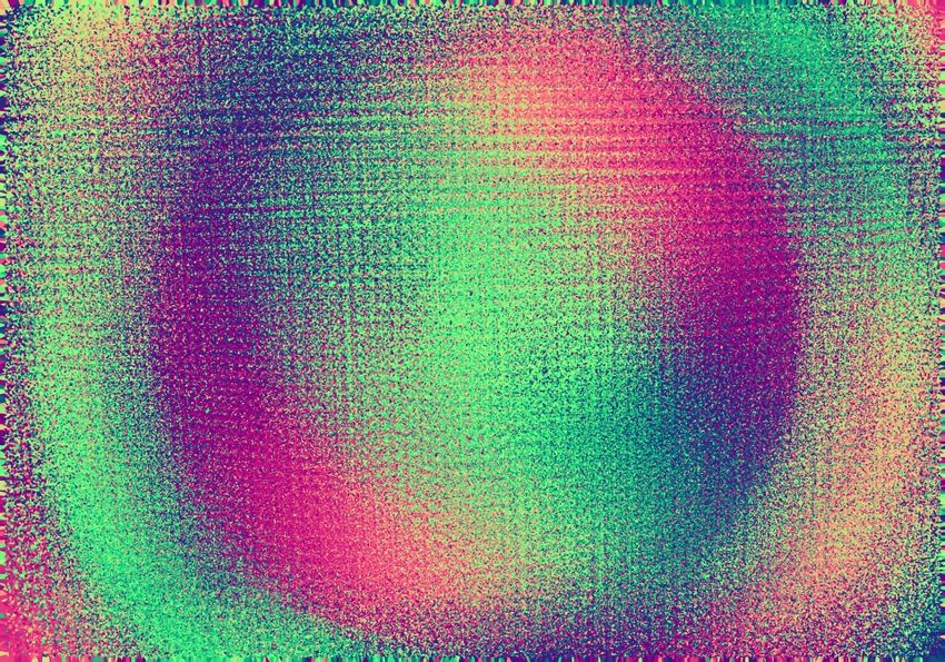
shortly discuss the performance of our camera models.             Here, C denotes the set of all cameras, Ic the set of all im-
   For central cameras, images may be ’undistorted’ to a          ages taken by camera c, and Oi the feature observations in
different camera model, usually the pinhole model. This           image i. po is the 3D pattern point corresponding to obser-
transformation can be cached for calibrated cameras; once         vation o, and di,o the 2D detection of this point in image i.
a lookup table for performing it is computed, the choice          Ti is the pose of image i which transforms global 3D points
of the original camera model has no influence on the run-         into the local rig frame, and Mc transforms points within
time anymore. For high-field-of-view cameras, e.g., fisheye       the local rig frame into camera c’s frame. πc then projects
cameras, where undistortion to a pinhole model is impracti-       the local point to camera c’s image using the current esti-
cal, one may use lookup tables from pixels to directions and      mate of its calibration. ρ is a loss function on the squared
vice versa. Thus, with an optimized implementation, there         residual; we use the robust Huber loss with parameter 1.
should be either zero or very little performance overhead
                                                                      As is common, we optimize cost C with the Levenberg-
when using generic models for central cameras.
                                                                  Marquardt method, and use local updates for orientations.
   For non-central cameras, image undistortion is not possi-
                                                                  We also use local updates (x1 , x2 ) for the directions within
ble in general. Un-projection can be computed directly (and
                                                                  the camera model grids: We compute two arbitrary, per-
cached in a lookup table for the whole image). It should
                                                                  pendicular tangents t1 , t2 to each direction g and update
thus not be a performance concern. However, projection
                                                                  it by adding a multiple of each tangent vector and then re-
may be slow; ideally, one would first use a fast approxi-                          g+x1 t1 +x2 t2
                                                                  normalizing: kg+x    1 t1 +x2 t2 k
                                                                                                     . Each grid point thus has a 2D
mate method (such as an approximate parametric model or
lookup table) and then perform a few iterations of optimiza-      update in the central model and a 5D update in the non-
tion to get an accurate result. The performance of this may       central one (two for the direction, and three for a 3D point
highly depend on the ability to quickly obtain good initial       on the line, c.f . Sec. 3.3). The projection π involves an op-
projection estimates for the concrete camera.                     timization process and the Inverse Function Theorem is not
   We think that given appropriate choice of grid resolution,     directly applicable. Thus, we use finite differences to com-
the initial calibration should not take longer than 30 minutes    pute the corresponding parts of the Jacobian.
up to sufficient accuracy on current consumer hardware.               The optimization process in our setting has more dimen-
Parameter choice. The grid resolution is the only param-          sions of Gauge freedom than for typical Bundle Adjustment
eter that must be set by the user. The smallest interesting       problems, which we discuss in the supplemental material.
cell size is similar to the size of the feature refinement win-   We experimented with Gauge fixing, but did not notice an
dow (c.f . Sec. 3.2), since this window will generally ’blur’     advantage to explicitly fixing the Gauge directions; the ad-
details with a kernel of this size. Since we use 21×21 px         dition of the Levenberg-Marquardt diagonal should already
or larger windows for feature extraction, we use grid reso-       make the Hessian approximation invertible.
lutions down to 10 px/cell, which we expect to leave almost           The Levenberg-Marquardt method compares the costs of
no grid-based modeling error. If there is not enough data,        different states to judge whether it makes progress. How-
the resolution should be limited to avoid overfitting.            ever, we cannot always compute all residuals for each state.
3.4. Calibration                                                  During optimization, the projections of 3D points may en-
                                                                  ter and leave the calibrated image area, and since the camera
   Given images with extracted features, and the chosen           model is only defined within this area, residuals cannot be
central or non-central camera model, the model must be cal-       computed for points that do not project into it. If a resid-
ibrated. Our approach is to first initialize a per-pixel model    ual is defined in one state but not in another, how should the
on interpolated pattern matches using [27]. Then we fit the       states be compared in a fair way? A naive solution would be
final model to this, discard the interpolated matches, and        to assign a constant value (e.g., zero) to a residual if it is in-
obtain the final result with bundle adjustment. See [27] and      valid. This causes state updates that make residuals turn in-
the supp. material for details. In the following, we focus on     valid to be overrated, while updates that make residuals turn
the refinement step that is responsible for the final accuracy.   valid will be underrated. As a result, the optimization could
Bundle Adjustment. Bundle adjustment jointly refines the          stall. Instead, we propose to compare states by summing
camera model parameters, image poses (potentially within a        the costs only for residuals which are valid in both states.
fixed multi-camera rig), and the 3D locations of the pattern      This way, cost comparisons are always fair; however, some
features. We optimize for the reprojection error, which is        residuals may not be taken into account. Theoretically, this
the standard cost function in bundle adjustment [44]:             may lead to oscillation. We however did not observe this in
                          XX X                                    practice, and we believe that if it happens it will most likely
       C(π, M, T, p) =                 ρ(rTc,i,o rc,i,o ) (2)
                                                                  be very close to the optimum, since otherwise the remaining
                           c∈C i∈Ic o∈Oi
                                                                  residuals likely outweigh the few which change validity. In
                 rc,i,o = πc (Mc Ti po ) − di,o                   such a case, it then seems safe to stop the optimization.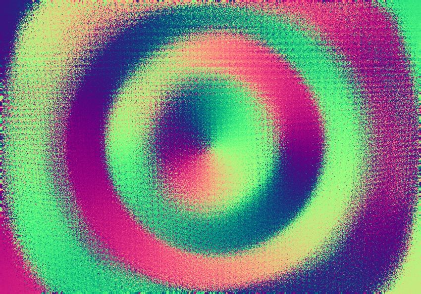
Label  Resolution Field-of-view (FOV)                    Description

                                                                                                   median error [px]
D435-C 1920 × 1080   ca. 70◦ × 42◦                        Color camera of an Intel D435                                                                       X/Y gradients
                                                                                                                       0.10
D435-I 1280 × 800    ca. 90◦ × 64◦                        Infrared camera of an Intel D435                                                                    Gradient magnitudes
 SC-C   640 × 480    ca. 71◦ × 56◦                        Color camera of a Structure Core                                                                    Intensities
                                                                                                                       0.05
 SC-I 1216 × 928     ca. 57◦ × 45◦                        Infrared camera of a Structure Core                                                                 OpenCV cornerSubPix()
                                                                                                                                                              No refinement
Table 1. Specifications of the cameras used in the evaluation                                                          0.00
(more cameras are evaluated in the supplemental material). FOV                                                                D435-C   D435-I   SC-C   SC-I

is measured horizontally and vertically at the center of the image.                               Figure 6. Median reproj. error (y-axis) for calibrating the cameras
                                                                                                  on the x-axis with different feature refinement schemes (colors).
median error [px]

                    0.04                                            0.015     D435-C (31 × 31)    For SC-C, cornerSubPix() results were too inconsistent.
                                                                              D435-C (Deltille)
                    0.03                                                      D435-I (21 × 21)

                    0.02
                                                                    0.010     D435-I (Deltille)   detected in all patterns, for fairness we only keep those fea-
                           4   8   12   16     20
                                         segments
                                                    24   28    32                                 ture detections which succeed for all pattern variants.
Figure 5. Median reprojection errors (y-axis) for calibrating cam-                                    Since there is no ground truth for feature detections, we
eras D435-C and D435-I with patterns having different numbers of                                  compare different patterns via the achieved reprojection er-
star segments (x-axis). The feature refinement window was 31×31                                   rors. We calibrate each set of images of a single pattern
pixels for D435-C and 21×21 pixels for D435-I. The Deltille re-                                   separately and compute its median reprojection error. These
sults were obtained with the feature refinement from [16].                                        results are plotted in Fig. 5. Increasing the number of seg-
4. Evaluation                                                                                     ments starting from 4, the accuracy is expected to improve
                                                                                                  first (since more gradients become available for feature re-
   Tab. 1 lists the cameras used for evaluation. The camera                                       finement) and then worsen (since the monitor and camera
labels from this table will be used throughout the evaluation.                                    cannot resolve the pattern anymore). Both plots follow this
   We evaluate the generic models against two parametric                                          expectation, with the best number of segments being 12
ones, both having 12 parameters, which is a high number                                           resp. 20. The experiment shows that neither the commonly
for parametric models. The first is the model implemented                                         used checkerboard pattern nor the ’deltille’ pattern [16] is
in OpenCV [6] using all distortion terms. The second is                                           optimal for either camera (given our feature refinement).
the Thin-Prism Fisheye model [47] with 3 radial distortion                                        For this paper, we thus default to 16 segments as a good
terms, which was used in a stereo benchmark [37]. We also                                         mean value. The results of [16] have higher error than ours
consider a ”Central Radial” model (similar to [7, 18, 43])                                        for both the checkerboard and ’deltille’ pattern.
based on the OpenCV model, adding the two thin-prism pa-
rameters from the Thin-Prism Fisheye model and replac-                                            4.2. Feature Refinement Evaluation
ing the radial term with a spline with many control points.                                           We compare several variants of our feature refinement
With this, we evaluate how much improvement is obtained                                           (c.f . Sec. 3.2): i) The original version of Eq. (1), and ver-
by better radial distortion modeling only. Note that unfor-                                       sions where we replace the raw intensity values by ii) gra-
tunately, no implementations of complete generic calibra-                                         dient magnitudes, or iii) gradients (2-vectors). In addition,
tion pipelines seemed to be available at the time of writ-                                        we evaluate OpenCV’s [6] cornerSubPix() function,
ing. This makes it hard to compare to other generic calibra-                                      which implements [14]. In all cases, the initial feature po-
tion pipelines; we released our approach as open source to                                        sitions for refinement are given by our feature detection
change this. In addition, since we aim to obtain the most ac-                                     scheme. For each camera, we take one calibration dataset,
curate results possible, and since we avoid synthetic experi-                                     apply every feature refinement scheme on it, and compare
ments as they often do not reflect realistic conditions, there                                    the achieved median reprojection errors. Similarly to the
is no ground truth to evaluate against. However, our main                                         previous experiment, we only use features that are found by
interest is in comparing to the commonly used parametric                                          all methods. The results are plotted in Fig. 6. Intensities
models to show why they should (if possible) be avoided.                                          and X/Y gradients give the best results, with X/Y gradients
                                                                                                  performing slightly better for the monochrome cameras and
4.1. Calibration Pattern Evaluation                                                               intensities performing slightly better for the color cameras.
   We validate our choice of pattern (c.f . Sec. 3.1) by vary-
                                                                                                  4.3. Validation of the Generic Model
ing the number of star segments from 4 to 32 (c.f . Fig. 3).
For the 4-segment checkerboard and 6-segment ’deltille’                                              We validate that the generic models we use (c.f . Sec. 3.3)
[16] patterns, we also compare against the feature refine-                                        can calibrate cameras very accurately by verifying that they
ment from [16]. For each pattern variant, we record calibra-                                      achieve bias-free calibrations: The directions of the final
tion images with the same camera from the same poses. We                                          reprojection errors should be random rather than having the
do this by putting the camera on a tripod and showing the                                         same direction in parts of the image, which would indicate
pattern on a monitor. For each tripod pose that we use, we                                        an inability of the model to fit the actual distortion in these
cycle through all evaluated patterns on the monitor to record                                     areas. Fig. 7 shows these directions for different cameras,
a set of images with equal pose. Since not all features are                                       calibrated with each tested model. We also list the median
OpenCV              Thin-Prism Fisheye Central Radial                Central Generic         Central Generic         Central Generic        Noncentral Generic
            (12 parameters)         (12 parameters)   (258 parameters)               ca. 30 px/cell          ca. 20 px/cell          ca. 10 px/cell          ca. 20 px/cell
 D435-C

 images)
  (968

                                                                                                  4.8k                   10.4k                   40.9k                   25.9k
 Errors1   0.092 / 0.091 / 0.748   0.163 / 0.161 / 1.379   0.068 / 0.070 / 0.968   0.030 / 0.039 / 0.264   0.030 / 0.039 / 0.265   0.029 / 0.040 / 0.252   0.024 / 0.032 / 0.184
 images)
 D435-I
  (1347

                                                                                                  2.5k                    5.3k                   20.5k                   13.3k
 Errors1   0.042 / 0.036 / 0.488   0.032 / 0.026 / 0.365   0.042 / 0.037 / 0.490   0.023 / 0.018 / 0.199   0.023 / 0.018 / 0.198   0.023 / 0.018 / 0.189   0.022 / 0.017 / 0.179
 images)
  (1849
  SC-C

                                                                                                  0.7k                    1.5k                    5.9k                    3.8k
 Errors1   0.083 / 0.085 / 0.217   0.083 / 0.084 / 0.215   0.082 / 0.084 / 0.200   0.069 / 0.072 / 0.055   0.069 / 0.072 / 0.054   0.068 / 0.072 / 0.053   0.065 / 0.069 / 0.040
 images)
  (2434
   SC-I

                                                                                                  2.5k                    5.6k                   21.8k                   14.0k
 Errors1   0.069 / 0.064 / 0.589   0.053 / 0.046 / 0.440   0.069 / 0.064 / 0.585   0.035 / 0.030 / 0.133   0.035 / 0.030 / 0.139   0.034 / 0.030 / 0.137   0.030 / 0.026 / 0.120
            Figure 7. Directions (see legend on the left) of all reprojection errors for calibrating the camera given by the row with the
            model given by the column. Each pixel shows the direction of the closest reprojection error from all images. Ideally, the result
            is free from any systematic pattern. Patterns indicate biased results arising from inability to model the true camera geometry.
                                                                                  1
            Parameter counts for generic models are given in the images.            Median training error [px] / test error [px] / biasedness.

reprojection errors, both on the calibration data and on a                                         D435-C                   D435-I                SC-C               SC-I
test set that was not used for calibration. The latter is used
to confirm that the models do not overfit. As a metric of bi-
asedness, we compute the KL-Divergence between the 2D
normal distribution, and the empirical distribution of repro-
jection error vectors (scaled to have the same mean error
norm), in each cell of a regular 50 × 50 grid placed on the
image. We report the median value over these cells in Fig. 7.                              Figure 8. Differences between calibrations with the central-generic
    The generic models achieve lower errors than the para-                                 model and fitted Thin-Prism Fisheye calibrations, measured as re-
metric ones throughout, while showing hardly any signs of                                  projection errors. Top: Medium gray corresponds to zero error,
overfitting. This is expected, since – given enough calibra-                               while saturated colors as in Fig. 7 correspond to 0.2 pixels differ-
tion images – the whole image domain can be covered with                                   ence. Bottom: Alternative visualization showing the error magni-
training data, thus there will be no ’unknown’ samples dur-                                tude only, with black for zero error and white for 0.2 pixels error.
ing test time. Interestingly, the non-central model consis-
tently performs best for all cameras in every metric, despite
                                                                                           imize the two models’ deviations in the observation direc-
all of the cameras being standard near-pinhole cameras.
                                                                                           tions per-pixel. At the same time, we optimize for a 3D
    All parametric models show strong bias patterns in the                                 rotation applied to the observation directions of one model,
error directions. For some cameras, the generic models also                                since consistent rotation of all image poses for a camera can
show high-frequency patterns with lower grid resolutions                                   be viewed as part of the intrinsic calibration. After conver-
that disappear with higher resolution. These would be very                                 gence, we visualize the remaining differences in the obser-
hard to fit with any parametric model. The central radial                                  vation directions. While these visualizations will naturally
model only improves over the two parametric models for                                     be similar to those of Fig. 7 given our model is very accu-
one camera, showing that improved radial distortion model-                                 rate, we can avoid showing the feature detection noise here.
ing alone is often not sufficient for significant improvement.                             Here, we visualize both direction and magnitude of the dif-
                                                                                           ferences, while Fig. 7 only visualizes directions. The results
4.4. Comparison of Different Models
                                                                                           are shown in Fig. 8, and confirm that the models differ in
   We now take a closer look at the differences between                                    ways that would be difficult to model with standard para-
accurate calibrations and calibrations obtained with typical                               metric models. Depending on the camera and image area,
parametric models. We fit the Thin-Prism Fisheye model to                                  the reprojection differences are commonly up to 0.2 pixels,
our calibrations, optimizing the model parameters to min-                                  or even higher for the high-resolution camera D435-C.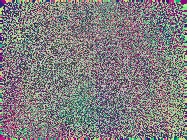
sponding points in the aligned clouds. Depending on the
                                                                  image area, the error is often about half a centimeter, and
                                                                  goes up to more than 1 cm for both cameras. This matches
                                                                  the theoretical result from above well and shows that one
                                                                  should avoid such a bias for accurate results.
              D435                      Structure Core            4.6. Example Application: Camera Pose Estimation
Figure 9. Distances (black: 0cm, white: 1cm) between corre-          To provide a broader picture, we also consider camera
sponding points estimated by dense stereo with a generic and a
                                                                  pose estimation as an application. For this experiment,
parametric calibration, at roughly 2 meters depth.
                                                                  we treat the central-generic calibration as ground truth and
4.5. Example Application: Stereo Depth Estimation                 sample 15 random pixel locations in the image. We un-
                                                                  project each pixel to a random distance to the camera from
   So far, we showed that generic models yield better cal-
                                                                  1.5 to 2.5 meters. Then we change to the Thin-Prism Fish-
ibrations than common parametric ones. However, the dif-
                                                                  eye model and localize the camera with the 2D-3D corre-
ferences might appear small, and it might thus be unclear
                                                                  spondences defined above. The median error in the esti-
how valuable they are in practice. Thus, we now look at the
                                                                  mated camera centers is 2.15 mm for D435-C, 0.25 mm for
role of small calibration errors in example applications.
                                                                  D435-I, 1.80 mm for SC-C, and 0.76 mm for SC-I.
   Concretely, we consider dense depth estimation for the
                                                                     Such errors may accumulate during visual odometry or
Intel D435 and Occipital Structure Core active stereo cam-
                                                                  SLAM. To test this, we use Colmap [35] on several videos
eras. These devices contain infrared camera pairs with a rel-
                                                                  and bundle-adjust the resulting sparse reconstructions both
atively small baseline, as well as an infrared projector that
                                                                  with our Thin-Prism-Fisheye and non-central generic cali-
provides texture for stereo matching. The projector behaves
                                                                  brations. For each reconstruction pair, we align the scale
like an external light and thus does not need to be calibrated;
                                                                  and the initial camera poses of the video, and compute the
only the calibration of the stereo cameras is relevant.
                                                                  resulting relative translation error at the final image com-
   Based on the previous experiments, we make the conser-
                                                                  pared to the trajectory length. For camera D435-I, we obtain
vative assumption that the calibration error for parametric
                                                                  1.3% ± 0.3% error, while for SC-C, we get 5.6% ± 2.2%.
models will be at least 0.05 pixels in many parts of the im-
                                                                  These errors strongly depend on the camera, reconstruction
age. Errors in both stereo images may add up or cancel
                                                                  system, scene, and trajectory, so our results only represent
each other out depending on their directions. A reasonable
                                                                  examples. However, they clearly show that even small cali-
assumption is that the calibration error will lead to a dispar-
                                                                  bration improvements can be significant in practice.
ity error of similar magnitude. Note that for typical stereo
systems, the stereo matching error for easy-to-match sur-         5. Conclusion
faces may be assumed to be as low as 0.1 pixels [36]; in this        We proposed a generic camera calibration pipeline
case, the calibration error may even come close to the level      which focuses on accuracy while being easy to use. It
of noise. The well-known relation between disparity x and         achieves virtually bias-free results in contrast to using
depth d is: d = bf                                                parametric models; for all tested cameras, the non-central
                   x , with baseline b and focal length f . Let
us consider b = 5cm and f = 650px (roughly matching               generic model performs best. We also showed that even
the D435). For d = 2m for example, a disparity error of           small calibration improvements can be valuable in practice,
±0.05px results in a depth error of about 0.6cm. This error
                                                                  since they avoid biases that may be hard to average out.
                                                                     Thus, we believe that generic models should replace
grows quadratically with depth, and since it stays constant
                                                                  parametric ones as the default solution for camera calibra-
over time, it acts as a bias that will not easily average out.    tion. If a central model is used, this might not even intro-
   For empirical validation, we calibrate the stereo pairs of     duce a performance penalty, since the runtime performance
a D435 and a Structure Core device with both the central-         of image undistortion via lookup does not depend on the
generic and the Thin-Prism Fisheye model (which fits the          original model. We facilitate the use of generic models
D435-I and SC-I cameras better than the OpenCV model,             by releasing our calibration pipeline as open source. How-
see Fig. 7). With each device, we recorded a stereo image of      ever, generic models might not be suitable for all use cases,
a roughly planar wall in approx. 2m distance and estimated        in particular if the performance of projection to distorted
a depth image for the left camera with both calibrations.         images is crucial, if self-calibration is required, or if not
Standard PatchMatch Stereo [4] with Zero-Mean Normal-             enough data for dense calibration is available.
ized Cross Correlation costs works well given the actively        Acknowledgements. Thomas Schöps was partially supported
projected texture. The resulting point clouds were aligned        by a Google PhD Fellowship. Viktor Larsson was supported by
with a similarity transform with the Umeyama method [45],         the ETH Zurich Postdoctoral Fellowship program. This work was
since the different calibrations may introduce scale and ori-     supported by the Swedish Foundation for Strategic Research (Se-
entation differences. Fig. 9 shows the distances of corre-        mantic Mapping and Visual Navigation for Smart Robots).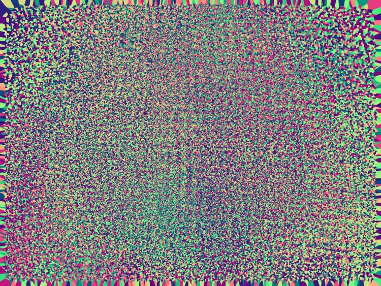
Supplemental Material for:
  Why Having 10,000 Parameters in Your Camera Model is Better Than Twelve

             Thomas Schöps1           Viktor Larsson1     Marc Pollefeys1,2     Torsten Sattler3
                                    1
                                   Department of Computer Science, ETH Zürich
                             2
                               Microsoft, Zurich 3 Chalmers University of Technology

   In this supplemental material, we present additional in-                known pattern               rendering                 image
formation that did not fit into the paper for space reasons.
In Sec. 6, we present the feature detection process that we
use to find the approximate locations of star center features
in images of our calibration pattern. In Sec. 7, we present                                (a)                         (b)
the initialization process for camera calibration. In Sec. 8,
we discuss additional details of our bundle adjustment. In
Sec. 9, we show results of the camera model validation ex-              Figure 10. Sketch of matching-based feature refinement. (a)
periment for more cameras. In Sec. 10, we present more                  Based on an estimate for a local homography between the pattern
details of the results of the Structure-from-Motion experi-             and the image, the known pattern is rendered with supersampling
                                                                        (subpixels illustrated for center sample only for clarity). The result
ment that tests the impact of different camera models in an
                                                                        are rendered grayscale samples shown in the center. (b) The sam-
application context.                                                    ples are (rigidly) moved within the image to find the best match-
                                                                        ing feature position, while accounting for affine brightness differ-
6. Feature detection                                                    ences.

   First, we find all AprilTags in the image using the April-
Tag library [46]. The four corners of each detected April-              tions, before we apply an accurate refinement step with a
Tag provide correspondences between the known calibra-                  smaller convergence region afterwards.
tion pattern and the image. We use these to compute a                   Matching-based refinement and validation. The goal of
homography that approximately maps points on the pattern                matching-based refinement is to improve an initial feature
into the image. This will only be perfectly accurate for pin-           position estimate and reject wrong estimates. As input, the
hole cameras and planar patterns. However, in general it                process described above yields an initial rough estimate of
will be locally appropriate next to the correspondences that            the feature position and a homography that locally approx-
were used to define the homography. With this, we roughly               imates the mapping between the known calibration pattern
estimate the positions of all star features that are directly ad-       and the image. The matching process uses the homography
jacent to an AprilTag. Each feature location is then refined            to render a synthetic image of the pattern in a small win-
and validated with the refinement process detailed below.               dow around the feature position. Then it locally optimizes
After refinement, the final feature positions provide addi-             the alignment between this rendering and the actual image.
tional correspondences between the pattern and the image.               This is illustrated in Fig. 10.
For each newly detected and refined feature location, we                    In detail, we define a local window for refinement, for
compute a new local homography from the correspondences                 which we mostly use 21×21 pixels. The optimum size de-
that are closest to it in order to predict its remaining adja-          pends on many factors such as the blur introduced by out-
cent feature locations that have not been detected yet. We              of-focus imaging, internal image processing in the camera,
then repeat the process of feature refinement, local homog-             and clarity of the calibration pattern. It is thus a parame-
raphy estimation, and growing, until no additional feature              ter that should be tuned to the specific situation. Within this
can be detected.                                                        window, we sample as many random points as there are pix-
   The initial feature locations predicted by the above pro-            els in the window. We assume that the window is centered
cedure can be relatively inaccurate. Thus, we first apply a             on the feature location, and given the local homography es-
well-converging matching process based on the known pat-                timate, we determine the intensity that would be expected
tern appearance to refine and validate the feature predic-              for a perfect pattern observation at each sample location.

                                                                    9
We use 16x supersampling to more accurately predict the            planar, we can use a homography to approximately map be-
intensities.                                                       tween the pattern and the image (neglecting lens distortion).
    Next, we match this rendering with the actual image ob-        Each square of four adjacent feature positions is used to de-
servation by optimizing for a 2-dimensional translational          fine a homography, which we use for mapping within this
shift x of all samples in the image. In addition, since the        square. This allows to obtain dense approximate pattern co-
black and white parts of the pattern will rarely be perfectly      ordinates for all image pixels at which the pattern is visible.
black and white under real imaging conditions, we optimize         These approximately interpolated matches are only used for
for an affine brightness transform to bring the sample in-         initialization, not for the subsequent refinement.
tensities and image intensities into correspondence. In to-            We then randomly sample up to 500 image triples from
tal, we thus optimize for four parameters with the following       the set of all available images. We score each triple based on
cost function:                                                     the number of pixels that have a dense feature observation in
                            n                                      each of the three images. The image triple with the highest
                            X                        2
       Cmatch (x, f, b) =       (f · pi (x) + b − qi )   ,   (3)   number of such pixels is used for initialization.
                            i                                          Since all tested cameras were near-central, we always
                                                                   assume a central camera during initialization (and switch to
where f and b are the affine factor and bias, pi (x) is the bi-    the non-central model later if requested). We thus use the
linearly interpolated image intensity at the sample position       linear pose solver for central cameras and planar calibration
i with the current translation shift x, and qi is the rendered     targets from [27]. For each image pixel which has an (in-
intensity of sample i. Given the initial translation offset        terpolated) feature observation in each of the three images
x = 0, we can initialize f and b directly by minimizing            chosen above, the corresponding known 3D point on the
Cmatch . Setting both partial derivatives to zero eventually       calibration pattern is inserted into a 3D point cloud for each
yields (dropping i from the notation for brevity):                 image. The initialization approach [27] is based on the fact
                                                                   that for a given observation, the corresponding points in the
           (qp) − n1
         P           P P
                        p q
                                        P         P
                                           q−f p                   three point clouds must lie on the same line in 3D space. It
   f= P                         ,  b =                  . (4)
            (pp) − n1 ( p)2                   n
                       P
                                                                   solves for an estimate of the relative pose of the three ini-
                                                                   tial images, and the position of the camera’s optical center.
Subsequently, we optimize all four parameters with the             This allows to project the pattern into image space for each
Levenberg-Marquardt method. The factor parameter f is              pixel with a matched pattern coordinate, which initializes
not constrained in this optimization and may become nega-          the observation direction for these pixels.
tive, indicating that we have likely found a part of the image
                                                                       Next, we extend the calibration by localizing additional
that looks more like the inverse of a feature than the fea-
                                                                   images using the calibration obtained so far with standard
ture itself. While this may appear like a deficiency, since
                                                                   techniques [21]. Each localized image can be used to
pushing the parameter to be positive might have nudged the
                                                                   project the calibration pattern into image space, as above,
translation x to go towards the proper feature instead, we
                                                                   and extend the calibrated image region. For pixels that al-
can actually use it to our advantage, as we can use the con-
                                                                   ready have an estimate of their observation direction, we
dition of f to be positive as a means to reject outliers. This
                                                                   use the average of all directions to increase robustness. If
allows us to obtain virtually outlier-free detections.
                                                                   more than one calibration pattern is used, we can determine
    Note that for performance reasons, in this part of the re-
                                                                   the relative pose between the targets from images in which
finement we do not optimize for the full homography that
                                                                   multiple targets are visible. We localize as many images as
is used at the start to render the pattern prediction. This
                                                                   possible with the above scheme.
changes in the following symmetry-based refinement step,
                                                                       As a result, we obtain a per-pixel camera model which
which is described in Sec. 3.2 in the paper.
                                                                   stores an observation direction for each initialized pixel.
                                                                   We then fit the final camera model to this initialization
7. Calibration initialization
                                                                   by first setting the direction of each grid point in the fi-
   In this section, we describe how we obtain an initial cam-      nal model to the direction of its corresponding pixel in the
era calibration that is later refined with bundle adjustment,      per-pixel model. If the pixel does not have a direction esti-
as described in the paper.                                         mate, we guess it based on the directions of its neighbors.
   For each image, we first interpolate the feature detec-         Finally, using a non-linear optimization process with the
tions over the whole pattern area for initialization purposes,     Levenberg-Marquardt method, we optimize the model pa-
as in [27]. This is important to get feature detections at         rameters such that the resulting observation directions for
equal pixels in different images, which is required for the        each pixel match the per-pixel initialization as closely as
relative pose initialization approach [27] that is used later.     possible.
Since we know that the calibration pattern is approximately            Due to the size of the local window in feature refinement
Used Field-of-view (FOV)
Label resolution (approximate) Type Description
D435-C 1920 × 1080 70◦ × 42◦ RGB Color camera of an Intel RealSense D435
D435-I 1280 × 800 90◦ × 64◦ Mono Infrared camera of an Intel RealSense D435
SC-C 640 × 480 71◦ × 56◦ RGB Color camera of an Occipital Structure Core (color version)
SC-I 1216 × 928 57◦ × 45◦ Mono Infrared camera of an Occipital Structure Core (color version)
Tango 640 × 480 131◦ × 99◦ Mono Fisheye camera of a Google Tango Development Kit Tablet
FPGA 748 × 468 111◦ × 66◦ Mono Camera attached to an FPGA
GoPro 3000 × 2250 123◦ × 95◦ RGB GoPro Hero4 Silver action camera
HTC One M9 3840 × 2688 64◦ × 47◦ RGB Main (back) camera of an HTC One M9 smartphone
Table 2. Specifications of the cameras used in the evaluation: The resolution at which we used them, and the approximate field-of-view,
which is measured horizontally and vertically at the center of the image. SC-I provides images that are pre-undistorted by the camera.
(c.f . the section on feature extraction in the paper), features need to contain feature detections to be well-constrained
cannot be detected close to the image borders (since the (which is again most difficult for the image corners).
window would leave the image). We thus restrict the fitted
model to the axis-aligned bounding rectangle of the feature 9. Camera model validation
observations.
Fig. 11 extends Fig. 7 in the paper with results for ad-
ditional cameras. The specifications of all cameras in the
8. Bundle adjustment details figure are given in Tab. 2. Note that the “Tango” camera
has a fisheye lens and shows hardly any image information
Gauge freedom. As mentioned in the paper, in our set- in the corners. Thus, there are no feature detections in the
ting there are more dimensions of Gauge freedom than for image corners, which causes large Voronoi cells to be there
typical Bundle Adjustment problems. Note that we do not in Fig. 11.
use any scaling information for the pattern(s) during bun-
dle adjustment, but scale its result once as a post-processing 10. Example Application: Camera Pose Esti-
step based on the known physical pattern size. For the cen-
tral camera model, the Gauge freedom dimensions are thus:
mation
3 for global translation, 3 for global rotation, 1 for global In Fig. 12, we present example images of the sparse 3D
scaling, and 3 for rotating all camera poses in one direc- reconstructions that we evaluated in the paper to determine
tion while rotating all calibrated observation directions in how much the results of bundle adjustment in Structure-
the opposite direction. For the non-central camera model, from-Motion are affected by the choice of camera model.
the Gauge freedom dimensions are those listed for the cen- The videos used for these reconstructions were recorded
tral model and additionally 3 for moving all camera poses with the SC-C and D435-I cameras by walking in a mostly
in one direction while moving all calibrated lines in the op- straight line on a forest road, looking either sideways or for-
posite direction. Furthermore, if the calibrated lines are ward. For D435-I, we use 10 videos with 100 frames each,
(nearly) parallel, there can be more directions, since then whereas for SC-C, we use 7 videos with 264 frames on av-
the cost will be invariant to changes of the 3D line origin erage.
points within the lines.
Calibration data bias. For parametric models, whose pa-
rameters affect the whole image area, different densities in
detected features may introduce a bias, since the camera
model will be optimized to fit better to areas where there
are more feature detections than to areas where there are
less. Note that this is a reason for image corners typically
being modeled badly with these models, since there typi-
cally are very few observations in the corners compared to
the rest of the image, and the corners are at the end of the
range of radius values that are relevant for radial distortion.
For our generic models, while there is some dependence
among different image areas due to interpolation within the
grid, they are mostly independent. Thus, this kind of cal-
ibration data bias should not be a concern for our models.
However, unless using regularization, all parts of the imageOpenCV Thin-Prism Fisheye Central Radial Central Generic Central Generic Central Generic Noncentral Generic
(12 parameters) (12 parameters) (258 parameters) ca. 30 px/cell ca. 20 px/cell ca. 10 px/cell ca. 20 px/cell
D435-C
images)
(968
4.8k 10.4k 40.9k 25.9k
Errors1 0.092 / 0.091 / 0.748 0.163 / 0.161 / 1.379 0.068 / 0.070 / 0.968 0.030 / 0.039 / 0.264 0.030 / 0.039 / 0.265 0.029 / 0.040 / 0.252 0.024 / 0.032 / 0.184
images)
D435-I
(1347
2.5k 5.3k 20.5k 13.3k
Errors1 0.042 / 0.036 / 0.488 0.032 / 0.026 / 0.365 0.042 / 0.037 / 0.490 0.023 / 0.018 / 0.199 0.023 / 0.018 / 0.198 0.023 / 0.018 / 0.189 0.022 / 0.017 / 0.179
images)
(1849
SC-C
0.7k 1.5k 5.9k 3.8k
Errors1 0.083 / 0.085 / 0.217 0.083 / 0.084 / 0.215 0.082 / 0.084 / 0.200 0.069 / 0.072 / 0.055 0.069 / 0.072 / 0.054 0.068 / 0.072 / 0.053 0.065 / 0.069 / 0.040
images)
(2434
SC-I
2.5k 5.6k 21.8k 14.0k
Errors1 0.069 / 0.064 / 0.589 0.053 / 0.046 / 0.440 0.069 / 0.064 / 0.585 0.035 / 0.030 / 0.133 0.035 / 0.030 / 0.139 0.034 / 0.030 / 0.137 0.030 / 0.026 / 0.120
images)
Tango
(2293
0.7k 1.6k 6.0k 4.0k
Errors1 0.067 / 0.062 / 0.776 0.034 / 0.031 / 0.367 0.033 / 0.029 / 0.331 0.022 / 0.021 / 0.130 0.022 / 0.021 / 0.127 0.022 / 0.021 / 0.125 0.020 / 0.019 / 0.131
images)
FPGA
(2142
0.8k 1.8k 6.8k 4.6k
Errors1 0.024 / 0.022 / 0.442 0.019 / 0.018 / 0.379 0.021 / 0.019 / 0.317 0.016 / 0.015 / 0.091 0.016 / 0.015 / 0.091 0.015 / 0.015 / 0.091 0.012 / 0.012 / 0.044
Central Generic Central Generic Central Generic Noncentral Generic
OpenCV Thin-Prism Fisheye Central Radial ca. 60 px/cell ca. 50 px/cell ca. 40 px/cell ca. 50 px/cell
images)
GoPro
(440
3.9k 5.4k 8.4k 13.5k
Errors1 0.113 / 0.115 / 0.819 0.105 / 0.108 / 0.773 0.106 / 0.108 / 0.759 0.091 / 0.095 / 0.676 0.091 / 0.095 / 0.679 0.091 / 0.096 / 0.672 0.060 / 0.066 / 0.642
HTC One M9
images)
(195
6.0k 8.6k 13.2k 21.4k
Errors1 0.178 / 0.161 / 1.174 0.360 / 0.298 / 1.830 0.089 / 0.095 / 0.694 0.043 / 0.045 / 0.378 0.043 / 0.045 / 0.378 0.043 / 0.045 / 0.377 0.039 / 0.039 / 0.352
Figure 11. Directions (encoded as colors, see legend on the left) of all reprojection errors for calibrating the camera
defined by the row with the model defined by the column. Each pixel shows the direction of the closest reprojection
error (i.e., the images are Voronoi diagrams) from all used images. Ideally, the result is free from any systematic
pattern. Patterns indicate biased results arising from not being able to model the true camera. Parameter counts for
1
generic models are given in the images. Median training error [px] / test error [px] / biasedness.You can also read