Can wave coupling improve operational regional ocean forecasts for the north-west European Shelf? - Ocean Science
←
→
Page content transcription
If your browser does not render page correctly, please read the page content below

Ocean Sci., 15, 669–690, 2019
https://doi.org/10.5194/os-15-669-2019
© Author(s) 2019. This work is distributed under
the Creative Commons Attribution 4.0 License.

Can wave coupling improve operational regional ocean forecasts
for the north-west European Shelf?
Huw W. Lewis1 , Juan Manuel Castillo Sanchez1 , John Siddorn1 , Robert R. King1 , Marina Tonani1 , Andrew Saulter1 ,
Peter Sykes1 , Anne-Christine Pequignet1 , Graham P. Weedon1 , Tamzin Palmer1 , Joanna Staneva2 , and
Lucy Bricheno3
1 Met Office, Exeter, EX1 3PB, UK
2 Institute
          for Coastal Research, Helmholtz-Zentrum Geesthacht, Max-Planck-Strasse 1, 21502 Geesthacht, Germany
3 National Oceanography Centre, Joseph Proudman Building, 6 Brownlow Street, Liverpool, L3 5DA, UK

Correspondence: Huw W. Lewis (huw.lewis@metoffice.gov.uk)

Received: 18 December 2018 – Discussion started: 21 December 2018
Revised: 11 April 2019 – Accepted: 6 May 2019 – Published: 5 June 2019

Abstract. Operational ocean forecasts are typically produced    ational implementation. When results are considered in more
by modelling systems run using a forced mode approach.          depth, wave coupling was found to result in an annual cycle
The evolution of the ocean state is not directly influenced     of relatively warmer winter and cooler summer sea surface
by surface waves, and the ocean dynamics are driven by an       temperatures for seasonally stratified regions of the NWS.
external source of meteorological data which are indepen-       This is driven by enhanced mixing due to waves, and a deep-
dent of the ocean state. Model coupling provides one ap-        ening of the ocean mixed layer during summer. The impact of
proach to increase the extent to which ocean forecast systems   wave coupling is shown to be reduced within the mixed layer
can represent the interactions and feedbacks between ocean,     with assimilation of ocean observations. Evaluation of salin-
waves, and the atmosphere seen in nature. This paper demon-     ity and ocean currents against profile measurements in the
strates the impact of improving how the effect of waves on      German Bight demonstrates improved simulation with wave
the momentum exchange across the ocean–atmosphere inter-        coupling relative to control simulations. Further, evidence is
face is represented through ocean–wave coupling on the per-     provided of improvement to simulation of extremes of sea
formance of an operational regional ocean prediction system.    surface height anomalies relative to coastal tide gauges.
This study focuses on the eddy-resolving (1.5 km resolution)
Atlantic Margin Model (AMM15) ocean model configura-
tion for the north-west European Shelf (NWS) region.
   A series of 2-year duration forecast trials of the Coper-    1   Introduction
nicus Marine Environment Monitoring Service (CMEMS)
north-west European Shelf regional ocean prediction sys-        There is a growing understanding of the role that ocean sur-
tem are analysed. The impact of including ocean–wave feed-      face waves play in the Earth system, modulating the ex-
backs via dynamic coupling on the simulated ocean is dis-       change of momentum, energy, and other fluxes between the
cussed. The main interactions included are the modification     atmosphere and oceans (Cavaleri et al., 2012). A key effect
of surface stress by wave growth and dissipation, Stokes–       is in absorbing momentum and energy from the atmosphere
Coriolis forcing, and wave-height-dependent ocean surface       as waves grow, and releasing it to the ocean when they break.
roughness. Given the relevance to operational forecasting,          Prediction systems of the ocean, waves, or atmosphere
trials with and without ocean data assimilation are consid-     have typically been developed in relative isolation and with
ered.                                                           little or no interaction between each component. However,
   Summary forecast metrics demonstrate that the ocean–         the development of coupled prediction approaches is increas-
wave coupled system is a viable evolution for future oper-      ingly enabling research on the sensitivity of the Earth sys-
                                                                tem to wave impacts (e.g. Pullen et al., 2017). Through ex-

Published by Copernicus Publications on behalf of the European Geosciences Union.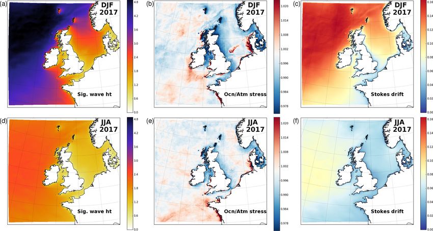
670                                 H. W. Lewis et al.: Can wave coupling improve operational regional ocean forecasts?

change of information between different model components,        Stokes–Coriolis forcing was found to have relatively little
coupled systems can begin to explicitly represent the feed-      impact on the large-scale validation. A clear future develop-
backs and interactions that occur across the air–sea interface   ment for this system would be to move from wave forcing to
in nature. The next evolution in the development of coupled      dynamic coupling in order to allow the ocean and wave states
models is in their application to provide improved forecast      to feed back on each other during the simulation.
information to a range of users through operational ocean           Cavaleri et al. (2018) argue that the interaction of waves
prediction systems.                                              with the ocean is particularly critical in coastal and in-
   This paper discusses the implementation of surface wave       ner seas, as typically simulated using limited-area or re-
effects in an eddy-resolving regional ocean forecasting sys-     gional ocean model domains. This results from the preva-
tem of the north-west European Shelf (NWS) through dy-           lence of younger, steeper, and shorter-wavelength waves that
namic ocean–wave coupling. The ocean model configuration         are more sensitive to variability in the near-surface wind and
is the Atlantic Margin Model at 1.5 km resolution (AMM15;        ocean currents, often with non-linear interactions. A number
Graham et al., 2018a). This is currently used operationally as   of studies have assessed the influence of surface waves on re-
part of the Copernicus Marine Environment Monitoring Ser-        gional ocean dynamics, although to date this has often been
vice (CMEMS) in ocean-only mode for which external forc-         through a case study approach rather than with an operational
ing is provided from a global-scale resolution meteorologi-      focus (Cavaleri et al., 2018).
cal forecast system and the effect of waves is mostly omit-         For example, Clementi et al. (2017) introduced a relatively
ted other than where implicitly captured within the standard     reduced-complexity coupling of the mean momentum trans-
ocean model parameterisations (Tonani et al., 2019, this is-     fer of waves and wind speed stability parameter between
sue).                                                            the WAVEWATCH III wave model (Tolman et al., 2004)
   AMM15 uses the NEMO ocean model (Nucleus for Euro-            and NEMO ocean model codes. They demonstrated that for
pean Modelling of the Ocean; Madec et al., 2016). Breivik        the Mediterranean Sea while the coupling was found to im-
et al. (2015) presented the first discussion of including sur-   prove wave performance, there was limited impact on mean
face wave effects in NEMO based on global-scale ocean            SST results over the 5-year study period. However, focusing
simulations at 1◦ resolution. They included parameterisa-        on a short-range case study period for a strong storm event
tions for the modification of surface stress from wave growth    showed a marked improvement in the evolution of surface
and dissipation (Janssen et al., 2004), the Stokes–Coriolis      currents relative to observations.
force (Hasselmann, 1970), and the turbulent kinetic energy          Some of the earliest studies of wave–ocean interactions
flux from breaking waves (Craig and Banner, 1994). Breivik       for regional seas focused on coastal regions of the UK (e.g.
et al. (2015) demonstrated reduced sea surface and subsur-       Wolf, 2008; Brown and Wolf, 2009; Brown et al., 2011;
face temperature biases relative to observations, and im-        Bricheno et al., 2013; Bolaños et al., 2014) using the POL-
proved predictions of the total ocean heat content at global     COMS ocean (Holt and James, 2001) and WAM (WAMDI,
scales. This led to the operational implementation of wave-      1988) wave models. Brown et al. (2011) presented the sensi-
related processes in a coupled ensemble forecast system at       tivity of results to model resolution during an extreme storm
the European Centre for Medium-Range Weather Forecasts           and found that representing wave–current interactions in a
(ECMWF; e.g. Janssen and Bidlot, 2018). Most recently,           system with 1.8 km horizontal resolution, most analogous to
these feedbacks have been applied within its coupled reanal-     AMM15 used in this study, gave results as good if not better
ysis (Laloyaux et al., 2018).                                    than using a yet higher resolution (180 m grid).
   Law Chune and Aouf (2018) recently discussed the impact          Several studies have applied the Coupled–Ocean–
of these wave effects in a global NEMO ocean model config-       Atmosphere–Wave–Sediment Transport modelling system
uration at higher resolution in the context of aiming to im-     (COAWST; Warner et al., 2010) to assess the impact of wave
prove the performance of the CMEMS global ocean model            and atmosphere coupling on regional ocean dynamics. For
forecast system and showed a significant reduction in sea        example, Bruneau and Toumi (2016) used a regional model
surface temperature (SST) bias focused in tropical regions,      configuration of the Caspian Sea and found that surface wave
driven by the modified momentum flux. In their ocean-only        processes led to enhanced mixing and a relative deepening
control simulation, SST was generally too warm in semi-          of the mixed layer depth, particularly in summer. Carniel et
enclosed seas, including along western European seas. It was     al. (2016) applied COAWST for a cold air outbreak episode
expected that mid-latitude SST would conversely cool due to      over the northern Adriatic Sea and found the interaction with
enhanced stress and mixing, although results showed rela-        waves provided further improved forecast skill beyond that
tively smaller and more variable impacts than in the tropics.    obtained by introducing ocean–atmosphere feedbacks to im-
Law Chune and Aouf (2018) also demonstrated enhanced             prove the simulated heat fluxes. The impacts of wave–ocean
surface current speeds generally, with improved validation       coupling in the absence of atmosphere feedbacks were con-
relative to observations of the order of 5 %. In agreement       sidered by Benetazzo et al. (2014).
with previous work, wave breaking was considered to be the          COAWST has also been implemented for a domain cover-
most important wave process for mid-latitude regions while       ing the north-west European shelf seas by Reza Hashemi et

Ocean Sci., 15, 669–690, 2019                                                               www.ocean-sci.net/15/669/2019/
H. W. Lewis et al.: Can wave coupling improve operational regional ocean forecasts?                                            671

al. (2015), similar to that used in this study, using a horizon-          sights into the impact of coupling in assimilative sys-
tal grid spacing of the order of 4 km (1/24◦ ). Their analysis            tems.
focused on the impact of coupling on the wave simulations
for wave energy resource applications (Hashemi and Lewis,             Note that the studies discussed above were all conducted in
2017). Lewis et al. (2019) used the same COAWST system             the framework of “free running” ocean simulations, with no
for the role of tidal dynamics on the wave climate of the Irish    assimilation of observations active. By explicitly considering
Sea.                                                               the role of ocean assimilation in this study, the likely impact
   Staneva et al. (2017) considered the effect of wave forcing     of coupling on operational forecasts can be assessed.
from the WAM wave model on NEMO simulations (3.7 km                   The rest of this paper is organised as follows. The AMM15
grid resolution) of water level and currents for two extreme       coupled model and assimilation configurations are intro-
storm cases over the North Sea. They found a significant           duced in Sect. 2, along with a discussion of the wave cou-
change in simulated storm surge along southern North Sea           pling experiments. Results from a first-order evaluation of
coasts for each storm, especially in near-coastal areas, and       ocean surface variables against observations are shown in
improved representation of observed vertical current pro-          Sect. 3, and comparison against selected research-mode ob-
files. These changes were also predominantly driven by the         servations is discussed in Sect. 4. Conclusions and proposed
wave-modified surface stress, with a secondary contribution        next steps for the operational system development are high-
from Stokes–Coriolis forcing. Staneva et al. (2016a, b) and        lighted in Sect. 5.
Schloen et al. (2017) considered the impact of ocean–wave
coupling in the near-coastal German Bight region of the
                                                                   2     Modelling and evaluation framework
southern North Sea. Alari et al. (2016) assessed the imple-
mentation of a similar coupled NEMO–WAM system in the              The sensitivity of ocean predictions to the representation of
Baltic Sea. In this region, use of a wave-modified surface         ocean–wave feedbacks is assessed by running a number of
stress led to a relative warming of SST, both due to changes in    simulation experiments, as summarised in Table 1, cover-
advection and turbulent fluxes, which reduced the model bias       ing the 2-year period 2016–2017. Experiments are conducted
compared with observations. The impact of Stokes–Coriolis          with and without ocean data assimilation active and with
feedbacks was constrained to coastal areas.                        and without wave coupling in order to examine the influ-
   The role of wave effects on storm surge in the NWS region       ence of wave coupling in both free-running and assimilative
was also studied by Bertin et al. (2015) for two case studies      systems. This leads to a comparison between four configu-
on the west coast of France in the Bay of Biscay using un-         rations, which for brevity will be referred to in this paper as
structured model grid approaches. For one case, the predicted      FR (no coupling, no assimilation), DA (no coupling, assim-
storm surge was increased by up to 25 % and much improved          ilation), CPL_FR (coupling, no assimilation), and CPL_DA
relative to observations when using a wave-dependent sur-          (coupling and assimilation active).
face stress in the presence of young and steep waves. For a
contrasting case, with larger but more developed waves, cou-       2.1    Regional NEMO ocean model configurations
pling did not improve or degrade the forecast quality substan-
tially.                                                            All simulations have been conducted using the AMM15
   The work presented in this paper aims to inform the fu-         configuration of the NEMO ocean model (Madec et al.,
ture evolution of the operational AMM15 prediction system          2016). Full details on the operational implementation of the
implemented as part of CMEMS. Lewis et al. (2018b) pre-            AMM15 configuration for CMEMS are provided by Tonani
sented some initial results on the impact of wave coupling on      et al. (2019, this issue). The science settings and further back-
ocean results for a similar configuration based on a series of     ground on model performance are detailed by Graham et
month-long duration simulations. This study differs in sev-        al. (2018a, b). Through use of a 1.5 km grid spacing, suf-
eral respects, notably that                                        ficient to resolve the internal Rossby radius on the NWS,
                                                                   it has been demonstrated that AMM15 can represent local-
  i. results are presented from 2-year duration simulation         scale processes such as eddies, fronts, internal tides, and ex-
     trials, enabling more robust statistics to be established     changes across the shelf break.
     across seasonal timescales;                                      Meteorological forcing is provided by interpolation from
 ii. simulation experiments make use of the CMEMS op-              the operational European Centre for Medium-Range Weather
     erational forecast system for the NWS, using the              Forecasts (ECMWF) global forecast data at around 14 km
     same sources and treatment of atmospheric forcing and         horizontal resolution and applied at 3-hourly temporal fre-
     boundary conditions as used in operations;                    quency. Surface forcing is implemented using the CORE
                                                                   bulk parameterisations (Large and Yeager, 2004). All sim-
 iii. comparisons are made between free-running simula-            ulations are initialised from the same initial condition, based
      tions and those including assimilation of in situ, satel-    on a 30-year non-assimilative AMM15 run detailed by Gra-
      lite, and profile ocean observations, enabling new in-       ham et al. (2018a). Lateral boundary conditions for the At-

www.ocean-sci.net/15/669/2019/                                                                    Ocean Sci., 15, 669–690, 2019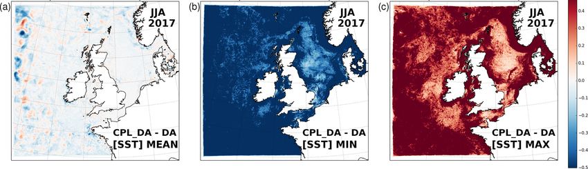
672                                   H. W. Lewis et al.: Can wave coupling improve operational regional ocean forecasts?

Table 1. Overview of simulation experiments conducted.

               Name        Configuration        Wave coupled?      Ocean DA?       Description
               FR          AMM15                no                 no              free-running control simulation
                                                                                   of AMM15
               DA          AMM15_DA             no                 yes             analogous to ocean-only operational
                                                                                   AMM15 system
               CPL_FR      AMM15_CPL            yes                no              free-running ocean–wave coupled
                                                                                   simulation
               CPL_DA      AMM15_CPL_DA         yes                yes             coupled ocean–wave run with ocean
                                                                                   data assimilation

lantic are provided every 3 h from the uncoupled Met Office             influence of the ocean state on wave evolution is already cap-
operational 1/12◦ North Atlantic ocean system (Blockley et              tured in the current operational NWS wave forecasting sys-
al., 2014) and for the Baltic Sea every hour using the oper-            tem through use of previously forecast ocean currents as an
ational Baltic Sea products from CMEMS (Berg and Weis-                  additional external forcing (Palmer and Saulter, 2016).
mann Poulsen, 2012). All simulations are run with a 60 s                   For brevity, the following discussion therefore focuses on
integration time step. Details of the meteorological forcing,           the impact of wave effects on the ocean model results only.
ocean initial condition, and boundary conditions are identical          The case study results presented by Lewis et al. (2018a), for
to those described by Tonani et al. (2019, this issue) and are          example, suggest that the impact of two-way ocean–wave
therefore consistent with the current operational implemen-             feedbacks on wave results is limited compared with includ-
tation of AMM15.                                                        ing ocean processes through external forcing without feed-
   Ocean data assimilation in the DA and CPL_DA runs use                backs, as currently applied in the Met Office operational
the NEMOVAR 3D-variational assimilation scheme (Waters                  wave forecast system.
et al., 2015) which employs a multi-variate balance to ac-
count for correlations between ocean variables as defined               2.3   Wave–ocean coupling
in Weaver et al. (2005). Increments are applied to the 3-D
temperature, salinity, u and v velocities, and the sea sur-             The implementation of wave–ocean coupling in the AMM15
face height (SSH). As detailed by King et al. (2018), assimi-           system follows that described by Lewis et al. (2018b). Cou-
lated observations include in situ and satellite observations of        pling between the ocean and wave model components is
SST and subsurface profile observations of temperature and              achieved by exchanging information between NEMO and
salinity from Argo floats, XBTs (expendable bathythermo-                WAVEWATCH III using the OASIS3-MCT libraries (vn3.0;
graphs), CTDs (conductivity, temperature, and depth), glid-             Valcke et al., 2015). All variables are averaged and ex-
ers, and marine mammals. Sea level anomaly (SLA) obser-                 changed at hourly frequency. Limited-period case study ex-
vations from satellite altimeters are assimilated in the deep           periments using more frequent exchanges have previously
parts of the domain (where the ocean is deeper than 700 m).             suggested that hourly coupling is sufficient to assess the first-
                                                                        order impact of wave coupling on the ocean state.
2.2   Regional WAVEWATCH III wave model                                    The scientific basis for representing wave–ocean inter-
      configuration                                                     actions in AMM15 is described in Sect. 3 of Lewis et
                                                                        al. (2018b), with technical details of the NEMO ocean model
Wave simulations are produced for the NWS using a config-               wave coupling code used in this study provided in Appendix
uration of the WAVEWATCH III (Tolman et al., 2014) spec-                B of Lewis et al. (2018b). This implementation closely
tral wave model (Saulter et al., 2017). The wave model is               follows the work of Breivik et al. (2015) and Staneva et
defined to cover the same domain extent as AMM15, but us-               al. (2017), and for brevity these details are not repeated here.
ing a spherical multiple cell grid refinement approach (Li,             The associated code is now supported for wider use by the
2012), which has variable horizontal resolution nesting from            ocean modelling community from NEMO version 4. In brief,
3 km across much of the domain down to 1.5 km spacing for               the main interactions introduced in the CPL and CPL_DA
all cells adjacent to the coast and/or where the depth of a             experiments are
3 km grid cell would be shallower than 40 m. A wave model
global time step of 600 s is used. The wave model is forced by            a. modification of water-side surface stress on the ocean
winds from the same ECMWF global atmospheric model as                        by wave growth and dissipation (Eq. 3; Lewis et al.,
used for ocean forcing at 3-hourly temporal frequency. The                   2018b);

Ocean Sci., 15, 669–690, 2019                                                                       www.ocean-sci.net/15/669/2019/
H. W. Lewis et al.: Can wave coupling improve operational regional ocean forecasts?                                            673

  b. Stokes–Coriolis force in momentum (Eq. 4; Lewis et al.,       2.4    Wave effects in the NWS
     2018b) and tracer advection equations, using the param-
     eterisation of Breivik et al. (2015);                         As highlighted by a number of studies discussed in the intro-
                                                                   duction, a key driver of ocean dynamics by waves has been
  c. wave-height-dependent ocean surface roughness                 found to be the modification of surface stress. In equilibrium,
     (Eq. 11; Lewis et al., 2018b), following Rascle et            for a fully developed wind-sea state, the input of momentum
     al. (2008).                                                   to surface waves from the wind is matched by its dissipa-
   Note that the wave coupling by Lewis et al. (2018b)             tion into the ocean, and the water-side stress acting at the top
was applied using the direct flux surface forcing scheme of        of the ocean, τocn , is equal to the total atmospheric stress,
NEMO, rather than the CORE bulk forcing used here, and             τatm . For younger, growing waves, there is a net input of mo-
using meteorological forcing from the Met Office Unified           mentum from the atmosphere to waves (τocn τatm ).
zonal and meridional components of the wave-modified sur-          The distribution of τocn /τatm simulated by WAVEWATCH III
face stress (i.e. τocn components) are exchanged directly from     is shown in Fig. 1b and e for summer and winter, respec-
WAVEWATCH III to NEMO, rather than defining a frac-                tively. The magnitude of changes due to waves is shown to be
tion of the total atmospheric stress acting on the ocean as in     larger in winter than summer, although common features can
Breivik et al. (2015). This avoids the need for NEMO to re-        be identified in both seasons. Regions of wave breaking are
calculate the surface stress using a wave-modified drag coef-      identifiable by darker red shading immediately along west-
ficient, thereby removing a source of potential inconsistency      ern coastlines of the UK, France, and Denmark. Waves tend
between the wave and ocean models. However, note that the          to enhance the momentum transferred to the ocean in regions
WAVEWATCH III surface scheme assumes a neutral atmo-               of prevailing wave activity – to the north-west of the NWS
spheric boundary layer, and use of the wave-modified mo-           in winter and more directly west of the NWS in summer.
mentum flux may no longer be in equilibrium with heat and          Momentum transfer is also enhanced on average across the
humidity fluxes. While initial testing (not shown) indicated       Celtic Sea (south-western approaches to the UK) and through
a relatively small effect from the change in representation        the central North Sea, particularly in summer. In contrast, re-
of the surface stress, further work is required to more fully      gions to the lee of land such as through the Irish Sea and to
review the representation of the surface momentum across           the east of the UK are characterised as regions of growing
atmosphere, ocean, and wave model codes.                           waves where momentum is stored in waves rather than trans-
   Only wave effects acting on the ocean momentum budget           ferred from the atmosphere to the ocean (blue areas in Fig. 1b
are considered in this study. Wave impacts on the calcula-         and e).
tion of turbulent heat and moisture fluxes and accounting for         Also shown are seasonal mean distributions of simulated
the wave energy flux transferred to the ocean are omitted. In-     significant wave height (Fig. 1a, d) and Stokes drift speed
stead, the treatment of wave breaking on the surface bound-        (Fig. 1c, f). The Stokes drift speed generally increases with
ary for TKE (turbulent kinetic energy) is parameterised us-        wave height (and forcing wind speed), with highest seasonal
ing the Craig and Banner (1994) scheme, with the default           mean values of up to 16 cm s−1 in regions of greatest wave
value of the Craig and Banner coefficient of 100 used in all       activity across north-western approaches to the UK. There is
simulations. There is also no explicit treatment of Langmuir       also a dependency on water depth, leading to lower values
turbulence, such as through use of a vortex-force formula-         (approximately 5 cm s−1 ) in near-coastal regions.
tion (e.g. Uchiyama et al., 2010), or of ocean bed stress (e.g.
Soulsby et al., 1995), both of which may be important in the
regional ocean context. These simplifications are appropri-        3     Operational-mode ocean metrics
ate for an initial implementation of wave coupling within the
NWS forecast system, given known sensitivities of the verti-       Differences between observed and model values for as-
cal mixing and radiation schemes to parameter choices. Fu-         similated variables (SST, SLA, and profiles of tempera-
ture work will need to reassess model tuning when including        ture and salinity) are calculated in each experiment, from
these additional coupled processes. For example, while sev-        which summary metrics for each 2-year trial can be com-
eral studies have introduced a wave dependence in the TKE          pared. While not fully independent, when assimilation is
parameterisation, the values of this coefficient can be highly     active, differences to observations are computed using the
variable, and further testing will be required to assess a suit-   model background before assimilation (King et al., 2018).
able choice for the range of this parameter in the ocean–wave      Resulting mean difference (MD, expressed here as (Model
coupled system.                                                    Background minus Observation) and root-mean-square dif-
                                                                   ference (RMSD) statistics, averaged across the AMM15 do-
                                                                   main and covering the full 2016–2017 period, are given for
                                                                   SST against in situ data in Table 2 and for SLA in Table 3.

www.ocean-sci.net/15/669/2019/                                                                   Ocean Sci., 15, 669–690, 2019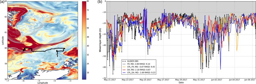
674                                     H. W. Lewis et al.: Can wave coupling improve operational regional ocean forecasts?

Figure 1. Seasonal mean of wave model simulated (a, d) significant wave height, (b, e) fraction of ocean to atmosphere surface stress, and (c,
f) Stokes drift speed during (a–c) winter 2016/2017 and (d–f) summer 2017.

Table 2. SST mean difference (MD = Model minus Observation), and root-mean-square difference (RMSD) statistics computed over 2-year
period (2016–2017) comparing each simulation experiment with available in situ observations. The daily average number of observations
(N) used for each comparison is also listed.

                               SST (MD (K))            FR     CPL_FR         DA     CPL_DA       Daily avg. N
                               Full domain          −0.04        −0.10     0.01         0.01             1100
                               On-shelf regions     −0.14        −0.12     0.03         0.03              540
                               Off-shelf regions     0.07        −0.02    −0.01        −0.01              550
                               SST (RMSD (K))          FR     CPL_FR         DA     CPL_DA       Daily avg. N
                               Full domain            0.64         0.66     0.44         0.44            1100
                               On-shelf regions       0.70         0.72     0.52         0.51             540
                               Off-shelf regions      0.58         0.59     0.35         0.36             550

   In general, the statistics in Tables 2 and 3 show rela-                ference between DA and CPL_DA is negligible, with neither
tively small differences between simulations with and with-               system demonstrating clearly better performance in terms of
out wave coupling. The biggest impact is seen in MD scores                summary metrics.
for SST, with a cold model bias (MD < 0) in the FR results                   Results for SLA comparisons against observations are
made worse with coupling (i.e. in the CPL_FR simulation),                 summarised in Table 3 and are similarly consistent between
for example, from −0.04 to −0.1 K relative to in situ obser-              simulations with and without wave coupling over the 2-year
vations across the full domain. This signal is dominated by               trial period, regardless of whether runs were with or without
compensating biases on and off the shelf in FR (i.e. in shal-             assimilation.
lower and deeper water). When comparing with on-shelf ob-                    A comparison of the variation in mean statistics with depth
servations only, the FR and CPL_FR results are more similar               for simulated temperature and salinity against observed pro-
(MD = −0.14 and −0.12 K, respectively). The correspond-                   files during 2016 and 2017 is shown in Fig. 2. The average
ing difference in RMSD is relatively small (of the order of               temperature error profiles show that, in contrast to SST re-
2 %). When SST observations are assimilated as in the oper-               sults (Table 2), over much of the ocean depth wave feed-
ational CMEMS system, statistics are improved and the dif-                backs result in warming (model increasingly larger than ob-

Ocean Sci., 15, 669–690, 2019                                                                           www.ocean-sci.net/15/669/2019/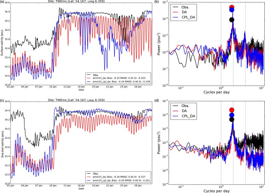
H. W. Lewis et al.: Can wave coupling improve operational regional ocean forecasts?                                                   675

Table 3. SLA mean difference (MD = Model minus Observation) and root-mean-square difference (RMSD) statistics computed over the
2-year period (2016–2017) comparing each simulation experiment with satellite altimeter observations. Results are listed separately for the
full model domain and discriminating between areas on-shelf and off-shelf.

                              SLA (MD (m))             FR    CPL_FR           DA   CPL_DA      Daily avg. N
                              Full domain          −0.01       −0.01     −0.01        −0.01            2000
                              On-shelf regions      0.02        0.02     −0.03        −0.03             670
                              Off-shelf regions    −0.03       −0.02      0.00         0.00            1340
                              SLA (RMSD (m))           FR    CPL_FR           DA   CPL_DA      Daily avg. N
                              Full domain            0.11        0.11       0.11        0.11           2000
                              On-shelf regions       0.13        0.13       0.13        0.13            670
                              Off-shelf regions      0.10        0.10       0.09        0.09           1340

Figure 2. Vertical profiles of (dashed lines) Observation minus Model differences and (solid lines) RMSD statistics for ocean-only and
coupled simulations, computed over 2-year simulation period (2016–2017) for (a, b) temperature and (c, d) salinity, comparing runs (a, c)
with and (b, d) without assimilation.

servations). Over all depths, the RMSD is marginally lower              presents a more detailed analysis of the impact of wave cou-
for CPL_FR than FR (Fig. 2b), and this impact is preserved              pling across the NWS in the AMM15 system.
across most depths in the comparison of CPL_DA with DA
in Fig. 2a. Salinity error profiles (Fig. 2c, d) are unaffected
by coupling away from the surface layers, where the RMSD                4     Sensitivity of ocean state to wave feedbacks
for CPL_FR is on average slightly reduced relative to FR.
However, this impact is greatly reduced when comparing the              4.1    Sea surface temperature (SST)
assimilative results.
   Given that wave coupling has been applied in a system                The impact of wave coupling on simulated SST, in the ab-
that has been optimised to run operationally in an uncou-               sence of data assimilation, is shown in Fig. 3 as seasonal
pled mode (most analogous to the DA configuration here)                 mean differences between FR and CPL_FR through the
with no subsequent tuning of the ocean model physics or as-             2016–2017 trial period. Figure 3 shows substantial spatial
similation, it is encouraging that these summary results are            and temporal variability in mean differences due to wave ef-
generally neutral. This indicates that the addition of coupled          fects in the eddy-dominated deeper ocean off the NWS to the
wave processes is a viable evolution for the NWS forecast               west of the model domain. In contrast, results on the shallow
system and an initial operational implementation would not              NWS show relatively little inter-annual variation in the im-
be anticipated to degrade forecast quality in terms of sum-             pact of coupling, with a consistent spatial distribution of dif-
mary verification metrics. However, as discussed by Tonani              ferences for a given season in both 2016 and 2017. Figure 3b
et al. (2019, this issue) for example, ocean model assessment           also highlights that the impact of wave coupling takes rela-
in terms of such metrics does not provide a sufficient eval-            tively little time to spin up from common initial conditions
uation of the system, particularly when considering regional            in January 2016. For brevity, the subsequent analysis there-
configurations at eddy-resolving scales. Section 4 therefore            fore focuses on results from winter 2016/2017 and spring,

www.ocean-sci.net/15/669/2019/                                                                          Ocean Sci., 15, 669–690, 2019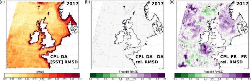
676                                     H. W. Lewis et al.: Can wave coupling improve operational regional ocean forecasts?

Figure 3. (a) Illustration of AMM15 model bathymetry (see Tonani et al., 2019, for more details) and location of NWS observing sites
referenced in the paper. The filled-shading region indicates where model bathymetry in less than 200 m depth and highlights the region on
the shelf. Elsewhere contour lines are drawn every 500 m depth. Filled circles are at “Celtic Sea”, “Perranporth” and “North Sea” sites (see
Sect. 4.1, 4.3). Starred locations in the German Bight are listed in the legend (see Sect. 4.2, 4.4). The yellow square is the “Sheerness” tide
gauge (see Sect. 4.5). (b–h) Difference in seasonal mean SST (CPL_FR minus FR) due to wave coupling calculated as 3-month means from
spring 2016 to autumn 2017.

summer, and autumn 2017 only as being representative, and                    While the main sensitivity of SST to wave coupling on the
results on the NWS as being of primary interest to users of               NWS can be characterised as a net warming in the winter and
operational forecast data in this region.                                 cooling in the summer, closer examination shows this pattern
   Away from the immediate vicinity of coastlines, an annual              can be reversed in the immediate vicinity of some coasts.
cycle in the influence of wave coupling on simulated SST can              Most notable differences occur along the south-eastern coast
be seen on the NWS, with a mean reduction of up to 0.5 K                  of England.
during summer (Fig. 3c, g). In winter, the impact is a lot more              In contrast to Fig. 3, the mean impact of wave coupling
mixed, with much of the NWS having slightly increased SST                 on SST in the simulations with ocean data assimilation is
in the CPL_FR simulation by approximately 0.2 K (Fig. 3e)                 relatively small across all seasons (e.g. Fig. 4 shows sum-
around frontal systems (Ushant front, Celtic Sea front) and               mer 2017 results for reference). This was reflected in the
the Norwegian trench, but some areas still show slight warm-              consistency of the summary statistics for DA and CPL_DA
ing. On average, the regions most impacted have increased                 discussed in Sect. 3. Also shown in Fig. 4 are maps of the
momentum transfer into the ocean in coupled relative to un-               largest instantaneous differences in simulated SST between
coupled simulations (Fig. 1), in both winter and summer,                  CPL_DA and DA at each model grid cell during the season.
which drives enhanced mixing. These results are consistent                This highlights that while the seasonal mean SST differences
with shorter-duration case study experiments presented by                 are small, the instantaneous impact of wave coupling can be
Lewis et al. (2018b) and will be discussed in further detail in           non-negligible even for the assimilative systems and of the
Sect. 4.3.                                                                order of 1 to 2 K. Highest variability in SST due to wave feed-
   The influence of wave coupling is relatively smaller                   backs is found in off-shelf regions and in the near-coastal re-
through the Irish Sea, English Channel, and southern North                gions, particularly where wave breaking is prevalent such as
Sea. This is likely to be due to a combination of these areas             along the eastern Bay of Biscay. There is also notable sensi-
being well mixed throughout the year (e.g. Huthnance et al.,              tivity around coasts and seasonal mixing fronts, presumably
2009; van Leeuwen et al., 2015), and also coincident with                 due to their highly dynamic nature. However, regions with
areas of net storage of momentum within growing waves                     increased sensitivity to wave processes are not necessarily
(Fig. 1). The influence of waves in the English Channel and               reflected in the distribution of mean SST changes (Fig. 3).
southern North Sea appears to be increased during spring,                    The relative cooling due to waves in summer is reflected in
where the mean SST is slightly increased in CPL_FR rela-                  an increase in a mean cool bias of AMM15 between FR and
tive to FR (Fig. 3b, f).                                                  CPL_FR simulations in the summary metrics discussed in

Ocean Sci., 15, 669–690, 2019                                                                           www.ocean-sci.net/15/669/2019/
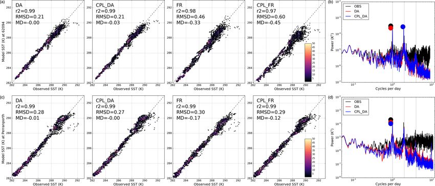
H. W. Lewis et al.: Can wave coupling improve operational regional ocean forecasts?                                            677

Figure 4. Difference in (a) mean SST (CPL_DA minus DA) due to wave coupling between experiments with data assimilation, calculated
as a 3-month seasonal mean for summer 2017; and (b) minimum instantaneous difference; (c) maximum instantaneous difference between
simulations at each grid point during the 3-month period.

Sect. 3. This is also highlighted in Fig. 5, which compares the       RMSD and MD are relatively crude summary indicators
spatial distribution of RMSD computed between the model            of model performance, in particular for assessing systems
and all observations for CPL_DA during 2017, binned in lat-        which are highly variable in space and time, and when mak-
itude and longitude areas of 0.25◦ spacing across the region       ing comparisons to a control system with relatively high skill,
where data were assimilated. Differences are negligible with       as in this study. To gain further insight into model variability,
data assimilation active (Fig. 5b), but comparing RMSD for         time series of coincident observed and simulated SST were
CPL_FR and FR suggests that the regions of greatest cooling        compared spectrally. To support spectral comparison across a
coincide with a relative degradation in RMSD, by of approx-        wide range of frequencies, the time series were initially “pre-
imately 10 %–20 % in the central North Sea and by up to a          whitened” (i.e. converted to rates of change) by computing
maximum of 50 % in the Celtic Sea (south-west approaches           the differences of successive values. A linear trend was also
to the UK, Fig. 5c).                                               removed and a split cosine taper was added to the ends of
   The comparison against in situ observations on the NWS          the detrended series in order to minimise “periodogram leak-
for each season (not shown) is more variable than Fig. 5, not-     age” (Weedon et al., 2015). The irregular spacing of the data
ing that most available sites are located near the coast (e.g.     in time required use of the Lomb–Scargle discrete Fourier
Lewis et al., 2018b). Results are improved for CPL_FR rel-         transform (Press et al., 1992) and the output periodogram
ative to FR at several locations, most notably around south-       (with 2 degrees of freedom) was smoothed using three ap-
ern and eastern UK coasts, although the general pattern is of      plications of a discrete Hanning spectral window thereby in-
wave coupling leading to poorer verification scores at many        creasing the degrees of freedom to 8.
locations.                                                            Figure 6 shows that the power spectra of the rates of
   Example comparisons between model and observations              change of SST at the CS and PP locations are in good agree-
from two locations are highlighted in Fig. 6. Given the high       ment with observed spectra for both the DA and CPL_DA
resolution of the ocean model data, and to compensate for po-      simulations (Fig. 6b, d). In particular spectral peaks at the
tential co-location errors, mean model values in a 5 × 5 grid      diurnal and semi-diurnal (M2 tide) frequencies are well rep-
cell region around each location point are compared with ob-       resented. To formally compare the time series, cross-spectral
servations, unless otherwise stated. This may lead to some         analysis was used (Weedon et al., 2015). For example, for the
smoothing of features but is considered to be more represen-       SST variability at the diurnal scale, the amplitude ratio of the
tative.                                                            rate of change of the DA simulation compared to the rate of
   The Celtic Sea observation (buoy 62094; marked as “CS”          change of the observations at the CS site is 0.87 ± 0.04 K
in Fig. 3a) is located to the south of Ireland where the influ-    (±95 % confidence interval). The phase difference at this
ence of waves on SST was shown to be seasonally varying.           frequency is 9.3 ± 5.0◦ , indicating that at the diurnal scale
The summer cooling results in greater scatter of CPL_FR            the DA simulation is approximately in phase with (i.e. not
results relative to observations for warmest temperatures          leading or lagging) the observations. Similarly, at the diur-
(Fig. 6a). Results from a nearby coastal site on the south-west    nal scale the CPL_DA simulation has an amplitude ratio of
English peninsula at Perranporth (marked “PP” in Fig. 3a)          0.77 ± 0.05 K and a phase difference of 8.0 ± 4.9◦ .
show relatively warmer simulated SST in summer (warmest               At periods shorter than the semi-diurnal scale (i.e. at
temperatures) with wave coupling in improved agreement             higher frequencies), the average power for both DA and
with observations.                                                 CPL_DA drop relative to observed at the CS and PP buoys.

www.ocean-sci.net/15/669/2019/                                                                    Ocean Sci., 15, 669–690, 2019
678 H. W. Lewis et al.: Can wave coupling improve operational regional ocean forecasts?
Figure 5. (a) Distribution of RMSD for CPL_DA during 2017 comparing simulated SST with all in situ and satellite observations prior to
assimilation. (b) Fractional change in RMSD ((CPL_DA – DA)/DA) due to wave coupling in assimilative runs. Panel (c) as (b) comparing
RMSD ((CPL – FR)/FR) due to wave coupling for non-assimilating runs. Positive differences (purple shading) indicate a relative degradation
of performance with wave coupling.
Figure 6. (a) Scatter plots comparing hourly simulated SST during 2017 from DA, CPL_DA, FR, and CPL_FR simulations with observed
values in the Celtic Sea (buoy 62094; marked CS in Fig. 3a). Summary r 2 correlation coefficient, RMSD, and MD (Model minus Observation)
statistics are listed for each model run. Shading reflects the number of points within data bins. (b) Computed power spectra (K 2 ) for observed,
DA and CPL_DA simulated SST at the Celtic Sea location. Filled circles highlight the amplitude of the peak power for each time series.
Vertical dotted lines mark diurnal, semi-diurnal, and quarter-diurnal frequencies. (c) Scatter plots comparing model and observed SST and (d)
power spectra computed for time series at the Perranporth coastal buoy (marked PP in Fig. 3a).
Additionally, a simulated quarter-daily (M4 tide) spectral 4.2 Seabed temperature (SBT)
peak is not detected in the observations. This initial assess-
ment demonstrates the utility of cross-spectral analysis as a A collection of observing sites in the German Bight provide
tool for assessing model performance and for highlighting ar- a rare source of in situ subsurface temperature observations
eas for required improved representation of high-frequency (Fig. 3a). Figure 7 compares observed seabed temperature
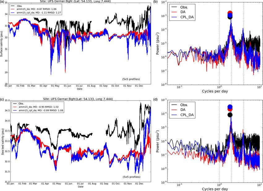
variability. (SBT) at the UFSDB (UFS Deutsche Bucht) buoy location
with simulations during 2017. Summary statistics for all sites
in the region are listed in Table 4 for comparison. In gen-
eral, results for CPL_DA and DA are very similar, with wave
coupling leading to a small degradation in RMSD and MD
Ocean Sci., 15, 669–690, 2019 www.ocean-sci.net/15/669/2019/H. W. Lewis et al.: Can wave coupling improve operational regional ocean forecasts? 679
metrics at all sites other than UFSDB. Given that the German a MLD which is typically of the order of 20–30 m deep in
Bight is a well-mixed region of the NWS, the consistency be- summer) can be seen for isolated periods of time and specifi-
tween SST and SBT impacts should be expected. For much cally during the autumn transition back to a well-mixed state.
of the year, SBT simulations at UFSDB for DA and CPL_DA Although the AMM15 ocean assimilation scheme has in-
are in good agreement with observations (correlation coeffi- troduced assimilation of temperature profiles, very few are
cient 0.98 for 2017). However, both clearly warm too quickly located in the seasonally stratified regions of the NWS (e.g.
relative to observed from mid-May, perhaps due to stronger Fig. 3 of King et al., 2018) and none were available during
mixing than observed in NEMO, and remain biased warm the 2016–2017 experiment period. It is therefore not surpris-
until early August (noting observations are unavailable from ing that assimilation of SST limits the region of tempera-
this time until mid-September). In contrast, SST results at ture differences due to wave coupling to the mixed layers
this location (not shown) are much more consistent with ob- in Fig. 8b. The impact of wave coupling on the temperature
servations throughout the year (MD of −0.03 K; Table 4). structure at and below the MLD is therefore consistent be-
It is notable that the rate of springtime seabed warming is tween the experiments with and without assimilation.
slightly reduced in CPL_DA compared to CPL, and an ob- The spatial patterns of seasonal MLD differences due to
served sharp increase in SBT in mid-June is also much better wave coupling across the NWS (Fig. 9) are most consistent
captured with wave coupling. with the pattern of SST differences between CPL_FR and FR
Power spectra of SBT at UFSDB (Fig. 7b) highlight the (Fig. 3e–h). This result also highlights that the MLD vari-
overall consistency between CPL_DA and DA, although the ability on the NWS is mostly temperature driven. The rela-
spectral peak at semi-diurnal frequency is slightly more pro- tive deepening by approximately 10 m due to wave coupling
nounced for CPL_DA. Both simulations generally underes- through the autumn transition in Fig. 8 is particularly pro-
timate the amplitude of variability relative to observations at nounced and widespread throughout the Celtic Sea and along
most frequencies. the full extent of the shelf break between Bay of Biscay to the
south to Shetland Islands in the north.
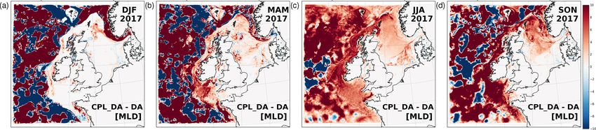
4.3 Mixed layer depth (MLD) and temperature profiles The MASSMO4 glider campaign (e.g. Palmer et al., 2018)
during spring and summer 2017 provides an independent
To better characterise and understand the impact of wave source of high vertical resolution data against which to as-
coupling in the NWS, the evolution of model temperature sess the simulated MLD results. A glider followed a west-
profiles during 2017 is considered. Figure 8 shows an exam- ward trajectory in the North Atlantic as plotted in Fig. 10a
ple of temperature differences due to wave coupling through between 21 May and 6 June 2017, crossing the shelf break
the shallow NWS depth at a location in the central North on 31 May 2017. This time of year coincides with a shal-
Sea (labelled “NS” in Fig. 3a). Results are compared both lowing mixed layer in seasonally stratified areas of the NWS
with and without ocean assimilation, and temperature pro- (e.g. Fig. 8). Figure 10a shows the simulated MLD in the re-
files are averaged daily and across a 5 × 5 collection of gion on 1 June 2016 of about 40 m on the shelf. Figure 10b
nearby grid cells. Also plotted in Fig. 8 are time series of compares the MLD recalculated from model and observation
the ocean-model-diagnosed mixed layer depth (MLD), using temperature and salinity data, based on Kara et al. (2000)
the density-based definition of Kara et al. (2000). The an- from vertical profiles measured by the glider. There is consid-
nual variation in MLD illustrates that the selected location erable variability in MLD during the observed period, which
is seasonally stratified – well mixed during winter and transi- is captured relatively well by all simulations (RMSD of about
tioning to being stratified below a shallow mixed layer during 9 m). On average, the uncoupled FR and DA results are bi-
summer (e.g. Huthnance et al., 2009). ased too shallow (by 2.9 m for FR and 2.2 m for DA) while
In summer there is a clear dipole in the structure of temper- the deepening due to wave coupling results in a smaller MLD
ature differences with relative cooling due to waves through difference, although now biased deep (by 0.9 m for CPL_FR
the shallow mixed layer and warming at depth (Fig. 8b, c). and 1.7 m for CPL_DA). Periods when coupled MLD values
The intervening layer within 10 m below the MLD shows were deeper than observations occur during late May, when
large temperature differences (> 1 K). This structure is con- the glider was located on the NWS. In June, when the glider
sistent with a mechanism of enhanced mixing due to a net in- was off-shelf and simulation errors are increased, the impact
put of momentum from surface waves (Fig. 1b, e), deepening of wave coupling leads to clearer improvement relative to un-
the MLD, thickening the pycnocline, and encouraging mix- coupled simulations.
ing of warmer near-surface water further from the surface. This analysis has demonstrated an annually varying cycle
A deepening MLD in summer also implies that surface heat- in the impact of wave coupling on ocean temperatures on
ing is warming a larger volume of water with wave coupling, the NWS, associated with a deepening of the mixed layer
thereby leading to a relatively cooler mixed layer and SST through enhanced mixing. It is encouraging that the quanti-
(Fig. 3). The model-diagnosed MLD is typically deepened tative agreement between model results and observations is
by a few metres between simulations with and without wave not degraded considerably, and improves in some respects. In
coupling in summer. However, differences of up to 10 m (for practice, the ocean model physics (e.g. turbulence and radia-
www.ocean-sci.net/15/669/2019/ Ocean Sci., 15, 669–690, 2019680 H. W. Lewis et al.: Can wave coupling improve operational regional ocean forecasts?
Figure 7. (a) Time series of simulated seabed temperature (SBT) during 2017 from DA and CPL_DA simulations and observed values in
the German Bight (buoy UFSDB). Summary MD and RMSD statistics are listed for each run. (b) Computed power spectra for observed, DA
and CPL_DA simulated SBT. Filled circles highlight the amplitude of the peak power for each time series. Vertical dotted lines mark diurnal,
semi-diurnal, and quarter-diurnal frequencies.
Table 4. Summary statistics comparing DA and CPL_DA results for sea surface temperature (SST) and seabed temperature (SBT) with
co-located observations during 2017 at sites in the German Bight (starred symbols in Fig. 3a).
Mean difference (MD) (Model minus Obs.) RMSD
FINO1 FINO3 NsbII TWEMS UFSDB FINO1 FINO3 NsbII TWEMS UFSDB
SST (K)
DA 0.06 0.04 −0.12 −0.02 −0.01 0.21 0.37 0.24 0.25 0.48
CPL_DA 0.03 0.02 −0.12 −0.02 −0.03 0.23 0.39 0.24 0.25 0.49
SBT (K)
DA 0.03 0.24 0.14 0.00 0.33 0.20 0.59 0.47 0.16 0.75
CPL_DA 0.06 0.27 0.20 0.02 0.30 0.22 0.67 0.55 0.17 0.67
tion schemes) and assimilation options are developed to pro- NWS in all seasons of up to 1 psu along the Bay of Bis-
vide forecast systems which best match the available obser- cay and German Bight coasts, but more typically less than
vations. To date, these have been developed in a forced-mode 0.3 psu across the North Sea, English Channel, and some
ocean-only context. Having established an effective baseline western UK coastal areas. This suggests that the effect of
wave-coupled configuration for the NWS, it is clear that fur- river freshening is diminished, perhaps through a combina-
ther improvements can be realised through revisiting param- tion of enhanced vertical mixing or lateral advection. By con-
eter choices within these schemes. trast, wave coupling leads to reduced SSS at the outflow from
the Bristol Channel and northward through the Irish Sea.
4.4 Salinity Schloen et al. (2017) studied the impact of wave coupling
on salinity in the southern North Sea in detail using ocean
The impact of wave coupling on the NWS sea surface salin- and wave models with unstructured grids based on a month-
ity (SSS) during 2017 is summarised by the mean differences long simulation, and described how wave-induced transport
between CPL_DA and DA in Fig. 11a. To first-order approx- of salt led to changes in the horizontal salinity distribution
imation these results are independent of whether ocean data in the vicinity of the German Wadden Sea islands. There is
assimilation was active, so CPL_FR and FR results are omit- remarkably strong agreement between Fig. 11b and the re-
ted. There is also no clear variation in the impact of waves sults of Schloen et al. (2017; Fig. 10a) in the distribution of
across the different seasons. fresher and saltier surface water due to wave coupling over a
As expected, the greatest sensitivity of salinity to wave broader area along the Dutch and German coasts. Both this
coupling is focused on areas where river freshwater mixes study and their results show saltier water north and south-
into the ocean. The net tendency is for increased SSS across
Ocean Sci., 15, 669–690, 2019 www.ocean-sci.net/15/669/2019/H. W. Lewis et al.: Can wave coupling improve operational regional ocean forecasts? 681 Figure 8. Evolution of daily mean temperature profiles through 2017 at a central North Sea location (see Fig. 3a). Temperature differences due to wave coupling are shown in (b) between CPL_DA and DA and in (c) for CPL_FR and FR. The lines plotted show MLD for simulations without wave coupling in black and with wave coupling in green. Figure 9. Seasonal mean differences in simulated mixed layer depth (MLD) in CPL_DA relative to DA during 2017. ward of the Wadden Sea islands (fed from the river Ems), tributed to the use of a climatological freshwater boundary and larger increases in salinity along the Danish coast fo- condition in the operational AMM15 configuration consid- cused near the outflow of the Elbe. Immediately to the west, ered in this study. However, there is also a clear impact of a dipole of salinity differences occurs at the outflow from the wave coupling on the salinity variability throughout 2017. Weser, which leads to relatively fresher water propagating CPL_DA results show greater variability across the year at further off-shore into the North Sea. Finally, the impact of both levels, with good correspondence to the observed vari- wave coupling in a relatively constrained area near the Rhine ability which is not reflected in the summary MD and RMSD outflow towards the south in Fig. 11b is characterised by a metrics. This is demonstrated further by the agreement be- relative freshening, again in good agreement with Schloen et tween power spectra for the observed and simulated time se- al. (2017). Apart from some near-coastal differences along ries in Fig. 12b and d. Both simulations reproduce the ob- eastern England, the distribution of mean seabed salinity served peak at the semi-diurnal M2 tidal frequency (12.42 h) (SBS) differences (Fig. 11c) in the region is highly consis- well, with limited impact of wave coupling evident. The re- tent with the SSS results. This implies that wave-induced sults are also consistent at this site for higher frequencies, changes to horizontal rather than vertical mixing processes with further spectral peaks in surface salinity corresponding are dominant. Summary statistics comparing model simula- to the M4 and M6 tidal components. While these spectral tions during 2017 with observed SSS and SBS are listed in peaks are maintained in the salinity simulations at the seabed, Table 5. they are not observed. This might suggest that accounting for Results in Table 5 reflect the larger sensitivity to wave ef- the effects of seabed–wave coupling in shallow seas could fects for the three locations closer to the coast, for which lead to further improvement (e.g. Soulsby et al., 1995). Al- summary metrics for both SSS and SBS are markedly im- ternatively, this difference in observations could be related proved with wave coupling at FINO1 (yellow star) and to how freshwater flux boundary conditions are distributed TWEMS (dark blue), both located in the area of increased vertically in NEMO. There is also a clear difference in the SSS, while results are degraded at UFSDB in the region of variance in CPL_DA and DA at periods longer than daily, freshening salinity (light blue; Fig. 11). especially for SBS (Fig. 12d). CPL_DA shows improved re- Figure 12 shows a comparison between CPL_DA and DA sults compared to DA relative to the observed spectrum. This simulations with observed SSS and SBS through 2017 at is consistent with the more qualitative assessment of longer- UFSDB. Both CPL_DA and DA are clearly too fresh with term variability in Fig. 12c. substantial biases in SSS and SBS. This can be partly at- www.ocean-sci.net/15/669/2019/ Ocean Sci., 15, 669–690, 2019
682                                     H. W. Lewis et al.: Can wave coupling improve operational regional ocean forecasts?

Figure 10. (a) Daily mean MLD on 1 June 2017 simulated by FR for a section of the model domain to the north of Scotland. Contours mark
the model bathymetry in 50 m intervals and the thick black line marks the glider trajectory. (b) MLD calculated from observed and model
profiles following the glider trajectory over the observation period. Grey shading indicates the mixed layer according to glider observations.

Figure 11. (a) Annual mean differences in simulated sea surface salinity (SSS) in CPL_DA relative to DA during 2017. (b) Zoom of annual
mean SSS differences across the southern North Sea; and (c) differences in annual mean seabed salinity (SBS) in this region. The location of
observing sites in the German Bight referenced in the text are shown (see also Fig. 3a).

   Results from the nearby TWEMS buoy, located on the                    4.5    Sea surface height (SSH)
edge of the region of increased salinity in Fig. 11b (dark blue
marker in Figs. 3a and 11), are shown in Fig. 13. The in-
                                                                         The summary statistics presented in Sect. 3 indicate that the
creased salinity at TWEMS reduces the negative bias against
                                                                         net impact of wave processes on sea surface height (SSH) is
observations. Power spectra from the 2017 results in Fig. 13b
                                                                         negligible in terms of long-term statistics for the simulated
and d highlight a much greater amplitude of the salinity semi-
                                                                         sea level anomaly (SLA) in comparison with satellite altime-
diurnal cycle at both the surface and seabed in the DA simu-
                                                                         ter observations. The spatial distribution of RMSD for each
lation than in observations, which is improved for CPL_DA
                                                                         experiment (not shown) indicates generally neutral changes
results. Focusing on the time series of SSS and SBS during
                                                                         across much of the NWS but improvements of approximately
January 2017 only (Fig. 13a and c) demonstrates a remark-
                                                                         10 % across the North Sea with wave coupling.
able improvement of the agreement between observed and
                                                                            Of more relevance for natural hazard prediction are the
simulated salinity at both the surface and seabed with the
                                                                         extremes of simulated SSH, given the requirement of ac-
inclusion of wave processes. This change of amplitude sug-
                                                                         curate SSH simulation for warnings of coastal storm surge
gests the influence of wave coupling in modulating wave–
                                                                         and inundation. Figure 14 therefore shows the distribution
tide interactions in the region (e.g. Lewis et al., 2019), but
                                                                         of the largest positive and negative SSH differences between
a more systematic study is beyond the scope of the current
                                                                         CPL_DA and DA during winter 2016/2017, noting these dif-
work.
                                                                         ferences are independent of whether ocean data assimilation
                                                                         was active or not. Greatest variability occurs during winter
                                                                         and autumn seasons, focused around coastlines as might be
                                                                         expected. Instantaneous SSH reductions of up to 10 cm can

Ocean Sci., 15, 669–690, 2019                                                                           www.ocean-sci.net/15/669/2019/
You can also read