Reproducing pyroclastic density current deposits of the 79 CE eruption of the Somma-Vesuvius volcano using the box-model approach - Solid Earth
←
→
Page content transcription
If your browser does not render page correctly, please read the page content below
Solid Earth, 12, 119–139, 2021
https://doi.org/10.5194/se-12-119-2021
© Author(s) 2021. This work is distributed under
the Creative Commons Attribution 4.0 License.

Reproducing pyroclastic density current deposits of
the 79 CE eruption of the Somma–Vesuvius volcano
using the box-model approach
Alessandro Tadini1,2,3 , Andrea Bevilacqua2 , Augusto Neri2 , Raffaello Cioni3 , Giovanni Biagioli2,4 ,
Mattia de’Michieli Vitturi2 , and Tomaso Esposti Ongaro2
1 Laboratoire  Magmas et Volcans, Université Clermont Auvergne, CNRS, IRD, OPGC,
6 Avenue Blaise Pascal, 63178 Aubière, France
2 Istituto Nazionale di Geofisica e Vulcanologia, Sezione di Pisa, Via Cesare Battisti 53, 56125 Pisa, Italy
3 Dipartimento di Scienze della Terra, Università di Firenze, Via G. La Pira 4, 50121 Firenze, Italy
4 Dipartimento di Matematica e Geoscienze, Università degli Studi di Trieste, Via Weiss 2, 34128 Trieste, Italy

Correspondence: Alessandro Tadini (alessandro.tadini@uca.fr)

Received: 10 August 2020 – Discussion started: 9 October 2020
Revised: 23 November 2020 – Accepted: 2 December 2020 – Published: 20 January 2021

Abstract. We use PyBox, a new numerical implementation               the performance of the PyBox code. The study findings sug-
of the box-model approach, to reproduce pyroclastic den-             gest that the simplified box-model approach has promise for
sity current (PDC) deposits from the Somma–Vesuvius vol-             applications in constraining the plausible range of the input
cano (Italy). Our simplified model assumes inertial flow front       parameters of more computationally expensive models. This
dynamics and mass deposition equations and axisymmetric              could be done due to the relatively fast computational time of
conditions inside circular sectors. Tephra volume and density        the PyBox code, which allows the exploration of the physical
and total grain size distribution of EU3pf and EU4b/c, two           space of the input parameters.
well-studied PDC units from different phases of the 79 CE
Pompeii eruption, are used as input parameters. Such units
correspond to the deposits from variably dilute, turbulent
PDCs. We perform a quantitative comparison and uncertainty           1   Introduction
quantification of numerical model outputs with respect to the
observed data of unit thickness, inundation areas and grain          The increased availability of numerical models capable of
size distribution as a function of the radial distance to the        reproducing, with various degrees of simplification, the dy-
source. The simulations consider (i) polydisperse conditions,        namics of pyroclastic flows (see Sulpizio et al., 2014, for a
given by the total grain size distribution of the deposit, or        review) provided geoscientists and civil authorities with new
monodisperse conditions, given by the mean Sauter diameter           valuable tools for better understanding natural phenomena
of the deposit; (ii) axisymmetric collapses either covering the      and for more accurate hazard assessments. Several modelling
whole 360◦ (round angle) or divided into two circular sec-           approaches have been developed over the past years for py-
tors. We obtain a range of plausible initial volume concen-          roclastic density currents (PDCs), from simplified 1D kinetic
trations of solid particles from 2.5 % to 6 %, depending on          models (Malin and Sheridan, 1982; Sheridan and Malin,
the unit and the circular sector. Optimal modelling results of       1983; Dade and Huppert, 1995b, 1996; Bursik and Woods,
flow extent and deposit thickness are reached on the EU4b/c          1996; Doyle et al., 2010; Esposti Ongaro et al., 2016; Fauria
unit in a polydisperse and sectorialized situation, indicating       et al., 2016) up to more complex, 2D depth-averaged models
that using total grain size distribution and particle densities as   (Patra et al., 2005, 2020; Charbonnier and Gertisser, 2009;
close as possible to the real conditions significantly improves      Kelfoun et al., 2009, 2017; Tierz et al., 2018; de’Michieli
                                                                     Vitturi et al., 2019) and computationally expensive but phys-

Published by Copernicus Publications on behalf of the European Geosciences Union.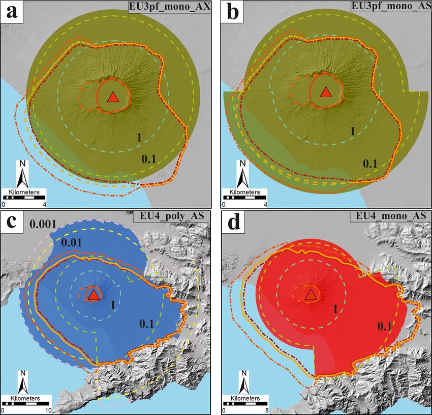
120                                 A. Tadini et al.: Reproducing pyroclastic density current deposits of the 79 CE eruption

ically realistic 2D (axisymmetric) and 3D models (Esposti             parameters (especially thickness and grain sizes), which al-
Ongaro et al., 2002, 2007, 2012, 2019; Todesco et al., 2002,          lows a further investigation of the strengths and limitations
2006; Neri et al., 2003; Dufek and Bergantz, 2007; Dufek et           of the PyBox model when used to simulate different PDC
al., 2015; Dufek, 2016).                                              types.
    Although the 1D kinetic approaches cannot capture the
multidimensional features of dynamics, they represent an im-
portant tool for several purposes. Firstly, it is practical to rely   2     Numerical model and data sources
on simplified and fast numerical codes, which can be run
104 –106 times without an excessive computational expense,            2.1    The box-model approach and the PyBox code
in order to produce statistically robust probabilistic hazard
maps (Neri et al., 2015; Bevilacqua et al., 2017; Aravena et          PyBox is a numerical implementation of the box-model
al., 2020). Furthermore, since 2D or 3D multiphase models             integral formulation for axisymmetric gravity-driven parti-
require high computational times, often on the order of days          cle currents based on the pioneering work of Huppert and
or weeks for a single simulation, it is convenient to use sim-        Simpson (1980). The theory is detailed in Bonnecaze et al.
plified approaches, such as the box model, in order to con-           (1995) and Hallworth et al. (1998). The volume extent of
strain the input space (Ogburn and Calder, 2017; Bevilacqua           gravity currents is approximated by an ideal geometric el-
et al., 2019a). Finally, extensively testing the numerical mod-       ement, called “box”, which preserves its volume and geo-
els in a statistical framework and evaluating the difference          metric shape class and only changes its height/base ratio
between model outputs and actual observations also allows             through time (Fig. 1). The box does not rotate or shear but
estimation of the effect of the various modelling assump-             only stretches out as the flow progresses. In this study the
tions under uncertain input conditions (e.g. Patra et al., 2018,      geometric shape of the box is assumed to be a cylinder; i.e.
2020; Bevilacqua et al., 2019b). Model uncertainty is proba-          we assume axisymmetric conditions.
bly the most difficult class of epistemic uncertainty to evalu-          The model describes the propagation of a turbulent
ate robustly, but it is indeed a potentially large component of       particle-laden gravity current, i.e. a homogeneous fluid with
the total uncertainty affecting PDC inundation forecasts.             suspended particles. Inertial effects are assumed to dominate
    In this paper, we test the suitability of the box-model ap-       with respect to viscous forces and particle–particle interac-
proach, as implemented numerically in the PyBox code (Bi-             tions. Particle sedimentation is modelled and modifies the
agioli et al., 2019), by quantifying its performance when re-         current inertia during propagation. In this study we assume
producing some key features of the well-characterized PDC             the classical dam break configuration, in which a column of
deposits from one of the best studied and documented vol-             fluid instantaneously collapses and propagates, under grav-
canic events: the 79 CE eruption of the Somma–Vesuvius                ity, in a surrounding atmosphere with uniform density ρatm .
(SV) volcano. The box model is able to describe the main              Other authors (Bonnecaze et al., 1995; Dade and Huppert,
features of large-volume (VEI 6 to 8; Newhall and Self,               1995a, b, 1996) have instead considered gravity currents pro-
1982), low-aspect-ratio ignimbrites, whose dynamics are               duced by the constant flux release of dense suspension from a
dominantly inertial (Dade and Huppert, 1996; Giordano and             source. Our approach does not assume constant stress acting
Doronzo, 2017), although there was some debate on the                 on the basal area as in Dade and Huppert (1998). Constant
mechanism of flow emplacement in that case study (Dade                stress dynamics have been explored in literature, and they
and Huppert, 1997; Wilson, 1997). In general, thick den-              can lead to different equations if the basal area grows lin-
sity currents are able to propagate inertially even on flat to-       early or with the square of the radius (Kelfoun et al., 2009;
pographies, and the effect of friction is usually negligible.         Kelfoun, 2011; Ogburn and Calder, 2017; Aspinall et al.,
Low-aspect-ratio ignimbrites or flows produced can gener-             2019). Bevilacqua (2019) provides a brief derivation of var-
ally be modelled as “inertial PDCs” for most of their run-out         ious examples of box-model equations either under constant
(de’Michieli Vitturi et al., 2019). However, the model has            stress or sedimentation.
never been tested against PDC generated by VEI 5 Plinian                 Our model consists of a set of ordinary differential equa-
eruptions (Shea et al., 2011). The procedure involves the cal-        tions, which provide the time evolution of flow front distance
culation of the difference between model output and field             from the source, l(t), together with the current height h(t)
data in terms of (i) thickness profile, (ii) areal invasion over-     and the solid particle volume fraction (εi )i=1,...,N , N being
lapping and (iii) grain size (GS) volume fractions at various         the number of particle classes considered. The volume frac-
distances from the source (see, for example, Dade and Hup-            tions refer to a constant volume of the mixture flow, not re-
pert, 1996; Kelfoun, 2011; Charbonnier et al., 2015). Tierz           duced by the deposition.
et al. (2016a, b) and Sandri et al. (2018) proposed a quan-              PDCs are driven by their density excess with respect to
tification of the uncertainty derived from the energy cone ap-        the surrounding air: the density of the current ρc is defined as
proach that relies on the comparison between invaded area             the sum of the density of an interstitial gas, ρg and the bulk
and maximum run-out of model output and field data. Our               densities of the pyroclasts carried by the flow, (ρis )i=1,...,N .
approach aims at the more detailed comparison of physical             In this study we assume ρatm 6 = ρg i.e. the interstitial gas is

Solid Earth, 12, 119–139, 2021                                                             https://doi.org/10.5194/se-12-119-2021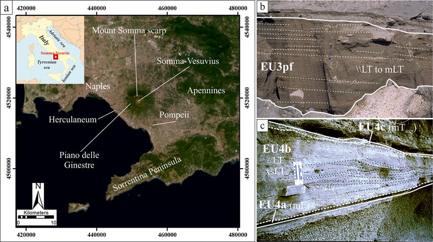
A. Tadini et al.: Reproducing pyroclastic density current deposits of the 79 CE eruption                                                121

Figure 1. (a) Schematic diagram of an inertial gravity current with a depth hc , flow front velocity uc and density ρc in an ambient fluid of
density ρ0 (modified from Roche et al., 2013); (b) evolution of channelized currents through a series of equal-area rectangles, according to
the model (hence the name “box model”).

hotter than surrounding atmosphere, differently from Neri                class is the ratio of the ith deposited mass to the ith solid
et al. (2015) and Bevilacqua et al. (2017). The code allows              density multiplied by the packing fraction α measured in the
ρatm > ρg , but thermal properties remain constant for the du-           deposit. More details on the numerical solver are provided in
ration of the flow. A proper way to express the density con-             Appendix A.
trast between the current and the ambient fluid is given by                 In the calculation of the region invaded by a PDC, first
the reduced gravity g 0 , which can be rewritten in terms of the         we calculate the maximum flow run-out over flat ground, i.e.
densities and the volume fractions described above (see Bia-             the distance at which ρc = ρatm . The flow stops propagating
gioli et al., 2019). That said, we make some additional sim-             when the solid fraction becomes lower than a critical value,
plifications. First, we assume that the mixture flow regime              and, although not modelled, in nature the remaining mixture
is incompressible and inviscid, since we assume that the dy-             of gas and particles lifts off, possibly generating a phoenix
namics of the current are dominated by the balance between               cloud if hot gas is assumed. In the case of monodisperse
inertial and buoyancy forces. The assumption of incompress-              systems there are analytical solutions for the maximum flow
ibility implies that the initial volume V0 remains constant.             run-out (Bonnecaze et al., 1995; Esposti Ongaro et al., 2016;
Moreover, we assume that, within the current, turbulent mix-             Bevilacqua, 2019). Then, once a vent location is set, we as-
ing produces a vertically uniform distribution of particles.             sess the capability of topographic reliefs to block the current.
The particles are assumed to sediment out of the current at              In particular, the invasion areas are obtained by using the so-
a rate proportional to their constant terminal (or settling) ve-         called energy-conoid model, based on the assumption of non-
locity (wis )i=1,...,N and, once deposited, they cannot be re-           linear, monotonic decay of flow kinetic energy with distance
entrained by the flow; the converse was explored in Fauria               (Neri et al., 2015; Bevilacqua, 2016; Esposti Ongaro et al.,
et al. (2016). Finally, surface effects of the ambient fluid are         2016; Bevilacqua et al., 2017; Aspinall et al., 2019; Aravena
neglected.                                                               et al., 2020). In more detail, we compare the kinetic energy
   Under these hypotheses, the box model for particle-laden              of the current front and the potential energy associated with
gravity currents states that the velocity of the current front (u)       the obstacles encountered. In this approach we are neglect-
is related to the average depth of the current (h) by the von            ing returning waves. When investigating the current flow on
                                                       1                complex topographies, we finally consider that the flow may
Kármán equation for density currents u = Fr g 0 h 2 , where
Fr is the Froude number, a dimensionless ratio between in-               start from positive elevation or encounter upward slopes af-
ertial and buoyancy forces (Benjamin, 1968; Huppert and                  ter downward slopes. In this case, we compare the kinetic
Simpson, 1980) and g 0 is the reduced gravity. In addition, we           energy at a given distance from the vent and the difference in
assume that particles can settle to the ground and this process          level experienced by the current with respect to the minimum
changes the solid particle fractions (εi )i=1,...,N .                    elevation previously run into.
   The box model for axisymmetric currents thus reads                       In the PyBox code, the main input parameters are summa-
                                                                         rized by (a) the total collapsing volume (expressed in terms
 dl               1                                                     of the dimension of the initial cylinder or rectangle with
     = Fr g 0 h 2 ,                                        (1)
dt                                                                       height = h0 and radius/base = l0 ); (b) the initial concentra-
l 2 h = l02 h0 ,                                           (2)           tion of solid particles, subdivided (for polydisperse simula-
d (εi ) wi εi   s                                                        tions) into single particle volumetric fractions (ε0 ), with re-
        =            ∀i = 1, . . ., N.                     (3)           spect to the gas; (c) the density of single particles ρs ; (d)
    dt         h
                                                                         ambient air density (ρatm = 1.12 kg m−3 ) and gravity cur-
By solving these equations, we computed the amount of mass               rent temperature; (e) Froude number of the flow, experimen-
loss by sedimentation, per unit area and per time step, for              tally measured by Esposti Ongaro et al. (2016) as Fr = 1.18;
each particle class. The thickness profile of the ith particle

https://doi.org/10.5194/se-12-119-2021                                                                  Solid Earth, 12, 119–139, 2021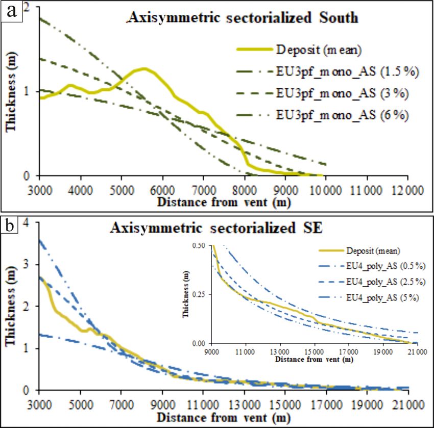
122                                 A. Tadini et al.: Reproducing pyroclastic density current deposits of the 79 CE eruption

and (f) gravity acceleration (g = 9.81 m s−2 ). With respect to      complications, since it actually presents a second fallout bed
points (b) and (c), more details are provided in Sect. 3.2.          (EU4a2) interlayered within the level EU4b. This fallout bed
                                                                     can be clearly recognized only in distal sections of the south-
2.2   The EU3pf and EU4b/c units from the 79 CE                      ern sector, while in the north and in the west it is represented
      eruption of SV                                                 by a discontinuous horizon of ballistic ejecta. Level EU4a2
                                                                     divides level EU4b into two parts, which are approximately
The 79 CE eruption of SV volcano (Fig. 2a) involved a com-           two-thirds (the lower one) and one-third (the upper one) of
plex sequence of fallout and PDC phases, resulting in the            the total thickness of level EU4b (Gurioli, 1999). Run-out of
deposition of a sequence of eruptive units (EUs; Cioni et al.,       the EU4b PDC is one of the largest run-outs observed for
1992). The EU3pf and EU4b/c units (Fig. 2b) represent the            the SV PDCs; to the south it was deposited up to ≈ 20 km
two main PDC deposits, which have been traced over a large           from vent area (Gurioli et al., 2010). This unit has been ex-
area around the volcano and characterized for their most rel-        tensively studied by Gurioli (1999), who highlighted that the
evant physical parameters (Gurioli et al., 2010; Cioni et al.,       high shear rate exerted by the EU4b is clearly evidenced by
2020).                                                               the formation of traction carpet bedding and local erosion of
   The EU3pf unit records the phase of total column collapse         the pumice-bearing layer of the underlying EU4a. The EU4b
closing the Plinian phase of the eruption. This is ca. 1 m thick     deposit can be interpreted as being derived from a short-
on average, radially dispersed up to 10 km from the vent area        lived sustained, unsteady, density-stratified current. From a
and moderately controlled by local topography. The variabil-         sedimentological point of view, EU4b shows clear vertical
ity of vertical and lateral facies (Gurioli, 1999; Gurioli et al.,   grain size and textural variations, from cross-bedded, fine-
1999) are probably related to local variation in turbulence,         lapilli to coarse-ash laminae at the base up to a massive, fine-
concentration and stratification of the current. Median clast        ash-bearing, poorly sorted, matrix-supported bed at the top
size gradually decreases from proximal to distal locations,          (Gurioli, 1999). During deposition of EU4b, ash elutriated
and the coarsest deposits, generally present as breccia lenses       from the current formed a convective plume dispersed from
in the EU3pf sequence, are located within paleo-depressions.         the prevailing winds in a south-eastern direction, which de-
Gurioli et al. (1999) showed that the deposits reflect differ-       posited EU4c mainly by fallout. The clear field association of
ent topographic situations in different sectors around the vol-      these two deposits (indicated as EU4b/c) gives here the un-
cano. South of SV the relatively smooth paleo-topography             common possibility to evaluate with a larger accuracy two of
only locally affected the overall deposition of this PDC. In         the most important PDC source parameters: erupted volume
the eastern sector of SV, the interaction of the current with        and total grain size distribution (TGSD).
the ridge representing the remnants of the old Mount Somma
caldera (Fig. 2a) possibly triggered a general increase in the
current turbulence and velocity and a more efficient air inges-
tion, which resulted in the local deposition of a thinly strati-     3     Methods
fied sequence. To the west of SV, the presence of a breach in
the caldera wall and of an important break in slope in the area      3.1    Model input parameters and field data for
of Piano delle Ginestre (Fig. 2a), possibly increased deposi-               comparison
tion from the PDC, producing a large, several metres thick
depositional fan toward the sea-facing sectors (like in Hercu-       The main properties of the EU3pf and EU4b/c units – thick-
laneum; Fig. 2a). In the northern sector of SV, the deeply           nesses, total volume, maximum run-out and TGSD – have
eroded paleo-topography, with many radial valleys cut on             been calculated in Cioni et al. (2020) and partially processed
steep slopes, favoured the development within the whole cur-         to fit with PyBox input requirements. Densities of single
rent of a fast-moving, dense basal underflow able to segregate       grain sizes and emplacement temperatures of PDCs (T =
the coarse, lithic material and to deposit thick lobes in the        600 K for both EU3pf and EU4) are derived from Barberi et
main valleys and of a slower and more dilute portion travel-         al. (1989) and Cioni et al. (2004). Total volume, TGSD, den-
ling and depositing thin, stratified beds also on morphologi-        sities and temperature obtained from field data are used as the
cal highs.                                                           main inputs of PyBox. The model produces several outputs:
   EU4 records a subsequent phase of the eruption and was            (i) mean unit thickness as a function of the radial distance
related by Cioni et al. (1999) to the onset of the caldera           from the source, (ii) inundated area and (iii) grain size dis-
collapse. This complex unit has been subdivided into three           tribution as a function of radial distance from the source. All
distinct layers (Cioni et al., 1992): a thin basal fallout layer     these outputs are finally compared to the corresponding field
(EU4a), a PDC deposit derived from the collapse of the short-        data. The initial volumetric fraction ε0 of the solid particles
lived column that emplaced the EU4a layer (EU4b), and the            over the gas is the main tuning parameter that is explored to
products of the co-ignimbritic plume mainly derived by ash           fit the outputs with the field data. This procedure is repeated
elutriation from the current that deposited EU4b (EU4c).             under monodisperse and polydisperse conditions and by per-
Gurioli (1999) illustrates how the EU4 unit has additional           forming round-angle axisymmetric collapses or sectorialized

Solid Earth, 12, 119–139, 2021                                                            https://doi.org/10.5194/se-12-119-2021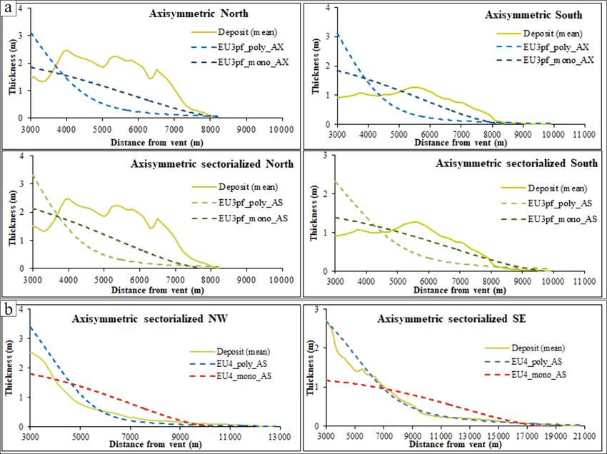
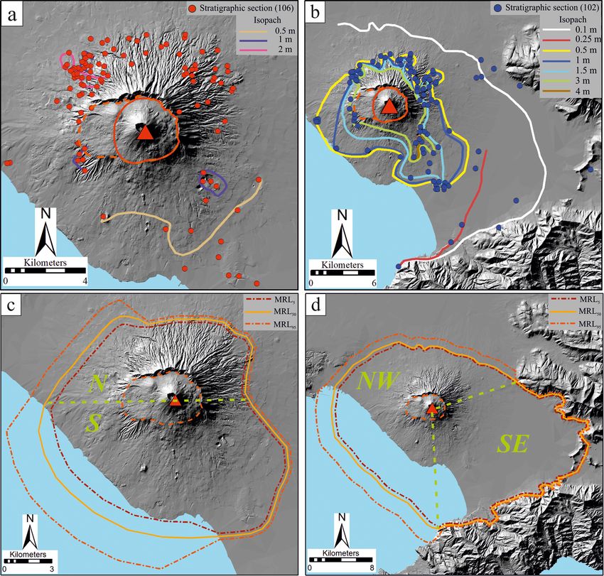
A. Tadini et al.: Reproducing pyroclastic density current deposits of the 79 CE eruption                                                   123

Figure 2. (a) Location of the Somma–Vesuvius volcano. Coordinates are expressed in the UTM WGS84-33N system. (b) The EU3pf unit
(Cioni et al., 2020); (c) the EU4 unit (Cioni et al., 2020). In (b), solid lines are the limits between EUs, dashed lines are the limits between
levels (a, b and c) and dotted lines are lithofacies stratifications. Lithofacies terminology is derived from Branney and Kokelaar (2002): //LT
– “plane-parallel lapilli tuff”; mLT – “massive lapilli tuff”; xsLT – “cross-stratified lapilli tuff”; mL – “massive lapillistone”; and mTaccr –
“massive tuff with accretionary lapilli”. Service layer credit source: Esri, DigitalGlobe, GeoEye, Earthstar Geographics, CNES/Airbus DS,
USDA, USGS, AeroGRID, IGN and the GIS User Community

collapses, i.e. divided into two circular sectors with different          display the different sectors for both EU3pf and EU4b/c for
input parameters.                                                         which different volumes have been calculated.

3.1.1   Thickness, maximum run-out and volumes                            3.1.2    Density data

Cioni et al. (2020) recently revised and elaborated on a large            In order to provide density values for each GS, we used the
amount of field data from EU3pf and EU4b/c (106 and 102                   mass fractions of the different components (juveniles, lithics
stratigraphic sections, respectively), tracing detailed isopach           and crystals – see Table S1 in the Supplement) calculated by
maps (Fig. 3a and b) and defining the maximum run-out                     Gurioli (1999). Such values were associated with the aver-
distance (the ideal 0 m isopach) and the related uncertainty.             aged density measurements for these three components pre-
Given the objective difficulty in tracing the exact position              sented in Barberi et al. (1989), through which we extrapo-
of a 0 m isopach for the deposit of a past eruption, Cioni                lated the weighted mean (with respect to mass fraction) den-
et al. (2020) proposed to define three different outlines of              sity of each grain size class for both EU3pf and EU4b/c units
PDC maximum run-outs, namely the “5th percentile”, “50th                  (Table 2).
percentile” and “95th percentile” (called maximum run-out
lines, MRLs), based on the uncertainty associated with each               3.1.3    Grain size data: total grain size distribution and
segment of the proposed 0 m isopach. The MRLs of EU3pf                             mean Sauter diameter (MSD)
and EU4b are shown in Fig. 3c and d, respectively.
   Cioni et al. (2020) also calculated the volumes of both                The TGSD estimations are necessary to do simulations under
EU3pf and EU4b/c, using these maps to derive a digital el-                polydisperse conditions. The present version of PyBox takes
evation model of the deposits with the triangular irregular               as input the volumetric TGSD (i.e. in terms of volumetric
network (TIN) method (Lee and Schachter, 1980). In this                   percentages), while TGSD data from Cioni et al. (2020) are
study, we considered volume estimations (Table 1) related                 in weight percentages. These latter values have been there-
to the MRL50 , the 50th percentile of the maximum run-out                 fore converted into volumetric percentages by considering
distance.                                                                 the above-mentioned densities (Table 2). Figure 4 displays
   Given the asymmetric shape of unit EU4b/c and, partially,              the volumetric TGSDs employed for EU3pf (total, N and S)
of unit EU3pf, we have also calculated the volumes dividing               and the EU4b/c (total, NW and SE).
each unit into two circular sectors: N and S for EU3pf; NW                   In the simulations under monodisperse conditions, we
and SE for EU4b/c. These subdivisions have also been used                 used the value of mean Sauter diameter (MSD) of the vol-
to calculate the related TGSDs (see Sect. 3.1.3) and to per-              umetric TGSD (e.g. Neri et al., 2015). According to Fan and
form sectorialized simulations (see Sect. 4). Figure 3c and d             Zhu (1998), the Sauter diameter of each particle class size is

https://doi.org/10.5194/se-12-119-2021                                                                     Solid Earth, 12, 119–139, 2021
124 A. Tadini et al.: Reproducing pyroclastic density current deposits of the 79 CE eruption
Figure 3. Thicknesses and isopach lines for the (a) EU3pf and (b) EU4b/c units; MRLs of the (c) EU3pf and (d) EU4b/c units. Inferred
position of 79 CE vent (red triangle) and SV caldera outline (dark orange dashed line) after Tadini et al. (2017). Light green dashed lines
delimit the sectors (N–S for EU3pf and NW–SE for EU4) of the different column collapses. Background DEM from Tarquini et al. (2007).
Table 1. Volume of the EU3pf and EU4b/c units.
Unit EU3pf EU4b/c
Sector Total N S Total NW SE
Volume (km3 ) 0.188 0.096 0.092 0.331 0.180 0.151
also called d32 (see also Breard et al., 2018), and it is the di- where Vi is the cumulative volume of the ith grain size class,
ameter of a sphere having the same ratio of external surface and ri is the radius of the ith grain size. The mean MSD is
to volume as the particle, which is given by finally derived as
6V d3
d32 = = v2 , (4)
N
S ds
P
ni di3
i=1
where V is the particle volume, S is the particle surface, dv
MSD (8) = −log2 , (6)
is the diameter of a sphere having the same volume as the N
P
nj dj2
particle and ds is the diameter of a sphere having the same j =1
external surface as the particle. In order to obtain a value
for the MSD instead, given a deposit sample divided into N where di and dj are the diameters of, respectively, the ith and
grain size classes, we have initially calculated the number of j th grain sizes.
particles of each grain size i = 1, . . ., N , that is Table 3 summarizes the calculated MSDs for the studied
Vi units (in 8), along with the corresponding density values (ob-
ni = 4 3 , (5)
3 π ri
tained interpolating those in Table 2).
Solid Earth, 12, 119–139, 2021 https://doi.org/10.5194/se-12-119-2021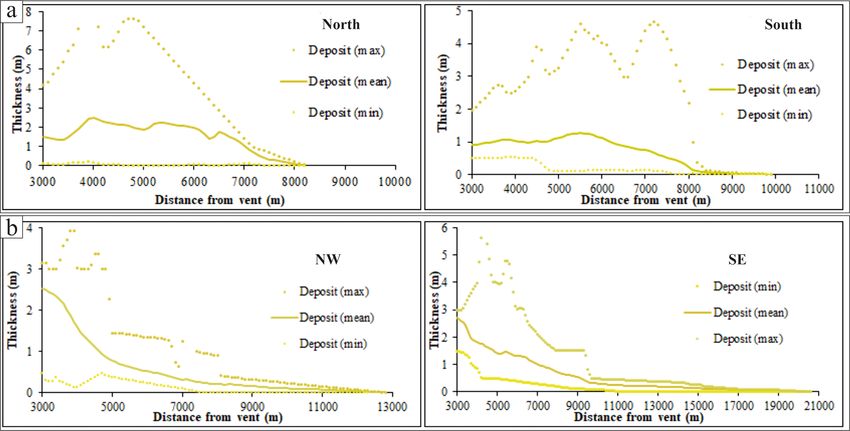
A. Tadini et al.: Reproducing pyroclastic density current deposits of the 79 CE eruption                                              125

Table 2. Calculated mean densities for each grain size for both the EU3pf and EU4b/c units.

                                                                                          8
           EU3pf
                                                  −4      −3      −2       −1         0          1      2        3      4      5
           Weighted mean density (kg m−3 )      1681     1408    1565    1650    1874         2160   2541     2550   2550   2600
                                                                                          8
           EU4b/c
                                                  −4      −3      −2       −1         0          1      2        3      4      5
           Weighted mean density (kg m−3 )      1855     1532    1804    1851    1839         2103   2519     2495   2590   2600

Figure 4. Volumetric total grain size distributions for the EU3pf and EU4b/c units.

Table 3. MSD values and related densities for the different units       we are providing minimum and maximum thicknesses along
studied.                                                                each circle in Appendix B (Fig. A1).
                                                                           Concerning the inundation area, the methodology adopted
        Unit       Sector   MSD(8)       Density (kg m−3 )              is similar to the one used by Tierz et al. (2016b) and relies on
                   All           2.34                  2327             the approach described by Fawcett (2006) and implemented
        EU3pf      N             2.19                  2305             by Cepeda et al. (2010) for landslide deposit back-analysis.
                   S             2.48                  2347             This method is based on the quantification of the areal over-
                                                                        lapping between the measured deposit (true classes) and the
                   All           2.63                  2374
        EU4b/c     NW            2.15                  2317             modelled deposit (hypothesized classes) (Fig. 5). In particu-
                   SE            3.25                  2448             lar, we quantify (a) the areal percentage of the model inter-
                                                                        secting the actual deposit (true positive – TP); (b) the areal
                                                                        percentage of the model overestimating the actual deposit
                                                                        (false positive – FP); and (c) the percentage of the model un-
3.2   Comparison between field data and simulation                      derestimating the actual deposit (true negative – TN). More
      outputs                                                           precisely,

Since the PyBox code assumes axisymmetric conditions, the                           AreaSim ∩ AreaDep
                                                                            TP =                            × 100,
thickness outputs are equal along all the radial directions of                      AreaSim ∪ AreaDep

the collapse and only vary as a function of the distance to the                     AreaSim r AreaDep
source. These output data were compared with the mean ra-                   FP =                            × 100,
                                                                                    AreaSim ∪ AreaDep
dial profiles of unit thickness (for both EU3pf and EU4b/c)
                                                                                    AreaDep r AreaSim

as derived from the digital models of deposit in Cioni et al.              TN =                             × 100.
                                                                                    AreaSim ∪ AreaDep
(2020). For building the radial profiles, the average thickness
was estimated over concentric circles drawn with a 100 m                In statistical literature, the true positive value is also called
step of distance. The radial thickness profiles were drawn              the Jaccard index of similarity (Tierz et al., 2016b; Patra et
starting from a distance of 3 km from the vent, as no thick-            al., 2020). While the TP, TN and FP approach, and in general
ness data are available for sites closer than 3 km. We ex-              the Jaccard index, focus on areal overlapping, other metrics
cluded from our analyses the portions of the circles located            can specifically focus on the distance between the boundaries
in marine areas due to the lack of reliable data. In order to de-       of the inundated areas, i.e. the Hausdorff distance, detecting
scribe the variation range of the thicknesses of the deposits,          and comparing channelized features in the deposit (Aravena

https://doi.org/10.5194/se-12-119-2021                                                                      Solid Earth, 12, 119–139, 2021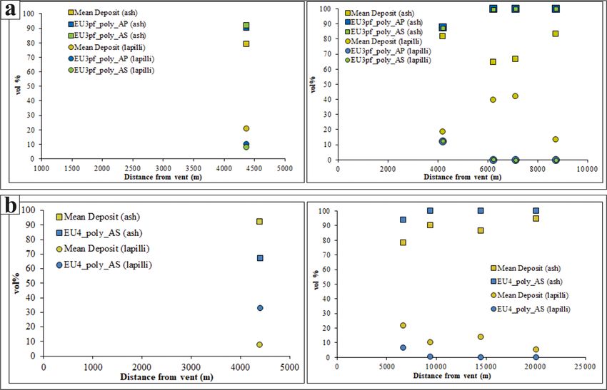
126                                 A. Tadini et al.: Reproducing pyroclastic density current deposits of the 79 CE eruption

                                                                      and between 0.1 % and 5 % (for EU4b/c). The values in Ta-
                                                                      ble 4 represent the optimal combinations.
                                                                         We adopted a simplified version of the paleo-topography
                                                                      prior to the 79 CE eruption starting from the 10 m resolution
                                                                      digital elevation model of Tarquini et al. (2007) and from the
                                                                      reconstruction given in Cioni et al. (1999) and Santacroce
                                                                      et al. (2003) (Fig. 8). The modern Gran Cono edifice and
                                                                      part of the caldera morphology have been replaced with a flat
                                                                      area, and a simplified reconstruction of the southern part of
                                                                      the Mount Somma scarp has been inserted. However, simula-
                                                                      tions performed using the unmodified digital elevation model
                                                                      (DEM) did not produce major differences.
                                                                         In the EU3pf case study, we performed both axisymmet-
                                                                      ric simulations over a round angle (given the quasi-circular
Figure 5. Sketch representing the three areas used for the valida-    shape of the deposit) and also axisymmetric–sectorialized
tion procedure (the model output outline is drawn as a dashed black   simulations to investigate possible sheltering effects of the
line).
                                                                      Mount Somma scarp (Fig. 2a). We modelled two distinct col-
                                                                      umn collapses, one to the north and the other to the south,
                                                                      each of which has a collapsed volume corresponding to the
et al., 2020). However, PyBox is not specifically aimed at            actual deposit volume in that sector. In the EU4b/c case
the replication of such features, and we focus on the areal           study, we performed only axisymmetric–sectorialized sim-
overlapping properties.                                               ulations, to reproduce more closely the dynamics of the re-
   Finally, the comparison of volume fractions of different           lated collapse, as indicated by the different dispersal in the
grain sizes has been performed using the mean value of, re-           NW and SE sectors of the PDC deposit (in particular, two
spectively, ash (< 2 mm of diameter) or lapilli (> 2 mm of di-        distinct collapses for the same simulation, one to the NW
ameter) for all the stratigraphic sections in Cioni et al. (2020)     and the other to the south-east).
placed at similar distances from the vent area. Such values              In summary we provide (a) the thickness comparison be-
were compared with the corresponding volume fractions of              tween deposit and modelled results (Fig. 6) and between sim-
the model at the same distances. In detail, we considered (i)         ulations done with a different initial volumetric fraction of
18 samples (in sectors N and S) for the EU3pf unit placed at          solid particles (ε0 – Fig. 7); (b) the inundation areas, includ-
distances from the vent area of 4 (5 N and 2 S), 6 (2 S), 7 (7        ing the quantitative matching of simulations and actual de-
S) and 9 km (2 S) and (ii) 19 samples (in sectors NW and SE)          posit (Fig. 8 and Table 5); and (c) the grain size distribution
for the EU4 unit placed at distances from the vent area of 4          comparison, between deposit and modelled values, i.e. the
(5 NW), 6 (4 SE), 9 (5 SE), 14 (4 SE) and 20 km (1 SE).               volume fractions of ash vs. lapilli (Fig. 9) and of all the grain
   The scarcity of stratigraphic sections in the N sector (for        size classes (Fig. 10).
the EU3pf unit) and the NW sector (for the EU4b/c unit) neg-
atively affects the availability of comparisons with respect to
volume fractions, which are limited to sections at 4 km of            5     Analysis and discussion
distance from the hypothetical vent area, most of which have
been collected at the bottom of paleo-valleys. Moreover, for          5.1    General considerations
the EU3pf unit, even in the S sector the available samples are
mostly concentrated in the area of Herculaneum (five sam-             Testing PyBox with respect to field data is aimed at two main
ples).                                                                objectives: (i) quantifying the degree of reproduction of the
                                                                      real PDC deposit of Plinian eruptions in terms of thickness,
                                                                      inundation area and grain size and (ii) evaluating the relia-
                                                                      bility of the code when considering different assumptions,
4   Results                                                           i.e. polydisperse vs. monodisperse situations, and 360◦ ax-
                                                                      isymmetric conditions vs. dividing circular sectors. Before
The results of six simulations (four for the EU3pf unit and           commenting on our results, two main general considerations,
two for the EU4b/c unit) are discussed here (see Table 4 for          common to both EU3pf and EU4b/c, deserve a special dis-
the main input parameters). These simulations are the result          cussion.
of an extensive investigation in which a wide range of differ-
ent values of ε0 have been tested, following a trial-and-error
procedure aimed at reproducing more closely the thickness
profile of the deposit. In particular, we performed several
simulations varying ε0 between 0.5 % and 6 % (for EU3pf)

Solid Earth, 12, 119–139, 2021                                                             https://doi.org/10.5194/se-12-119-2021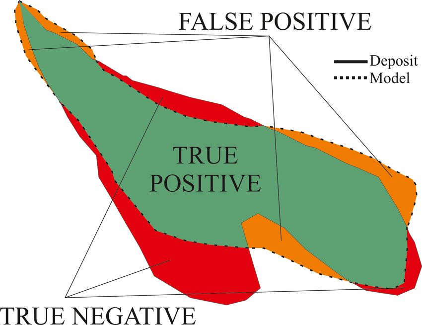
A. Tadini et al.: Reproducing pyroclastic density current deposits of the 79 CE eruption                                        127

Table 4. PyBox simulations for the EU3pf and EU4b/c units. Symbol key: AX – “axisymmetric”; AS – “axisymmetric–sectorialized”; ε0 –
“volumetric fraction of solid particles”.

                                                                              Parameters
         Unit       Simulation code
                                        Code type        Collapse type          ε0                    Grain size(s)
                    EU3pf_poly_AX       Polydisperse     Axisymmetric           5%                    TGSD
                    EU3pf_mono_AX       Monodisperse     Axisymmetric           5%                    MSD
         EU3pf
                    EU3pf_poly_ AS      Polydisperse     AX – Sectorialized     N-6 % S-3 %           TGSD-N TGSD-S
                    EU3pf_mono_AS       Monodisperse     AX – Sectorialized     N-6 % S-3 %           MSD-N MSD-S
                    EU4_poly_AS         Polydisperse     AX – Sectorialized     NW-2.5 % SE-2.5 %     TGSD-NW TGSD-SE
         EU4b/c
                    EU4_mono_AS         Monodisperse     AX – Sectorialized     NW-2.5 % SE-2.5 %     MSD-NW MSD-SE

5.1.1   Run-out truncation and non-deposited material               coarse particles), a volumetric concentration of particles of
                                                                    around 1 % (slightly lower than those used in this paper),
PyBox produces the map of the inundated area (Neri et al.,          and where ≈ 50 % or more of the particles are relatively
2015; Bevilacqua, 2016), by truncating the run-out wher-            coarse, is generally capable of producing a dense underflow
ever the kinetic energy of the flow is lower than the poten-        and a dilute, faster overriding flow. For such cases, Valentine
tial energy associated with a topographic obstacle (Sect. 2.1       (2020) suggests that a depth-averaged granular flow model
and Appendix A). In this way, however, the material that            approximates such dense underflows well and could be rea-
lies beyond the truncation is neither redistributed nor con-        sonably used for hazard assessment purposes. For the units
sidered any more. However, depending on the topography              studied here, the sedimentological features show that there
in our case study, this amount of material is not extremely         is clear evidence of the formation of a dense underflow in,
high. For instance, EU4_poly_AS (Table 4), in its SE part,          respectively, the north part of the Somma–Vesuvius volcano
has several truncations due to the intersection of the decay        (EU3pf unit; Gurioli et al., 1999), corresponding to the urban
function of kinetic energy with several topographic barriers,       settlements of Herculaneum and Pompeii (EU4 unit; Cioni et
i.e. the Apennines to the ENE and the Sorrentina Peninsula          al., 1999; Gurioli et al., 2002). However, we think the em-
to the south-east (Figs. 2 and 7). For the whole SE part of the     ployment of a box model is justified for at least the unit
deposit, the topographic barriers are located between 11.85         EU4b/c, which can be regarded as intermediate between a
and 19.25 km from vent area, with a mean value of 15 km.            dilute, turbulent and a granular concentrated current, in the
If we truncate PyBox deposit corresponding to these three           sense of Branney and Kokelaar (2002), but closer to the di-
limits, the non-deposited volume is between 3.46 × 10⁶ m3           lute endmember type. In this view, the box model can be ef-
(cut at 19.25 km) and 2.3 × 10⁷ m3 (cut at 11.85 km), with          fectively employed to describe the overriding dilute part units
a mean value of 1.27 × 10⁷ m3 (cut at 15 km). Considering           similar to the EU4, following a two-layer approach (Kelfoun,
that the volume collapsed to the south-east is 1.5 × 10⁸ m3 ,       2017; Valentine, 2020).
the non-deposited volume therefore corresponds to a value              For the box model used here, it should be kept in mind that
between 2 % and 15 %, with a mean of 8 %. The amount of             the variation in the ε0 value might have an important effect on
volume effectively “lost” is relatively small, also considering     the simulated deposit thicknesses, as seen in Fig. 7. In both
that the total volume of the collapsing mixture is inclusive of     units, in fact, the model results for thickness at the beginning
the EU4c unit (co-ignimbritic part). However, further devel-        of the simulated area (i.e. 3 km from vent area) vary from
opment of the code might consider a strategy to redistribute        ca. 1 to ca. 2 m (for EU3pf) or from ca. 1.2 to ca. 3.6 m (for
this non-deposited material (e.g. Aravena et al., 2020).            EU4b/c) if ε0 is varied, respectively, from 1.5 % to 6 % and
                                                                    from 0.5 % to 5 %.
5.1.2   Initial volumetric fraction of solid particles

The value of the initial volumetric fraction of solid parti-        5.2   Thickness comparison
cles (ε0 ) in the PDC represents one of the most uncertain
parameters, for which few constraints exist. Recently, Valen-
tine (2020) performed several multiphase simulations using          The first parameter that we compare between the deposit and
mono- or bi-disperse distributions to investigate the initia-       the modelled results is the thickness variation with the dis-
tion of PDCs from collapsing mixtures and to derive crite-          tance to the source, an approach already adopted, for in-
ria to determine when either a depth-averaged model or a            stance, by Dade and Huppert (1996). Our comparison fo-
box model are best suited to be employed for hazard mod-            cuses on the average thickness calculated over concentric
elling purposes. The author concluded that, among other             circles drawn with a 100 m step of distance. However, the
factors (e.g. impact speed or relative proportion of fine to        thickness variation in the deposit in different radial directions

https://doi.org/10.5194/se-12-119-2021                                                              Solid Earth, 12, 119–139, 2021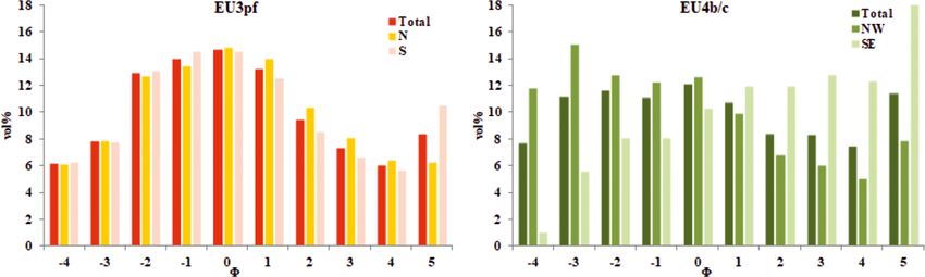
128                                A. Tadini et al.: Reproducing pyroclastic density current deposits of the 79 CE eruption

describes two different situations for the EU3pf and EU4b/c        Table 5. True positive (TP), false positive (FP) and true negative
units and deserves a brief discussion, detailed in Appendix B.     (TN) instances of the simulations in Fig. 8.
   The average thickness of the EU3pf deposit mean profile
initially shows an increasing trend (between 3 to 4 km to the            Simulation         MRL          TP      FP       TN
north and between 3 to 6 km to the south – Fig. 6a) followed                                percentile
by a slow, constant decrease. This situation could highlight                                5th          66 %    32 %     2%
a lower capability of the current to deposit in more proximal            EU3pf_mono_AX      50th         67 %    29 %     4%
areas, allowing the mass to be redistributed toward more dis-                               95th         65 %    25 %     10 %
tal sections. This could also be motivated by a spatial vari-
                                                                                            5th          63 %    37 %     0%
ation in the PDC flux regime, which was more turbulent in                EU3pf_mono_AS      50th         67 %    32 %     0.001 %
proximal areas than in distal ones, as also testified by the                                95th         75 %    24 %     0.3 %
abundance of lithofacies typical of dilute and turbulent PDCs
(//LT to xsLT; see Fig. 2b and Gurioli et al., 1999). Instead,                              5th          61 %    38 %     0.7 %
                                                                         EU4_poly_AS        50th         64 %    35 %     1%
the spatial homogeneity of lithofacies for the EU4b/c unit
                                                                                            95th         73 %    24 %     2%
(Cioni et al., 1992) suggests a higher uniformity of its par-
ent PDC. Moreover, the trend of the mean deposit thickness                                  5th          80 %    8%       11 %
profile has a steep and rapid decrease in thickness of up to             EU4_ mono_ AS      50th         78 %    7%       15 %
5–6 km, followed (after a break in slope) by a “tail” with an                               95th         73 %    3%       24 %
increasing gentler decrease in thickness. This peculiar trend
is in agreement with the lithofacies association in the unit
EU4b/c (Cioni et al., 1992), which indicates a progressive         tail part of the deposit is particularly very well reproduced
dilution of the current through time and a progressive aggra-      by the polydisperse simulations, where the simulated pro-
dation of the deposit. This trend might moreover be put in         file is almost coincident with the deposit profile (Fig. 6b –
relation to the non-exponential decay of sedimentation with        right). Conversely, to the north-west the modelled thickness
distance, described by Andrews and Manga (2012) for di-            in the initial part overestimates the real deposit a bit (Fig. 6b).
lute PDCs associated with the formation of co-ignimbritic          The polydisperse simulations (blue dashed lines in Fig. 6b)
plumes.                                                            are much closer to the measured trend of the mean thickness
   That said, the degree of matching between the modelled          profile than under the monodisperse conditions (i.e. MSD),
and the real thickness of the EU3pf unit is less accurate than     demonstrating the key role of the grain size distribution in
in the EU4b/c case study. However, the mean thickness pro-         gas-particle turbulent transport.
file of the actual deposit is roughly parallel with the model,
in some parts. Under polydisperse conditions, PyBox does           5.3     Comparison of inundated areas
not improve its performance in replicating the thickness pro-
file of EU3pf. The difficulties of PyBox in reproducing the        The areal overlapping between the model output area and the
thickness average profile reflects the likely dominant role of     actual deposit (true positive – TP) is discussed together with
the density stratification and granular transport in the deposi-   the quantification of model overestimation (false positive –
tion process in areas of complex topography (Gurioli, 1999;        FP) and underestimation (true negative – TN). In Table 5 we
Cioni et al., 2020). To the north there was in fact an extremely   also provided the TP, FP and TN estimates for the 5th and
rough topography, similar to the present one, where the in-        95th percentiles of the maximum run-out lines (MRLs), i.e.
teraction of the PDC with the surface produced largely vari-       a measure of the spatial uncertainty affecting the actual de-
able lithofacies. To the south, by contrast, there was a gentler   posit. We remark that the TN instances could be interesting
topography, with a topographic high on which the town of           from a hazard point of view because they actually represent
Pompeii (see Fig. 2a) was built. This latter aspect is also ev-    the underestimation of the model: a conservative approach
ident from Vogel and Märker (2010), who reconstructed the          is therefore to use the lowest value of the TN instances as a
pre-79 CE paleo-topography of the plain to the south-east of       threshold to evaluate the reliability of a model.
the SV edifice. From this work, it is possible to appreciate          As said above, the polydisperse simulations of the EU3pf
how the modelled depth of the pre-79 CE surface is 0–1 m           unit poorly fit with the deposit thickness, and the inun-
lower with respect to the present surface corresponding to         dated area is significantly larger than the deposit area. Thus,
the present town of Pompeii and the ancient Pompeii excava-        they are not included in the quantitative estimation of area
tions (due to the presence of piles of tephra fallout deposits     match or mismatch. For instance, while the maximum run-
up to 2 m thick), while it is up to 6–7 m deeper to the north-     outs of the deposit are on the order of 8–10 km, the max-
west of these sites.                                               imum run-out given by the model (in the absence of to-
   The thickness comparison of the EU4b/c unit, by contrast,       pography) is ca. 13–15 km. The monodisperse simulations
suggests that this unit was likely deposited under inertial        perform better, in this sense, and maximum run-outs are
flow conditions, dominated by turbulent transport. The SE          slightly different (ca. 7–10 km) from the real ones: for this

Solid Earth, 12, 119–139, 2021                                                           https://doi.org/10.5194/se-12-119-2021
A. Tadini et al.: Reproducing pyroclastic density current deposits of the 79 CE eruption 129
Figure 6. Mean thickness comparison between the simulations (dashed lines) and the actual deposit (solid line) of (a) EU3pf and (b) EU4b/c
units. Different boxes concern different circular sectors.
reason, only the monodisperse simulations for the EU3pf posit is at an acceptable value and the percentage of model
case have been considered in Fig. 8 and Table 5. More pre- underestimation is below 2 %, the model tends to appreciably
cisely, the axisymmetric EU3pf_mono_AX and the sectorial- overestimate the median outline of the deposit. By contrast,
ized EU3pf_mono_AS share a similar degree of TP instances the simulation EU4_mono_AS shows the highest TP values
(between 63 % and 75 % – Table 5) but have opposite prop- (73 %–80 %) and the lowest FP (3 %–8 %). Despite these bet-
erties for what concerns overestimation or underestimation. ter performances, it should be kept in mind how the thickness
EU3pf_mono_AX has in fact a higher tendency to underesti- profile is less accurate under monodisperse conditions.
mate deposits (FP < TN – Table 5), while EU3pf_mono_AS Beyond 14 km (ca. 2–3 km beyond the deposit MRL95 ) the
tends to overestimate the actual deposit (FP > TN – Table 5). thickness provided by the model under polydisperse condi-
For what concerns the EU4b/c simulations (Fig. 8), we re- tions is < 1 mm (see Fig. 8c). Thin deposits might possibly
port the quantitative matching of both the simulations under be affected by erosion, and the actual deposit in the NW sec-
polydisperse and monodisperse conditions. The most strik- tor might in fact resemble the PyBox results. We also note
ing feature that could be seen from Fig. 8 is that, while to the that the MRLs defined by Cioni et al. (2020) have been de-
south-east a good match is obtained, to the north-west the fined up to the 95th percentile, meaning that there is still a
polydisperse simulation overestimates the inundation area. 5 % chance that the actual MRL could be placed further away
Conversely, the monodisperse simulation is more balanced from the source. This is very significant in the NW part of the
between NW and SE. This could be related, for the SE part, EU4b/c deposit, where no or very few outcrops can be found
to the surrounding morphology of the Sorrentina Peninsula beyond 5–6 km from vent area.
and the Apennines, which act as a natural barrier and, for the
NW sector, to the absence of morphological constraints espe- 5.4 Grain size comparison
cially to the north. The results presented in Fig. 8 and Table 5
show that the TP values for the simulation EU4_poly_AS
are in the interval 61 %–73 %, while TN values range from Finally, we consider the volume fraction of the grain sizes
0.7 % and 2 % and FP values range from 24 % and 38 %. of the actual deposits versus those derived from PyBox. We
Thus, while the degree of overlap between model and de- present the results in two different ways. Firstly, we provide
a general overview of what the relative proportions of ash or
https://doi.org/10.5194/se-12-119-2021 Solid Earth, 12, 119–139, 2021130 A. Tadini et al.: Reproducing pyroclastic density current deposits of the 79 CE eruption
Figure 8. Inundation area of the simulations of the EU3pf (a,
Figure 7. Comparison between simulations (dashed lines) assuming
b) and EU4b/c (c, d) units. The dashed lines represent the theo-
different initial volumetric fractions of solid particles (ε0 ) and the
retical isopachs (in m) of the simulated deposit. Vent location (red
actual deposit (solid line) of the (a) EU3pf unit S and (b) EU4b/c
triangle), vent uncertainty area (red line) and SV caldera (orange
unit SE. In (b), the inset is a magnification of the thicknesses more
dashed line) as in Tadini et al. (2017). MRLs as in Fig. 3. The DEM
than 9 km from the vent.
used in the simulations and as a background derives from Tarquini
et al. (2007) according to the modifications explained in Sect. 4.
lapilli are with distance to the source (Fig. 9), and then we
shift of ca. 2 8 toward the finer grain sizes in the modelled
provide more complete volumetric grain size comparisons
data.
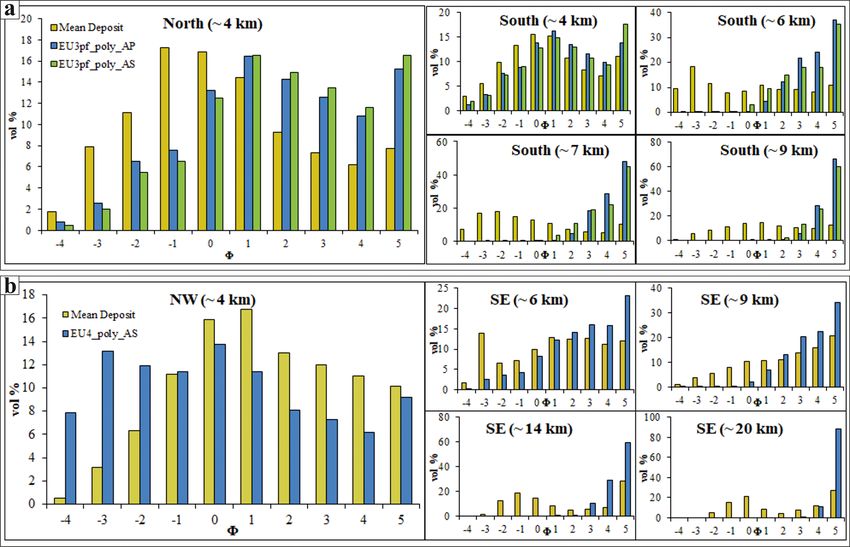
for each 8 unit (Fig. 10). This comparison is one of the most
For the EU4b/c unit, we observe that the general propor-
uncertain because of some inherent epistemic uncertainties in
tions between ash and lapilli (Fig. 9b) are more similar be-
the data: (i) the complete lack of ultra-proximal sites possibly
tween the model and the deposit (especially at 4 km from
enriched in coarse-grained particles that influenced the cal-
the vent area to the north). However, in Fig. 10b we see that
culated TGSD; (ii) the fact that the sections used for TGSD
at 4 km to the north, the situation is the opposite of EU3pf,
calculation and data comparison are (for both units) located
since the modelled grain size is richer in coarse particles than
mainly along the aprons of the volcano, in many cases corre-
the actual deposit. Such difference might be motivated by the
sponding to the lower parts of valleys or paleo-valleys. This
above-mentioned roughness of the topography, which might
could have led to have an underrepresentation of the finer-
favour the deposition of coarser particles at locations < 4 km.
grained deposits located in high or paleo-high morphological
In the SE sector the differences between modelled and ob-
locations.
served grain sizes are lower at 6 and 9 km distance to the
The data presented in Fig. 9 confirm the differences be-
source, while they are greater at 14 and 20 km, where the
tween EU3pf and EU4b/c. EU3pf (Fig. 9a) shows that the
two finest modelled grain sizes account for > 80 % of the
simulated and real volumetric contents of ash or lapilli are
volume.
similar only up to 4 km (both to the north and to the south).
Then, the relative proportions of ash or lapilli in the simula-
tions indicate that, after 6 km, the simulated grain sizes are 6 Conclusions
made almost entirely (> 90 %) by ash, with a sensitive dif-
ference with respect to field data (only to the south, as to We have evaluated the suitability of the box-model approach
the north there are no available measurements). The most ex- implemented in the PyBox code to reproduce the deposits of
treme situation could be seen at 9 km, where the modelled EU3pf and EU4b/c, two well-studied PDC units from dif-
grain sizes are composed for > 80 % in volume by the two ferent phases of the 79 CE Pompeii eruption of Somma–
finest ones (4–5 8), while deposit data indicate a more equal Vesuvius (Italy). The total volume, the TGSD, the grain
distribution of grain sizes. In Fig. 10a we observe that at 4 km densities and the temperature obtained from the field data
(both N and S) the grain size distributions are similar be- are used as the main inputs of PyBox. The model produces
tween the actual deposit and the model, although there is a several outputs that can be directly compared with the in-
Solid Earth, 12, 119–139, 2021 https://doi.org/10.5194/se-12-119-2021A. Tadini et al.: Reproducing pyroclastic density current deposits of the 79 CE eruption 131
Figure 9. Volumetric content of ash or lapilli of model or deposit with distance to the source of the units (a) EU3pf N/S (left and right,
respectively) and (b) EU4b/c NW/SE (left and right, respectively).
undation areas and radially averaged PDC deposit features, of TP instances (between 63 % and 75 %) but have oppo-
namely the unit thickness profile and the grain size distribu- site properties for what concerns overestimation or underes-
tion as a function of the radial distance to the source. We have timation. The round-angle axisymmetric simulation underes-
performed simulations either under polydisperse or monodis- timates the actual deposit (FP < TN), while the sectorialized
perse conditions, given by, respectively, the total grain size simulation overestimates the actual deposit (FP > TN). (3)
distribution and the mean Sauter diameter of the deposit. We The simulated and real volumetric contents of ash or lapilli
have tested axisymmetric collapses either as round angle or in EU3pf are similar only up to 4 km. Then, the relative pro-
divided into two circular sectors. The initial volumetric frac- portions of ash or lapilli in the simulations indicate that the
tion ε0 of the solid particles over the gas is the main tuning simulated grain sizes are made up almost entirely (> 90 %)
parameter (given its uncertainty) that is explored to fit the by ash, with a sensitive difference with respect to field data
outputs with the field data. In this study, we obtained the best after 6 km. We observe that at 4 km the grain size distribu-
fit of deposit data with a plausible initial volume concentra- tions are similar between the actual deposit and the model,
tion of solid particles from 3 % to 6 % for EU3pf (depending although there is a shift of ca. 2 8 toward the finer grain sizes
on the circular sector) and of 2.5 % for EU4b/c. These con- in the modelled data.
centrations optimize the reproduction of the thickness profile Concerning instead the EU4b/c unit, (1) this unit has a
of the actual deposits. steep and rapid decrease in thickness of up to 5–6 km, fol-
Concerning the EU3pf unit, (1) the average thickness of lowed, after a break in slope, by a tail with a gentler de-
the EU3pf deposit initially shows an increasing trend, from 3 crease in thickness. The polydisperse box-model simulations
to 4 km to the north and from 3 to 6 km to the south, fol- are much closer to the measured trend of the mean thick-
lowed by a slow, constant decrease. The simulated thick- ness profile than under the monodisperse conditions. The SE
ness poorly resembles the actual deposit, although the maxi- thickness profile of the polydisperse simulation is almost co-
mum values are comparable and the two profiles are roughly incident (within the uncertainty range) with the correspond-
parallel, in some parts. Under polydisperse conditions, Py- ing part of the deposit (specifically after 6 km and with a ca.
Box does not improve its performance in reproducing the 0.5 m overestimation between 3.5–6 km), while to the north-
thickness profile of EU3pf. (2) In the monodisperse simu- west the modelled thickness slightly overestimates the real
lations of EU3pf the maximum run-outs are slightly differ- deposit in the initial part (up to ca. 6 km). (2) In the simula-
ent from the real ones, but overall consistent. The round- tions of EU4b/c, a good match of inundated area towards the
angle and sectorialized simulations share a similar degree south-east is obtained. Towards the north-west the polydis-
https://doi.org/10.5194/se-12-119-2021 Solid Earth, 12, 119–139, 2021132 A. Tadini et al.: Reproducing pyroclastic density current deposits of the 79 CE eruption Figure 10. Comparison of volumetric grain sizes of the (a) EU3pf and (b) EU4b/c units. Different boxes concern different distances to the source. perse simulation sensibly overestimates the inundation area. icantly different sedimentological features and should likely By contrast, the simulation under monodisperse conditions be better described by different models. The study findings shows the highest TP values (73 %–80 %) and the lowest FPs indicate that the box model, which is suited to describe tur- (3 %–8 %). However, the thickness profile is less accurate un- bulent particle-laden inertial gravity currents, describes the der monodisperse conditions. Moreover, thin deposits in the EU4b/c PDC unit well but is not able to accurately catch NW sector might possibly be affected by erosion, and the ac- some of the main features of the EU3pf unit. This is probably tual deposit in the NW sector might in fact resemble the Py- due to its strongly density-stratified character, which made Box results obtained under polydisperse conditions. (3) The the interaction with the topography of the basal concentrated general proportions between ash and lapilli in EU4b/c are part of the flow a controlling factor in the deposition pro- similar in the model and the deposit. However, at 4 km to the cess. Results again highlight the key role of the grain size north, the situation is the opposite of EU3pf, since the mod- distribution in the description of inertial PDCs: while the fi- elled grain size is richer in coarse particles than the actual de- nal run-out is mostly controlled by the finest portion of the posit. In the SE sector the differences between modelled and distribution, the total grain size distribution strongly affects observed grain sizes are lower at 6 and 9 km distance to the the thickness profile (e.g. Fig. 6b), and it is an essential in- source, while they are greater at 14 and 20 km, where the two gredient for proper modelling of the PDC dynamics. finest modelled grain sizes account for > 80 % of the volume. Our study also highlights the importance of assuming ax- (4) In the SE sector, because of model run-out truncation, we isymmetric or sectorial propagation of the PDCs. This is an evaluated an average non-deposited volume of 1.27 × 10⁷ m3 additional source of uncertainty in Plinian (VEI 5) eruptions, (cut at 15 km). Considering that the volume collapsed to the in which PDCs are often generated by asymmetric column south-east is 1.5×10⁸ m3 , the average non-deposited volume collapse. In the reproduction of a specific deposit unit, con- therefore corresponds to a value of 8 %. Thus, the amount of siderations about different propagation along specific sectors volume effectively lost with the PyBox approach is relatively should be taken into account. small, also considering that the total volume of the collapsing In conclusion, while the box-model approach is certainly mixture is inclusive of the co-ignimbritic part. suited to describe large-volume (VEI > 6) low-aspect-ratio Pyroclastic density currents generated by Plinian eruptions ignimbrites, some care should be taken when it is applied span a wide range of characters and can display very different to smaller PDC-forming eruptions on stratovolcanoes, since behaviour and interaction with the topography. During the the topographic effects due to flow stratification, not consid- 79 CE eruption of Somma–Vesuvius, two PDC units, despite ered by the model, might be dominantly important. However, both being emplaced after column collapses, display signif- we believe that the approach, despite its simplifying assump- Solid Earth, 12, 119–139, 2021 https://doi.org/10.5194/se-12-119-2021
You can also read