Stress-strain characterization of seismic source fields using moment measures of mechanism complexity
←
→
Page content transcription
If your browser does not render page correctly, please read the page content below
Geophys. J. Int. (2021) 227, 591–616                                                                                  https://doi.org/10.1093/gji/ggab218
Advance Access publication 2021 June 05
GJI Seismology

Stress–strain characterization of seismic source fields using moment
measures of mechanism complexity

Thomas H. Jordan and Alan Juarez
Southern California Earthquake Center, University of Southern California, Los Angeles, CA 90089–0740, USA. E-mail: tjordan@usc.edu

Accepted 2021 June 2. Received 2021 March 12; in original form 2021 May 7

                                                                                                                                                            Downloaded from https://academic.oup.com/gji/article/227/1/591/6293847 by guest on 27 November 2021
                                       SUMMARY
                                       Earthquake ruptures and seismic sequences can be very complex, involving slip in various
                                       directions on surfaces of variable orientation. How is this geometrical complexity in seismic
                                       energy release, here called mechanism complexity, governed by tectonic stress? We address this
                                       question using a probabilistic model for the distribution of double couples that is consistent with
                                       three assumptions commonly used in regional stress inversions: the tectonic stress is constant,
                                       slip vectors are aligned with the maximum shear traction in the plane of slip, and higher
                                       shear traction promotes more seismic energy release. We characterize the moment-tensor field
                                       of a stress-aligned source process in terms of an ordered set of principal-stress directions, a
                                       stress shape factor R, and a strain-sensitivity parameter κ. The latter governs the dependence
                                       of the seismic moment density on the shear-traction magnitude and therefore parametrizes
                                       the seismic strain response to the driving stress. These stress–strain characterization (SSC)
                                       parameters can be determined from moment measures of mechanism complexity observed in
                                       large earthquakes and seismic sequences. The moment measures considered here are the ratio of
                                       the Aki moment to the total seismic moment and the five fractions of the total-moment defined
                                       by linear mappings of the moment-tensor field onto an orthonormal basis of five deviatoric
                                       mechanisms. We construct this basis to be stress-oriented by choosing its leading member to
                                       be the centroid moment tensor (CMT) mechanism and three others representing orthogonal
                                       rotations of the CMT mechanism. From the projections of the stress-aligned field onto this
                                       stress-oriented basis, we derive explicit expressions for the expected values of the moment-
                                       fraction integrals as functions of R and κ. We apply the SSC methodology to a 39-yr focal
                                       mechanism catalogue of the San Jacinto Fault (SJF) zone and to realizations from the Graves–
                                       Pitarka stochastic rupture model. The SJF data are consistent with the SSC model, and the
                                       recovered parameters, R = 0.45 ± 0.050 and κ = 5.7 ± 1.75, indicate moderate mechanism
                                       complexity. The parameters from the Graves–Pitarka realizations, R = 0.49 ± 0.005, κ =
                                        9.5 ± 0.375, imply lower mechanism complexity than the SJF catalogue, and their moment
                                       measures show inconsistencies with the SSC model that can be explained by differences in the
                                       modelling assumptions.

                                       Key words: Statistical methods; Earthquake dynamics; Earthquake hazards; Earthquake
                                       source observations; Theoretical seismology; Mechanics, theory, and modelling.

1 I N T RO D U C T I O N

How faulting relates to tectonic stress is a long-standing geophysical problem (Anderson 1905; Wallace 1951; Bott 1959; McKenzie 1969;
Isacks & Molnar 1971; Zoback et al. 1987; Matsu’ura et al. 2019). Tectonic stresses are latent variables that are not directly measurable but
must be inferred from observations of deformation at appropriate scales. One widely applied technique is to invert a regional distribution of
earthquake focal mechanisms or moment tensors for a normalized deviatoric (reduced) stress tensor (e.g. Gephart & Forsyth 1984; Michael
1984, 1987; Lund & Slunga 1999; Angelier 2002; Hardebeck & Michael 2006; Terakawa & Matsu’ura 2008; Vavryčuk 2014; Martı́nez-Garzón
et al. 2016). These inversion algorithms are based on three assumptions:


C The Author(s) 2021. Published by Oxford University Press on behalf of The Royal Astronomical Society. This is an Open Access

article distributed under the terms of the Creative Commons Attribution License (http://creativecommons.org/licenses/by/4.0/), which
permits unrestricted reuse, distribution, and reproduction in any medium, provided the original work is properly cited.                              591
592      T.H. Jordan and A. Juarez

   1. The mean tectonic stress averaged over the region represents the local stress; any fluctuations in stress are small and randomly distributed
about this mean.
   2. On average, slip vectors are oriented in the direction of the shear traction across the fault surface; angular deviations from this optimal
direction are small and average to zero.
   3. Ruptures can occur on fault surfaces with arbitrary orientations, but the likelihood of seismic energy release is greater on surfaces with
higher shear tractions.

     In this paper, we develop a statistical model for the distribution of double couples consistent with these assumptions. The model allows us
to characterize the stress state and inelastic strain response of earthquakes and seismic sequences from observations of mechanism complexity
based on seismic-moment partitioning.

1.1 Source mechanism complexity

                                                                                                                                                       Downloaded from https://academic.oup.com/gji/article/227/1/591/6293847 by guest on 27 November 2021
Mechanism complexity is the term we use to indicate variability in the orientation of fault planes and slip vectors during the seismic
source process. Our model assumes that the local release of seismic energy can be described by a double-couple (DC) moment tensor (an
elementary shear dislocation), so that the moment-tensor field representing an extended seismic source—the stress glut of Backus & Mulcahy
(1976a, b)—is a space–time superposition of DCs. The source mechanism is simple if the stress glut is everywhere proportional to the
same DC. The source variability is then completely specified by a scalar moment density, and the integral of that density over the source
volume—the Aki (ordinary) seismic moment—is equal to the total moment.
      The mechanism of an extended seismic source is complex if the fault-plane and slip-vector orientations vary with position and time.
In that case, some fraction of the seismic moment cancels out of the integrated moment tensor, and the Aki moment is less than the total
moment. The relative difference between the total seismic moment and the Aki moment is thus one measure of source complexity (Jordan &
Juarez 2019, 2020).
      The mechanism complexity of large earthquakes—often called geometrical complexity (e.g. Rivera & Kanamori 2014; Romanet et al.
2018)—can be kinematically parametrized by discretizing the stress glut into a finite set of planar fault patches of specified area, orientation and
slip history (e.g. Graves & Pitarka 2016; Mai et al. 2018). Records of large earthquakes on seismographic and geodetic arrays, in combination
with geologic information about local fault structure, have been inverted for subevent sequences with plausible rupture trajectories (e.g. Wald
& Heaton 1994; Hauksson et al. 2011; Meng et al. 2012; Mai & Thingbaijam 2014; Koketsu 2016; Somala et al. 2018). Recent exemplars
of finite-fault modelling include studies of the exceptionally complex M 7.8 Kaikōura earthquake of 14 November 2016 (Cesca et al. 2017;
Duputel & Rivera 2017; Hamling et al. 2017; Wang et al. 2018).
      An alternative representation of mechanism complexity decomposes the stress glut into orthogonal moment-tensor fields (Jordan &
Juarez 2019, 2020). The stress glut is projected onto an orthonormal set of source mechanisms that span the 6-D space of all possible moment
tensors. Each mechanism in this basis is constant over the source volume and defines a scalar moment field. Some of these fields may have
zero measure, in which case the dimension of the moment-tensor space can be reduced. For example, our assumption that the elementary
source mechanisms are DCs implies that the stress glut is purely deviatoric, so that the rank of the stress glut is at most five.
      In previous papers (Jordan & Juarez 2019, 2020), we investigated orthonormal bases in which the leading member is the source
mechanism of the centroid moment tensor (CMT)—the moment-weighted mean mechanism, defined to be the space–time integral of the
stress glut normalized by the Aki seismic moment. The projection of the stress glut onto the CMT mechanism maps the space–time evolution
of the source into a scalar field and defines the zeroth-degree moment-tensor field. This constant-mechanism approximation is often used
in the low-frequency estimation of characteristic source dimensions and directivity parameters (Bukchin 1995; McGuire et al. 2001, 2002;
Clévédé et al. 2004; Chen et al. 2005; McGuire 2017), but its efficacy in describing seismic radiation at high frequencies is limited (Aochi
& Madariaga 2003; Graves & Pitarka 2016; Mai et al. 2018).
      Mechanism complexity can be quantified by projecting the stress glut onto the basis members orthogonal to the CMT. We have shown
how a unique fraction of the total moment can be allocated to each basis member by a mapping that defines the total-moment simplex for the
basis set (Jordan & Juarez 2019, Section 5). This new type of total-moment accounting plays a central role in the theory developed in this
paper, and its formulation is reviewed in the Section 3.
      Our emphasis in Jordan & Juarez (2019, 2020) was on the process of sequentially adding basis members that could account for
the low-order polynomial moments of the residual stress glut; for example the difference between stress glut and its constant-mechanism
approximation. We set up a progressive Bayesian scheme for inverting seismic data to estimate multipoles higher than the CMT monopole,
which we have applied to the 2016 Kaikōura earthquake (Juarez & Jordan 2020).
      Here we shift our focus to the forward problem of predicting mechanism complexity under assumed stress conditions. Assumptions
(1) and (2) are used in the inversion of regional seismicity catalogues for stress-ellipsoid orientations and shape parameters. Assumption (3)
has been incorporated into some stress-inversion algorithms but, to our knowledge, only implicitly. For example, the objective function in
Michael’s (1984) inversion scheme penalizes tractions that differ from a common, normalized value, which favors larger tangential tractions.
      We explicitly incorporate assumption (3) into our model by introducing a ‘strain-sensitivity factor’ that relates the probability of slip
on a fault element to the magnitude of the shear traction acting across it. This positive parameter characterizes the seismic inelastic strain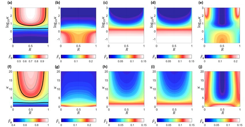
Stress-strain characterization           593

response to stress and, together with the stress shape parameter, determines the mechanism complexity. Inversion of the moment measures to
estimate these quantities is what we mean by the stress–strain characterization (SSC) of a seismic source field.

1.2 Organization
The SSC method developed in this paper can be applied to arbitrary superposition of seismic sources, including large earthquakes as well
as extended source fields comprising seismic clusters and regional seismicity. Section 2 sets up the notation of deviatoric moment-tensor
fields that represent individual earthquakes and catalogueed sequences. Section 3 describes the representation of these fields by basis sets of
orthogonal mechanisms and reviews the total-moment simplex defined by a basis set.
      Section 4 develops a probabilistic model of mechanism complexity in which the elementary stress-aligned DCs of arbitrary orientation
are exponentially distributed with the shear-traction magnitude. The strain-sensitivity factor scales the normalized traction; increasing this
sensitivity concentrates the energy release into optimal mechanisms and decreases mechanism complexity.
      In Section 5, a stress-oriented basis set is constructed by requiring the CMT mechanism to be its leading member. Under the SSC

                                                                                                                                                          Downloaded from https://academic.oup.com/gji/article/227/1/591/6293847 by guest on 27 November 2021
assumptions, this tensor defines the stress-oriented reference frame. We then select the other basis members to represent orthogonal rotations
about the CMT axes. We solve the forward problem by deriving integral expressions for the expected total-moment fractions of the stress-
oriented basis, and we set up the inverse problem by showing how these measures of mechanism complexity depend on the differential stress
ratio and the strain-sensitivity factor.
      In Section 6, we construct a likelihood function for the SSC parameters that accounts for the covariances among the observations.
We apply the SSC methodology to a 39-yr moment-tensor catalogue of the San Jacinto Fault (SJF) zone of Southern California. We obtain
maximum-likelihood estimates of the stress parameters consistent with previous studies, as well as novel estimates of mechanism complexity
and the strain sensitivity to stress implied by this complexity. We also use the moment measures to compare the SSC model with the Graves
& Pitarka (2016) stochastic rupture model, highlighting the statistical differences between the two models.

2 MOMENT-TENSOR FIELDS
A moment-tensor field is a space–time distribution of second-order, symmetric tensors used in the kinematic representation of seismic sources
(Backus & Mulcahy 1976a, b). At every space–time point (r, t) in the finite space–time source volume V = R × T, we express the moment
tensor field as a non-negative scalar-moment density times a source-mechanism density, m (r, t) = m(r, t) m̂(r, t). The scalar moment
                                                                                   √           √
density is the Frobenius (Euclidean) norm of moment-tensor field, m = m = m : m = m i j m i j , and the local source mechanism m̂
is a symmetric, second-order tensor with unit norm, m̂ : m̂ = 1.
      The space of all moment tensors M can be mapped to the 6-D Euclidean vector space R6 by a norm-preserving isomorphism, which
allows us to treat mechanisms as unit vectors in R6 (Silver & Jordan 1982). The most general source field includes an isotropic component,
for example from crack opening (Matsu’ura et al. 2019), but here we assume the field is purely deviatoric, tr [m̂] = 0, which reduces M to
the five-dimensional space of deviatoric moment tensors, denoted MD . Deviatoric mechanisms are points on the unit hypersphere in MD .
      The total moment of any moment-tensor field is defined to be the integral of the scalar moment density (Jordan & Juarez 2019),

MT :=           m(r, t) dr dt =        m (r, t) dr dt.                                                                                  (1)
         T   R                       T   R
For an elastic dislocation field, m(r, t) is proportional to the local strain energy drop, where the coefficient of proportionality is the ratio of the
average shear driving stress to the shear modulus (Kostrov 1974; Dahlen 1977; Matsu’ura et al. 2019). It has been observed that the average
apparent stress is independent of earthquake size (McGarr 1999; Ide & Beroza 2001), so MT is expected to scale with the total change in the
internal elastic energy of the source region, denoted E T .
     We consider two types of moment-tensor fields. The first is proportional to the stress-glut density (r,      ˙ t) of an earthquake rupture
(Backus & Mulcahy 1976a, b),
          1
m(r, t) = √ ˙ (r, t) .                                                                                                                            (2)
           2
The space–time integral of this density (its zeroth polynomial moment) is the net moment tensor,

M0 := μ(0) (m) =         m (r, t) dr dt,                                                                                                           (3)
                    T   R

and its size is the net seismic moment, here called the Aki moment,


M0 :=          m  (r, t) dr dt  = M0 : M0 .
                                                                                                                                                  (4)

         T   R

M0 is the norm of the integral, whereas MT is the integral of the norm. By the Cauchy–Schwarz inequality, M0 ≤ MT .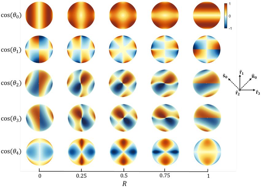
594        T.H. Jordan and A. Juarez
                        √
      We note that√the 2 factor in eq. (2) arises from Aki’s (1966) original definition of seismic moment, which pegs the scalar density of
the stress glut at 2m(r, t). In our notation, √  the moment tensor defined by the zeroth moment of the stress glut—the usual seismic moment
tensor (Aki & Richards 2002)—is therefore 2 times the net moment tensor M0 .
      The centroid (r0 , t0 ) of a moment tensor field is the space–time point that minimizes the norm of the first polynomial moment, which is
a third-order tensor (Backus 1977),

μ(1) (m) =        m (r, t) (r − r0 ) dr (t − t0 ) dt .                                                                                     (5)
               T R

The CMT is the monopole approximation of m that concentrates the energy release at the source centroid (Dziewonski et al. 1981):
m(r, t) ≈ M0 δ(r − r0 )δ(t − t0 ), where δ(·) is the Dirac delta function. We refer to the normalized moment tensor, M̂0 = M0 /M0 , as the CMT
source mechanism. The CMT mechanism is the moment-weighted mean of the local source mechanisms m̂(r, t). Accurate estimations of the
CMT are now available at low magnitude thresholds both globally (Ekström et al. 2012) and regionally (e.g. Hutton et al. 2010; Godey et al.
2013; Ross et al. 2017; Aoi et al. 2020).
     The second type of moment-tensor field is a discrete distribution of seismic events within a region R and time interval T, such as the

                                                                                                                                                                 Downloaded from https://academic.oup.com/gji/article/227/1/591/6293847 by guest on 27 November 2021
seismicity of a deformation zone (e.g. Terakawa & Matsu’ura 2008; Bailey et al. 2010), an aftershock sequence (e.g. Beroza & Zoback 1993;
Shearer et al. 2003; Hardebeck 2020), or a multiple CMT representation of a single earthquake (e.g. Tsai et al. 2005; Mai & Thingbaijam
2014). We assume the individual events are small enough and simple enough to be represented by deviatoric CMTs, so that the field comprises
N point sources with moment tensors mn ∈ MD , seismic moments m n , and source mechanisms m̂n :

              N
                                                     N
m(r, t) =           mn δ (r − rn ) δ (t − tn ) =           m n m̂n δ (r − rn ) δ (t − tn ) .                                                              (6)
              n=1                                    n=1

In this case, the discretized field is represented by a CMT catalogue C = {rn , tn , m n , m̂n : n = 1, . . . , N }, and the moment tensor of eq.
(3) reduces to a Kostrov summation,

        N
M0 =          mn .                                                                                                                                        (7)
        n=1


                                                             N
The Aki moment of this discrete field, M0 =                      (M̂0 : m̂n )m n , thus scales with the net inelastic strain (Kostrov 1974), whereas its total
                                                             n=1

                      N
moment, MT =               m n , scales with the total energy release E T .
                     n=1

3 MOMENT MEASURES OF MECHANISM COMPLEXITY

Any deviatoric moment-tensor field m(r, t) ∈ MD can be represented as a linear combination of up to five mutually orthogonal source
mechanisms. The minimum number of mechanisms required to support the moment-tensor density equals the rank of the field, denoted D. It
will be convenient to define the reduced dimension d = D − 1; for example a deviatoric source mechanism m̂ is a vector on the d-sphere,
which is the unit hypersphere in MD (Silver & Jordan 1982). In this section, we allow the dimensionality to be variable, but in our theoretical
development of the SSC model, we will focus on the general deviatoric case, where D = 5 and d = 4.
     We choose the CMT mechanism M̂0 to be the leading (zeroth-degree) basis member, and we complete the basis by defining d orthogonal
mechanisms {M̂α } indexed by a degree number α = 1, . . . , d. The complete basis set, representing the D degrees of moment-tensor
freedom, are normalized to unit length,

M̂α : M̂β = δαβ , α, β = 0, . . . , d.                                                                                                                    (8)

Hence, the basis projections of the local source mechanism m̂ define the direction-cosine fields,

cos θα (r, t) := M̂α : m̂ (r, t) ,                                                                                                                        (9)

which give the coordinates of m̂ on the d-sphere. The moment-tensor density can be written as the sum over the basis members,

                           d
m(r, t) = m (r, t)             M̂α cos θα (r, t) .                                                                                                       (10)
                        α =0

The particular (stress-oriented) basis set used in this paper for the SSC of moment-tensor fields is described in Section 5.
     The squares of the direction cosines form a d-simplex; that is they are D = d + 1 positive numbers that sum to unity at each space–time
point,

d
       cos2 θα (r, t) = 1.                                                                                                                               (11)
α =0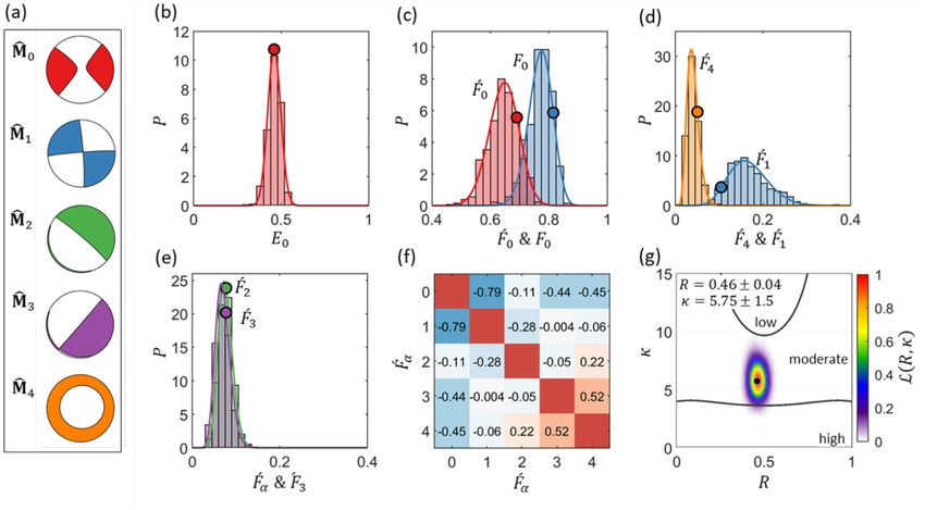
Stress-strain characterization         595

The substitution of (11) into (1) decomposes the total moment into D fractional moments,

        d

MT =          Mα.                                                                                                                             (12)
        α=0

The fractional moment of degree α is the integral of the scalar moment density weighted by the square of the direction cosine,


M α :=        m (r, t) cos2 θα (r, t) dr dt, α = 0, . . . , d.                                                                                (13)
        T     R

      The partitioning of the scalar density m(r, t) into moment fractions by eq. (13) depends on the local source orientation m̂ but not m itself.
This choice is consistent with our interpretation that MT scales with the total elastic energy change E T ; that is, all elementary sources add to
E T in proportion to their scalar seismic moments, regardless of their orientation. An alternative is quadratic (2-norm) moment partitioning,
in which the integral of |M̂α : m(r, t)|2 defines the square of the degree-specific moment. Combining moments quadratically is inconsistent
with the additive energy interpretation, however. Therefore, we adopt the simplex (1-norm) measure given by eq. (13).
      Normalizing the expressions (12) and (13) by MT defines the total-moment simplex (Jordan & Juarez 2019),

                                                                                                                                                      Downloaded from https://academic.oup.com/gji/article/227/1/591/6293847 by guest on 27 November 2021

        Mα
             d

Fα :=     ,      Fα = 1.                                                                                                                      (14)
        MT α = 0

Fα is the total-moment fraction of degree α, which we associate with the fraction of the seismic energy released with mechanism M̂α . If the

mechanism m̂ is constant throughout the source volume, F0 = 1 and Fα = 0 for α ≥ 1. A value of F0 close to unity thus indicates a simple
mechanism. By the same token, its complement,
       d
                          1
F+ :=      Fα = 1 − F0 =                m (r, t) sin2 θ0 (r, t) dr dt,                                                              (15)
      α =1
                             MT T R

measures mechanism complexity. In Section 5.4, we will use the 1-simplex ( F0 , F+ ) to set up a mechanism complexity scale.

     Another gauge of mechanism simplicity is the ratio of the Aki moment to the total moment, F0 := M0 /MT . The moment measures F0
and F0 are closely related quantities, but they are not equal. The Aki moment M0 is the integral of the scalar moment density weighted by the
zeroth-degree direction cosine, rather than by the square of this cosine,

M0 =        m (r, t) cos θ0 (r, t) dr dt .                                                                                               (16)
        T R

If the mechanism complexity is small ( F+   1), then the expected value of cos θ0 will be close to unity, and an application of the small-angle
approximation, θ0   1, in (15) and (16) shows that

       1                  1
F0 ≈      1 + F 0 = 1 − F+ .                                                                                                               (17)
       2                   2

As the mechanism complexity increases incrementally from zero, the Aki moment fraction F0 decreases linearly with F+ , but at only half the

rate of F0 .
      Von Mises distributions with a single degree of rotational freedom have been used to investigate the expected values of the moment

fractions over the entire range of mechanism complexity, 0 < F+ < 1 (Jordan & Juarez 2019, Section 6). Here, we extend the analysis to a
statistical model of stress-aligned mechanism complexity with two degrees of rotational freedom in which the expected value is governed by
the magnitude of the resolved shear traction.

4 S T R E S S - S T R A I N C H A R A C T E R I Z AT I O N O F M O M E N T - T E N S O R F I E L D S

We develop an SSC model based on three simplifying assumptions:
   1. Shear tractions on surfaces within the source volume are specified by a constant deviatoric stress tensor . Local variations in stress are
ignored.
   2. The slip vectors of fault ruptures within the source volume are parallel to the shear traction exerted by  across the fault. Perturbations
to the stress field due to fault displacements are ignored.
   3. Slip can occur on any fault plane, but more slip is likely if the shear traction across a fault plane is higher. Dependence of the slip on
fault friction and other properties is ignored.
The SSC model is parametrized by the normalized (reduced) stress tensor ,        ˆ which orients the principal-axis reference frame and specifies
the differential stress ratio (shape factor) R, and by a strain-sensitivity factor κ, which governs the dependence of the seismic moment density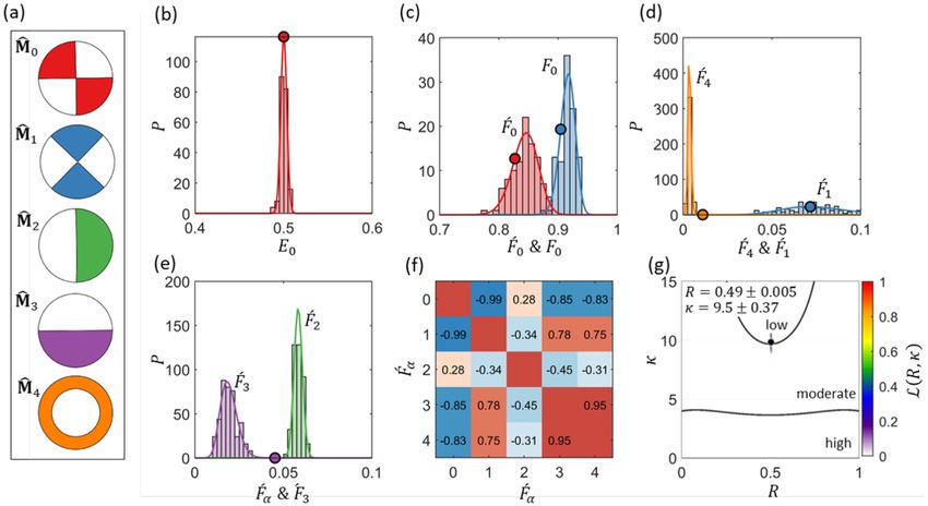
596         T.H. Jordan and A. Juarez

on the shear-traction magnitude and therefore parametrizes the inelastic strain response to stress. We show that the SSC model predicts the

Aki moment fraction F0 and the total-moment simplex { F α : α = 0, . . . , d} as functions of the stress-shape parameter R and the seismic
strain-response parameter κ.

4.1 Stress-aligned double couple

Inversion of seismicity for stress is based on the widely used concept of a stress-aligned DC (Wallace 1951; Bott 1959; McKenzie 1969;
Angelier et al. 1982; Gephart & Forsyth 1984; Michael 1984). The moment-tensor field m(r, t) of an extended seismic source is assumed
to be a space–time distribution of elementary dislocations, each described by a DC mechanism with unit fault-normal vector n̂ and unit slip
vector ŝ:
           1
m̂DC = √ [n̂ ŝ + ŝ n̂] , n̂ · ŝ = 0.                                                                                               (18)
            2
This purely deviatoric field is said to be fully aligned with the tectonic stress  if the slip vectors ŝ are everywhere parallel to the maximum

                                                                                                                                                        Downloaded from https://academic.oup.com/gji/article/227/1/591/6293847 by guest on 27 November 2021
shear tractions acting across the elementary fault planes, regardless of the fault orientation n̂. In structural geology, the alignment of fault slip
with the maximum shear traction is known as the Wallace–Bott hypothesis (Dupin et al. 1993; Célérier et al. 2012; Lisle 2013; Lejri et al.
2017), named after the first authors to apply the notion to faulting in a homogeneous medium (Wallace 1951) and to reactivated fault systems
(Bott 1959). We follow this usage by referring to a moment-tensor field in which slip is everywhere stress-aligned as a Wallace–Bott field.
     The standard derivation of a stress-aligned DC (e.g. Angelier et al. 1982) is recast here to establish our frame-invariant tensor notation.
The deviatoric stress tensor is represented in its principal-axis frame     = (r̂1 , r̂2 , r̂3 ),
 = σ1 r̂1 r̂1 + σ2 r̂2 r̂2 + σ3 r̂3 r̂3 ,                                                                                                      (19)
The principal compressive stresses sum to zero, σ1 + σ2 + σ3 = 0; they are ordered, σ1 ≥ σ2 ≥ σ3 , and interrelated by the differential stress
ratio,
       σ 1 − σ2
R :=            , 0 ≤ R ≤ 1.                                                                                                              (20)
       σ1 − σ3
The shape parameter R is used by many authors (e.g. Gephart & Forsyth 1984; Hardebeck & Michael 2006; Célérier et al. 2012), although
                                                                                                                 ˆ = Σ −1 , is normalized to
its alternative, φ = 1 − R, is also popular (e.g. Angelier et al. 1982; Lislie 2013). The reduced stress tensor,
unit length by the root-sum-square of the principal stresses,
                                   1

                      3            2

Σ :=  =                   σi2       .                                                                                                        (21)
                       i=1

      The vector normal to the fault element has principal-axis coordinates n̂ i = r̂i · n̂,where n̂ 21 + n̂ 22 + n̂ 23 = 1. The traction, τ (n̂) :=
 · n̂ = σ1 n̂ 1 r̂1 + σ2 n̂ 2 r̂2 + σ3 n̂ 3 r̂3 , can be resolved into normal and shear components,
τ(n̂) = γ (n̂) n̂ + s (n̂) .                                                                                                                    (22)
The normal traction is given by the quadratic form,
γ (n̂) := n̂ · τ (n̂) = n̂ ·  · n̂ = σ1 n̂ 21 + σ2 n̂ 22 + σ3 n̂ 23 ,                                                                          (23)
and the shear traction by the projection of τ orthogonal to n̂,
s(n̂) = (I − n̂n̂) ·  · n̂ = τ (n̂) − γ n̂.                                                                                                    (24)
      The squared norm of the shear traction across the plane with normal vector n̂ is thus the difference of two quadratic forms (Angelier
et al. 1982),
s 2 (n̂) = s(n̂)2 = τ 2 − 2γ (τ · n̂) + γ 2 = τ 2 − γ 2
                                                                               2
        = σ12 n̂ 21 + σ22 n̂ 22 + σ32 n̂ 23 − σ1 n̂ 21 + σ2 n̂ 22 + σ3 n̂ 23
        = (σ1 − σ2 )2 n̂ 21 n̂ 22 + (σ1 − σ3 )2 n̂ 21 n̂ 23 + (σ2 − σ3 )2 n̂ 22 n̂ 23 .                                                         (25)
     The direction of the stress-aligned slip vector is ŝ (n̂) = s −1 (n̂)s(n̂). The corresponding stress-aligned DC mechanism, expressed in the
form (18), is the unit symmetric tensor,
                                                ⎡                                                       ⎤
                                                  2ŝ n̂     ŝ1 n̂ 2 + ŝ2 n̂ 1 ŝ1 n̂ 3 + ŝ3 n̂ 1
              1                             1 ⎢ 1 1                                                     ⎥
m̂ (n̂) : = √ [n̂ ŝ (n̂) + ŝ (n̂) n̂] = √ ⎣ ·                    2ŝ2 n̂ 2       ŝ2 n̂ 3 + ŝ3 n̂ 2 ⎦                                    (26)
               2                             2       ·                 ·                  2ŝ3 n̂ 3
                   ⎡                                                                                      ⎤
                     2 (σ1 − γ ) n̂ 1 n̂ 1 (σ1 + σ2 − 2γ ) n̂ 1 n̂ 2 (σ1 + σ3 − 2γ ) n̂ 1 n̂ 3
               1 ⎢                                                                                        ⎥
           = √ ⎣              ·               2 (σ2 − γ ) n̂ 2 n̂ 2           (σ2 + σ3 − 2γ ) n̂ 2 n̂ 3 ⎦ .
               2s             ·                        ·                        2 (σ3 − γ ) n̂ 3 n̂ 3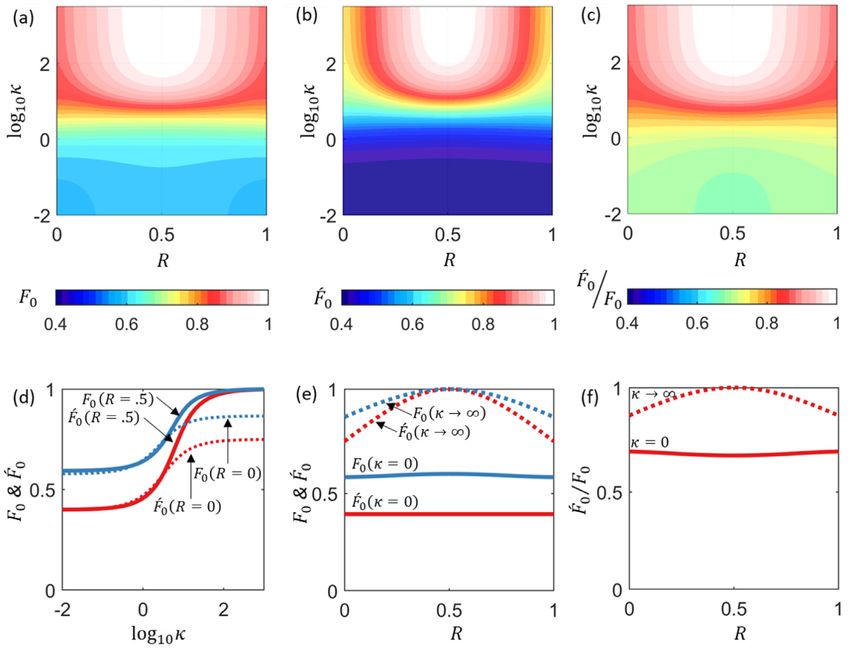
Stress-strain characterization   597

Figure 1. Shear traction s(n̂) plotted on the upper hemisphere of S1 for selected values of R. The projection is orthogonal to r̂2 .

The Wallace–Bott mechanism given by (26) is the DC that maximizes the shear traction s on a fault with normal n̂. Some algebra shows that
the inner product of this mechanism with the reduced stress tensor is proportional to the shear traction resolved on the fault plane,
                                            √
               √      3
                          σi σi − γ             2
ˆ : m̂ (n̂) = 2                     n̂ i2 =     s (n̂) .                                                                            (27)

                                                                                                                                                         Downloaded from https://academic.oup.com/gji/article/227/1/591/6293847 by guest on 27 November 2021
                     i =1
                          Σ      s            Σ

     The shear traction s(n̂) is plotted on the unit sphere S1 for selected values of R in Fig. 1. Here we have scaled the stresses such that the
average shear stress in the 1–3 plane, which equals the maximum of the shear traction on any plane, is unity for all 0 < R < 1,
                          σ1 − σ3
s0 = max s (n̂) =                 = 1.                                                                                                            (28)
       n̂ ∈ S1               2
With this normalization, the principal stresses are completely determined by R,
        2                             2                               2
σ1 =       (1 + R) , σ2 = − (2R − 1) , σ3 = − (2 − R) ,                                                                                           (29)
        3                             3                               3
and the shear-traction magnitude and the squared stress modulus become,

s (n̂; R) = 2 R 2 n̂ 21 n̂ 22 + n̂ 21 n̂ 23 + (1 − R)2 n̂ 22 n̂ 23 ,                                                                              (30)

             8                                     4
 2 (R) =       1 − R + R 2 = 2 1 + (R − 1/2)2 .                                                                                                  (31)
             3                                     3
       If 0 < R < 1, the non-negative scalar field s(n̂) has 18 stationary points on S1 . It vanishes if n̂ is a principal axis of ; that is at the 6
points where n̂ = ±r̂i . The stress magnitude has eight saddle points at n̂ = √12 (±r̂i ± r̂2 ), where i = 1 or 3, and it achieves its maximum
value of unity at 4 points that lie in the 1–3 plane, which we label as ±n̂0 , ±ŝ0 . The two orthogonal directions,
       1                      1
n̂0 = √ (r̂1 + r̂3 ) , ŝ0 = √ (r̂1 − r̂3 )                                                                                     (32)
        2                      2
are the normal and slip vectors of the optimal DC of , defined to be the Wallace–Bott mechanism where the shear traction reaches its
maximum value of s0 = 1:
       1
  0 = √
M̂DC      (n̂0 ŝ0 + ŝ0 n̂0 ) .                                                                                                                  (33)
        2
The null axis of the optimal DC is b̂0 = −n̂0 × ŝ0 = r̂2 .
     The end-member cases R = 0 ( σ1 = σ2 ) and R = 1 ( σ2 = σ3 ) are degenerate. At these limits, the locus where s achieves its
maximum value s0 = 1 dimensionally inflates from four discrete points to two small circles at latitudes of ±π/4 from the stress symmetry
plane; s vanishes at the pole and equator of this plane (Fig. 1). This degeneracy leads to a singular behavior at R = 0, 1 for some of the
moment measures (see Section 5.3), but these singularities can be handled by defining the stress states at R = 0, 1 to be the limiting states
as R → 0, 1.

4.2 SSC model

If
   ˆ is constant throughout the source volume, the Wallace–Bott mechanism (26) is a function of only its fault-orientation vector; therefore,
any Wallace–Bott field is completely specified by a scalar moment density m(r, t) and a vector field of fault orientations n̂(r, t),
m(r, t) =        m (r, t) m̂ (n̂ (r, t)) ,                                                                                                       (34)
To formulate the SSC model, we represent the spatiotemporal source process and its response to the stress field in terms of probability
distributions. The scalar moment density normalized by the total moment is a non-negative function that integrates to unity over the source
space–time volume:

             1
 f (r, t) :=    m (r, t) ≥ 0,        f (r, t) dr dt = 1.                                                                               (35)
             MT
                                       T      R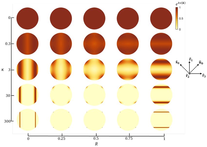
598         T.H. Jordan and A. Juarez

We can think of this distribution as a probability density function (p.d.f.) on V that defines the moment-weighted expectation of a general
source function g(r, t):

E f [g] :=       f (r, t) g (r, t) dr dt.                                                                                              (36)
             T       R

In particular, the moment-weighted expectation of the source mechanism under f is the product of its Aki moment fraction and its CMT
mechanism,

E f [m̂ ] = F0 M̂0 .                                                                                                                         (37)

Projecting (37) onto M̂0 shows that the Aki moment fraction is the expectation of the zeroth-degree direction cosine, E f [cos θ0 ] = F0 . By
definition, E f [cos θα ] = 0 for α ≥ 1. Similarly, the total-moment fractions corresponding to the basis expansion of eq. (10) are the expected
values of the squared direction cosines,

E f cos2 θα = Fα .                                                                                                                          (38)

                                                                                                                                                      Downloaded from https://academic.oup.com/gji/article/227/1/591/6293847 by guest on 27 November 2021
      The fault orientation field n̂(r, t) maps the source volume onto the fault-orientation sphere, V → S1 . The expectation of any orientation
field g(n̂) under f can thus be expressed as an integral over S1 ,

E f [g] = Es [g] :=    ps (n̂) g (n̂) dn̂.                                                                                                  (39)
                         S1

The p.d.f. on S1 is the moment-weighted density, ps (n̂) = Es [δ(n̂)], which is the expectation under f that the fault orientation n̂ points in a
particular direction n̂ :


ps n̂ = E f δ n̂ =           f (r, t) δ n̂ − n̂ (r, t) dr dt .                                                                           (40)
                               T R

This fault-orientation density integrates to unity because n̂ is somewhere on S1 :

   ps n̂ d n̂ =        f (r, t)   δ n̂ − n̂ (r, t) dn̂ dr dt = 1.                                                                         (41)
S1                       T R         S1

If m is a Wallace–Bott field, then the mapping of the moment density f from V to S1 via eq. (40) is well-defined and produces a unique
density ps .
     Our SSC model assumes that faults are more likely to slip if the shear traction is high. In particular, we take the fault-orientation density
to vary exponentially with s(n̂):
        1 κs(n̂)
ps (n̂) =  e     , n̂ ∈ S1 .                                                                                                            (42)
        N
The parameter κ ≥ 0 is the strain-sensitivity factor, which describes the seismic strain response to the tectonic stress. Larger values of κ

concentrate ps near the maxima of s and decrease the mechanism complexity factor F+ , which, for fixed R, approaches a minimum as
κ → ∞. The dependence on s weakens as κ decreases, and the limit κ → 0 gives a uniform distribution of fault-plane orientations, which

maximizes F+ .
      We define an SSC field to be a stochastic Wallace–Bott field with a probability density of fault orientations in the form of eq. (42). Each
realization of an SSC field is a deterministic Wallace–Bott field that samples the fault-orientation sphere according to the p.d.f. ps (n̂). In the
limit of dense sampling, the sample average of an orientation field g(n̂) converges to the expectation integral,

           1
Es [g] =         eκs(n̂) g (n̂) dn̂,                                                                                                           (43)
          N
                 S1

where the normalization integral,

N = eκs(n̂) dn̂,                                                                                                                              (44)
      S1

is a function of R and κ. The scaling with κ is set by the normalization of the maximum shear traction to unity (eq. 28). We plot ps (n̂) for
selected values of R and κ in Fig. 2.

5 S T R E S S - O R I E N T E D R E P R E S E N TAT I O N
Various types of source-mechanism bases are useful in representing source complexity. Principal component analysis (PCA) identifies the
most efficient basis by sequentially maximizing the projection of the residual moment-tensor field onto each successive basis member (Jolliffe
& Cadima 2016; Jordan & Juarez 2020). PCA is useful for assessing the effective rank of a moment-tensor field. The leading member of the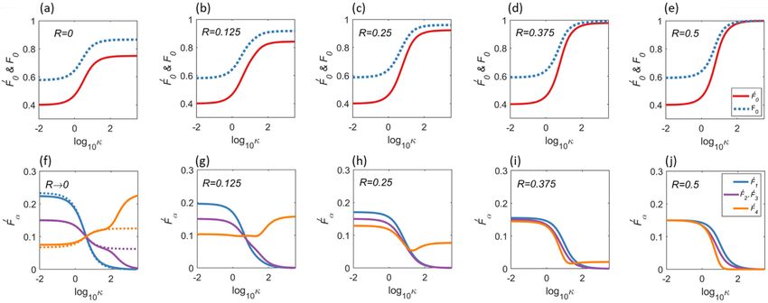
Stress-strain characterization              599

                                                                                                                                                                    Downloaded from https://academic.oup.com/gji/article/227/1/591/6293847 by guest on 27 November 2021
Figure 2. Probability density function ps (n̂) ∝ eκs(n̂) , plotted on S1 for selected values of R and κ. As κ increases, the p.d.f. becomes more localized around
the maxima of s. The projection is orthogonal to r̂2 . The p.d.f. is scaled to a maximum value of unity.

PCA basis is not the CMT mechanism, however, and the norm of its projection is not the Aki moment, though it can be very close for simple
sources.
      In our previous papers (Jordan & Juarez 2019, 2020), we instead focused on moment-oriented representations (MORs) involving the
sequential addition of basis members that best account for the low-order polynomial moments of the residual field. The mechanism that max-
imizes the zeroth-order moment is the CMT monopole (a second-order tensor), and the higher-degree terms are a source dipole (a third-order
tensor), a quadrupole (a fourth-order tensor), etc. Extending the basis by higher-moment optimization is an ill-posed orthogonalization process,
requiring heavy regularization or strong Bayesian priors (Juarez & Jordan 2020); consequently, the MOR results can be hard to interpret.
      Here we introduce an orthonormal basis set of source mechanisms that facilitates the interpretation of the moment measures of Section
3 in terms of tectonic stress and seismic strain response. We fix the zeroth-degree basis member to be the CMT mechanism M̂0 . We then
add basis members derived from rotations of M̂0 along its n̂0 , ŝ0 and b̂0 axes, and we complete the basis by including the unique mechanism
orthogonal to the other four. The projection of the moment-tensor field onto the completed orthonormal basis set constitutes what we call
the stress-oriented representation (SOR) of a moment-tensor field. The SOR recipe can be applied to any moment-tensor field, but the name
applies to the special case of an SSC field, where the expected value of the CMT mechanism always equals the reduced stress tensor.

5.1 Stress-oriented reference frame
The leading (zeroth-degree) member of the stress-oriented basis is the CMT mechanism. If the source is a realization of an SSC field, then
the expected value of its CMT mechanism is proportional to the expectation of m̂ :

       1                1
M̂0 =     Es [m̂ ] =        ps (n̂) m̂ (n̂) dn̂.                                                                                    (45)
       F0              F0
                             S1

Direct evaluation of this integral yields M̂0 = ,
                                                ˆ independent of κ. This equality also follows from the fact that M̂0 is the unique source
mechanism that maximizes the Aki moment fraction:

F0 = max ps (n̂) M̂ : m̂ (n̂) dn̂ .                                                                                                  (46)
        M̂
             S1

If M̂0 = ,
         ˆ then eq. (27) implies that
                                                   √
                                                     2
cos θ0 (n̂) = M̂0 : m̂ (n̂) =
                               ˆ : m̂ (n̂) =          s (n̂) ,                                                                                             (47)
                                                    Σ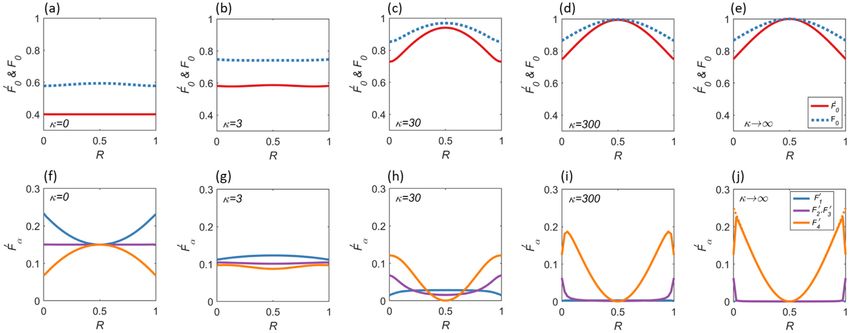
600      T.H. Jordan and A. Juarez

Figure 3. Diagonal mechanism components as functions of the differential stress ratio R. (a) DC and CLVD fractions of the CMT mechanism M̂0 . (b)
Eigenvalues of M̂0 . (c) Eigenvalues of the complementary diagonal mechanism M̂4 . These mechanisms are displayed for selected values of R in Fig. 4.

                                                                                                                                                          Downloaded from https://academic.oup.com/gji/article/227/1/591/6293847 by guest on 27 November 2021
and the Aki moment fraction becomes,
      √
        2
F0 =         eκs(n̂) s (n̂) dn̂.                                                                                                                  (48)
      NΣ
            S1

Because ps (n̂) ∝ eκs(n̂) is a strictly monotonic function of the shear traction, Es [s] maximizes Es [s  ] over all linear forms s  ∝ M̂ : m̂ ; any
rotation of M̂ away from    ˆ decreases the integral in (46).
      The CMT mechanism of an SSC field thus provides estimates of the ordered sequence of eigenvectors = (r̂1 , r̂2 , r̂3 ) and the value of
R. In this stress-oriented reference frame, it becomes

                        1               1+ R           1 − 2R             2− R
M̂0 (R) =  (R) = √ diag √
             ˆ                                    ,√              ,−√                   .                                                          (49)
                         6            1 − R + R2      1 − R + R2        1 − R + R2
This equality provides a theoretical basis for inferring tectonic stress from observed CMT mechanisms. We note that (49) holds only for
Wallace–Bott fields with images ps (n̂) on S1 that have the same symmetries as the reduced stress .
                                                                                                  ˆ The expectation of an SSC field always
has these symmetries (Fig. 2).
     A deviatoric mechanism can always be written as a linear combination of a DC and a compensated linear vector dipole (CLVD) with the
same set of principal axes (Knopoff & Randall 1970; Riedesel & Jordan 1989; Vavryčuk 2015):

M̂0 = a (R) M̂DC
              0 + b (R) M̂0
                          CLVD
                               .                                                                                                                  (50)

M̂DC
  0  is the optimal DC given by eq. (33).     0  has an r̂3 symmetry axis if R < 1/2 and an r̂1 symmetry axis if R > 1/2. The CLVD symmetry
                                            M̂CLVD
changes discontinuously at R = 1/2, where b = 0 (Riedesel & Jordan 1989):
                ⎧
                ⎪diag [1, 1, −2]       (R < 1/2)
            1 ⎨
  CLVD
M̂0     = √                                      .                                                                                     (51)
             6 ⎪⎩ diag [2, −1, −1]     (R > 1/2)
                                                               √                                                      √
The two components are not orthogonal; M̂DC      CLVD
                                           0 : M̂0    =         2
                                                                 3
                                                                     , and the normalization of (50) requires a 2 +       3ab + b2 = 1. Equating (50)
with (49) yields
         ⎧        √
         ⎪
         ⎪   √
                    3R
                           , 0 ≤ R ≤ 1/2
         ⎪
         ⎪
         ⎨ 1 − R + R2
a (R) =                                  ,                                                                                                        (52)
         ⎪
         ⎪    √
         ⎪
         ⎪       3 (R − 1)
         ⎩ √               , 1/2 ≤ R ≤ 1
               1 − R + R2

             1 − 2R
b (R) = √                 , 0 ≤ R ≤ 1.                                                                                                            (53)
            1 − R + R2
                                            (0)   (0)   (0)
The coefficients (a, b) and eigenvalues (λ1 , λ2 , λ3 ) are plotted as functions of R in Fig. 3. The DC component goes to zero as R approaches
zero ( σ1 = σ2 ) or unity ( σ2 = σ3 ) (Fig. 3), whereas the CLVD component vanishes at R = 1/2 ( σ2 = 0).

5.2 Stress-oriented basis set
Mechanism complexity is a geometrical concept describing how the elementary sources of a moment-tensor field are mis-oriented relative to
the mean mechanism M̂0 . We seek moment-valued observables that measure mechanism complexity in terms of the seismic strain response
Stress-strain characterization 601
Downloaded from https://academic.oup.com/gji/article/227/1/591/6293847 by guest on 27 November 2021
Figure 4. Stress-oriented basis sets {M̂α : α = 0, . . . , 4} for selected values of the differential stress ratio R. The CMT mechanism M̂0 (top row) and the
complementary diagonal mechanism M̂4 (bottom row) vary with R. The other three basis members (middle rows) are independent of R. The inset diagram
shows the coordinate frame. The projection is orthogonal to r̂2 .
to tectonic stress. To solve this forward problem, we construct a basis set that separates mechanism complexity into moment measures that
have clear geometrical interpretations. A physically meaningful decomposition can be achieved from the three orthogonal rotations of M̂DC 0
about its DC axes, n̂0 , ŝ0 and b̂0 . Each rotational degree of freedom generates a moment-tensor field of rank D = 2, and each of these three
fields can be represented as a linear combination of M̂0 and one other orthogonal mechanism M̂α (Jordan & Juarez 2019), which we add to
our basis set.
In the special case of zero intermediate stress, R = 1/2, the CMT mechanism is the DC,
⎡ ⎤
1 0 0
1 1 ⎢ ⎥
0 = √
M̂DC n̂0 ŝ0 + ŝ0 n̂0 = √ ⎣0 0 0⎦ (R = 1/2) . (54)
2 2 0 0 −1
The matrix components here and elsewhere are in the principal-axis frame . For visualization purposes, we take the null axis b̂0 = r̂2 to
be vertically oriented, so that M̂DC 0 represents strike-slip motion on a vertical fault plane; then, rotations about this null axis correspond to
variations in fault strike. The rotated mechanism can be expressed as a combination of M̂DC 0 and the orthogonal mechanism tensor (Jordan &
Juarez 2019),
⎡ ⎤
0 0 1
1 1 ⎢ ⎥
M̂1 = √ r̂1 r̂3 + r̂3 r̂1 = √ ⎣0 0 0⎦ . (55)
2 2 1 0 0
Similarly, the rotations of M̂DC0 about the fault normal n̂0 represent rake variations and rotations about the slip vector ŝ0 represent dip variations.
The orthogonal mechanisms that account for these two types of rotation are, respectively,
⎡ ⎤
0 1 0
1 1⎢ ⎥
M̂2 = √ n̂0 r̂2 + r̂2 n̂0 = ⎣1 0 1⎦ , (56)
2 2
0 1 0
⎡ ⎤
0 1 0
1 1⎢ ⎥
M̂3 = √ r̂2 ŝ0 + ŝ0 r̂2 = ⎣1 0 −1⎦ . (57)
2 2
0 −1 0
The four basis members (54)–(57) uniquely specify the fifth. For R = 1/2, the basis is completed by a vertically oriented CLVD,
⎡ ⎤
1 0 0
1 1 ⎢ ⎥
M̂CLVD
4 = √ r̂1 r̂1 − 2r̂2 r̂2 + r̂3 r̂3 = √ ⎣0 −2 0⎦ (R = 1/2) . (58)
6 6
0 0 1
The focal mechanisms of the R = 1/2 basis set are plotted in the middle column of Fig. 4.
In Jordan & Juarez (2020), we applied the MOR and PCA orthogonalization procedures to a single realization of the Graves &
Pitarka (2016) stochastic rupture generator and recovered basis sets that approximate the canonical basis for R = 1/2 shown in Fig. 4. This602 T.H. Jordan and A. Juarez
correspondence reflects the fact that the Graves–Pitarka model for a vertical strike-slip fault is specified in terms of strike, rake and dip
rotations. The statistical inconsistencies of the Graves–Pitarka rupture generator with the SSC model are discussed in Section 6.3.
In the general case, 0 < R < 1, the basis members can be divided into two orthogonal subspaces, the 2-D subspace of deviatoric tensors
diagonalized in the stress-oriented frame and the 3-D subspace of deviatoric tensors with all zeroes on the diagonal in this frame.
5.2.1 Diagonal moment tensors
This subspace is spanned by M̂0 = a(R) M̂DC
0 + b(R) M̂0
CLVD
and its orthogonal complement,
4 + a (R) M̂4
M̂4 (R) = b (R) M̂DC CLVD
. (59)
The coefficients a and b are given by (52) and (53). The DC component of M̂4 , like the CLVD component of M̂0 , is discontinuous at R = 1/2:
⎧
⎪diag [1, −1, 0] (R < 1/2)
1 ⎨
M̂4 = √
DC
. (60)
2 ⎪
Downloaded from https://academic.oup.com/gji/article/227/1/591/6293847 by guest on 27 November 2021
⎩diag [0, −1, 1] (R > 1/2)
The covariation of M̂0 and M̂4 with R is shown in Figs 3 and 4.
5.2.2 Off-diagonal moment tensors
For 0 < R < 1, this subspace is spanned by the basis members {M̂1 , M̂2 , M̂3 }, representing rotations of M̂DC
0 about its b̂0 , n̂0 and ŝ0 axes,
respectively. Because M̂DC
0 is fixed by the ordered reference frame , our choice of the off-diagonal basis set is independent of R. In the
degenerate cases, where two of the principal stresses are equal, M̂0 is a CLVD with either a tensional (R = 0) or compressional (R = 1)
axis of symmetry (Fig. 4), and any DC that shares this tensional or compressional axis is optimal. Hence, the off-diagonal basis set is only
defined within a rotation about the CLVD symmetry axis. This ambiguity is reflected by singularities in the high-degree (α ≥ 2) moment
measures at these limits, which are discussed in Section 5.3.
Except in the degenerate cases, the complete stress-oriented basis {M̂α : α = 0, . . . , 4} is fully determined by the CMT. This feature is
important in applications of the model because the CMTs of observed moment-tensor fields are usually well constrained by seismic data.
To represent sources with isotropic components, such as crack opening, the deviatoric basis set can be augmented with a sixth isotropic
member, M̂5 = √13 I. The SSC model assumes that any isotropic moment fraction is negligibly small.
5.3 Moment measures of an SSC field
We project the Wallace–Bott mechanism (26) onto the five basis members in Fig. 4 to obtain the direction-cosine fields:
cos θα (n̂) = M̂α : m̂ (n̂) , α = 0, . . . , 4. (61)
These basis projections are plotted on the fault-orientation sphere in Fig. 5. They display a variety of rotational and reflection symmetries that
govern the behavior of the moment integrals. Three have even parity (α = 0, 1, 4), and two have odd parity (α = 2, 3).
5.3.1 Moment measures of zeroth degree
The projections integrate to zero over the fault-orientation sphere, except the zeroth-degree term, cos θ0 (n̂), which is proportional to s(n̂) and
everywhere non-negative. The expectation of this field is the Aki moment fraction, F0 (R, κ) = Es [cos θ0 ], given by eq. (48). The expectation
of its square is the zeroth-degree fraction of the total moment,
2 2
F0 (R, κ) = E s cos θ0 = eκs(n̂;R) s 2 (n̂; R) d n̂. (62)
Σ 2 (R) N (R, κ)
S1
The R-κ maps of these moment ratios, plotted in Fig. 6, are bilaterally symmetric about the R = 1/2 midline. This bilateral symmetry,
which characterizes all of the moment measures (e.g. Fig. 7), follows from the rotational and reflection symmetries of the integrands dictated
by the SSC model. For example, s(n̂) for R = 1/2 − x equals s(n̂ ) for R = 1/2 + x because n̂ is a rotation of n̂ about the r̂2 principal axis
by an angle π/2 (Fig. 5). The integral is independent of this rigid-body rotation.
When κ = 0, the density ps is a constant on S1 , the normalization reduces to N = 4π , and F0 and F0 are proportional to spherical
averages of s(n̂) and s 2 (n̂), respectively. The square of the shear traction can be integrated analytically,
1 1
s 2 (n̂; R) d n̂ = Σ 2 (R) . (63)
4π 5
S1Stress-strain characterization 603
Downloaded from https://academic.oup.com/gji/article/227/1/591/6293847 by guest on 27 November 2021
Figure 5. Direction cosines cos θα (n̂) for Wallace–Bott mechanisms plotted in the principal-axis frame on the upper hemisphere of S1 for selected values of
R. The projection is orthogonal to r̂2 .
Figure 6. (a) Aki moment fraction F0 , (b) total-moment fraction F0 , and (c) the ratio F0 /F0 as functions of the differential stress ratio R and the logarithm of
the strain-sensitivity factor κ. (d) Variation of F0 and F0 with log k for selected values of R. (e) Variation of F0 and F0 with R for extreme values of k.
Substitution into (62) shows that F0 (R, 0) equals 2/5 independent of R, consistent with the numerical calculations in Fig. 6(e). Therefore, the
maximum mechanism complexity allowed by the SSC model is F+ = 3/5. √
In this limit of zero strain sensitivity, the Aki moment fraction is a weak function of R. It reaches a minimum value of F0 = 1/ 3 ≈ 0.577
at R = 0,1 and rises by less than 3 per cent to a maximum value of 0.593 at R = 1/2. Aki moment fractions calculated for finite-fault models604 T.H. Jordan and A. Juarez
Downloaded from https://academic.oup.com/gji/article/227/1/591/6293847 by guest on 27 November 2021
Figure 7. Expected values of the total-moment fractions F0 - F4 of an SSC field as functions of the differential stress ratio R and the strain-sensitivity factor κ,
computed using the stress-oriented basis of Fig. 4. The bottom row plots the moment measures on a linear scale for 0 ≤ κ ≤ 20; the top row plots them on a
logarithmic scale for 10−1.5 ≤ κ ≤ 103 . The plots for F2 and F3 are theoretically identical. Black lines in panels (a) and (f) are the same contours plotted in
Fig. 10.
and seismic sequences can approach this bound, implying low values of strain-sensitivity and high dispersions of fault-plane orientations
(Juarez & Jordan 2021).
F0 and F0 increase monotonically with κ, so that higher sensitivity to stress magnitude yields simpler mechanism fields. In the special
case R = 1/2, both moment measures converge asymptotically to unity (Fig. 6e), and the mechanism complexity factor F+ goes to zero. At
all other values of R, the high-κ limit of F+ is less than unity. Increasing the strain-sensitivity factor concentrates the density function around
the maximum values of the shear traction. For 0 < R < 1, these maxima occur at the four points ±n̂0 , ±ŝ0 , and the limiting form of ps is
the sum of delta functions at these points. The cases R = 0, 1 are degenerate, where the p.d.f. is delta-distributed on the two small circles at
latitudes of ±π/4 from the symmetry plane.
Owing to the exponential sharpening of the ps distribution, care must be taken in computing the expectation integral (43) for large values
of κ. Fortunately, in the asymptotic limit κ → ∞, the integrals (48) and (62) can be evaluated analytically. Owing to our stress normalization,
s0 = 1, all maxima have unit values; hence, for any 0 ≤ R ≤ 1 and any q ≥ 0,
1
lim eκs(n̂;R) s q (n̂; R) d n̂ = 1. (64)
κ→∞ N (R, κ)
S1
Applying this limit to (48) and (62), we obtain,
2 1
lim F0 (R, κ) = lim F02 (R, κ) = = . (65)
κ→∞ κ→∞ 2 (R) 1 + 43 (R − 1/2)2
These asymptotic forms satisfy eq. (17) and are well approximated by the curves computed for high κ in Fig. 6(e). They reproduce the
√
asymptotic limits along the DC midline, F0 (1/2, ∞) = F0 (1/2, ∞) = 1, as well as the values F0 (0, ∞) = 3/4 and F0 (0, ∞) = 3/4 ≈ 0.866
obtained at the corresponding CLVD extremes (R = 0, 1).
In approaching these limits, the optimal DCs given by the shear-traction maxima share a principal axis with the principal direction of
the CLVD. All optimal DCs sharing this axis have the same (optimal) projection onto this CLVD, and their zeroth-degree direction cosines
√
equal the Aki moment fraction of 3/4. In this case, the minimum complexity predicted by the SSC model is F+ (0, ∞) = 1/4 in the high-κ
limit, which compares with a maximum complexity of F+ (0, 0) = 3/5 in the low-κ limit. The non-zero value of the high-κ limit is dictated
by the SSC assumption that a CLVD CMT can only arise from a superposition of Wallace–Bott DCs and not from other source types, such
as crack-opening dipoles.Stress-strain characterization 605
Downloaded from https://academic.oup.com/gji/article/227/1/591/6293847 by guest on 27 November 2021
Figure 8. Expected values of the total-moment fractions of an SSC field as a function of log κ for selected values of R. Panels (a)–(e): zeroth-degree measures
F0 (dotted blue lines) and F0 (red lines). Panels (f)–(j): higher-degree measures Fα : α = 1−4 (coloured lines); F 2 = F 3 . Dotted lines in panel (f) show the
values for R = 0, and solid lines show the values for R = 0.01; the differences reflect the discontinuities in Fα at this limit for α = 2, 3, 4.
Figure 9. Expected values of the total-moment fractions of an SSC field as a function of R for selected values of κ. Panels (a)–(e): zeroth-degree measures
F0 (dotted blue lines) and F0 (red lines). Panels (f)–(j): higher-degree measures Fα : α = 1−4 (coloured lines); F 2 = F 3 . Dotted line in panel (j) shows
the asymptotic limit of F 4 for R > 0 (eq. 67); solid lines show the values for κ = 3000. The discontinuous behavior at R = 0, 1 reflects the limiting
discontinuities in Fα for α = 2, 3, 4.
5.3.2 Higher-degree moment fractions
The expectations of the squared direction cosines give the total-moment fractions of an SSC field as functions of R and κ,
1
Fα (R, κ) = Es cos2 θα = eκs(n̂;R) cos2 θα (n̂; R) d n̂, α = 0, . . . , 4. (66)
N
S1
These expectations are plotted in Figs 7–9. Owing to the rotational and reflection symmetries of the integrands, all of the Fα diagrams are
bilaterally symmetric about the R = 1/2 midline. The moment measures of degree 2 and 3 are identical functions of R and κ: F 2 = F 3 .
This equality holds because cos θ2 (n̂) and cos θ3 (n̂) are related by a reflection symmetry across the r̂1 -r̂2 plane. The Wallace–Bott mechanism
m̂ (n̂) is invariant with respect to this reflection, which only interchanges n̂0 and ŝ0 . These symmetries are dictated by the physics of the SSC
model.606 T.H. Jordan and A. Juarez
Table 1. Limiting values of the moment measures for the SSC model.
κ=0 κ→∞
Moment
measure R = 0, 1 R = 1/2 R = 0, 1 R → 0, 1 R = 1/2
√ √ √
F0 1/ 3 0.5935∗ 3/4 3/4 1
F0 2/5 2/5 3/4 3/4 1
F1 0.2327∗ 3/20 0 0 0
F2 3/20 3/20 1/16 0 0
F3 3/20 3/20 1/16 0 0
F4 0.0673∗ 3/20 1/8 1/4 0
∗ Computed numerically.
The R-κ maps of the moment fractions display two regimes, low-κ, and high-κ, separated by κ ≈ 3 (Fig. 7). At this value of strain
Downloaded from https://academic.oup.com/gji/article/227/1/591/6293847 by guest on 27 November 2021
sensitivity, F0 and F0 are approximately constant in R (Fig. 9b). At κ = 3, the complexity F+ is almost equipartitioned across the four
higher-degree moment fractions, which all lie within the narrow range 0.095–0.126 (Fig. 9g).
5.3.3 Low-sensitivity regime
In the low-κ regime, F0 , F 2 and F 3 are nearly constant. They are exactly constant at κ = 0, where the strain sensitivity vanishes and the
mechanism complexity factor F+ = 4α=1 Fα achieves its maximum value of 3/5. At κ = 0 and R = 1/2, the CMT is a pure DC, and the
SSC model equipartitions F+ among the non-CMT basis members: Fα = 1/4 F+ = 3/20 for α = 1, . . . , 4. Holding κ = 0 and moving
away from the midpoint, F 2 and F 3 stay constant at this value, but F 1 bows upward with R, and F 4 bows downward, such that their average
stays at 3/20. In the limits where the CMTs are pure CLVDs (R → 0 or 1), F 1 ≈ 0.233 and F 4 ≈ 0.067 (Fig 9f).
5.3.4 High-sensitivity regime
In the high-κ regime, the complexity factor F + decays monotonically as the strain sensitivity increases. Along the R = 1/2 midline, all of the
higher-degree moment fractions F α≥1 decrease monotonically as a function of κ. Their values go to zero asymptotically, as required by the
limit F 0 → 1, and their decay rates increase with degree index α. Away from the midline, the fractions F 1 - F 3 decay to zero. In the high-κ
limit, the optimal DCs are diagonal in the stress-oriented reference frame and thus completely determined by their M̂0 and M̂4 components.
The only nonzero moment fractions are F 0 and F 4 , which are related by
(R − 1/2)2
F 4 (R, ∞) := lim F 4 (R, κ) = 1 − F 0 (R, ∞) = , 0 < R < 1. (67)
κ→∞ 3/ + (R − 1/2)2
4
The domain of eq. (67) can be extended to R = 0 (and likewise to R = 1) by taking the limit F 4 (0, ∞) = lim F 4 (R, ∞). We note
R→0
that the asymptotic value of this two-variable function depends on the order in which the limits are taken, reflecting the fact that the CMT
does not define an optimal DC at R = 0, 1 for any finite κ. From eq. (67), we find F 4 (0, ∞) := lim lim F 4 (R, κ) = 1/4, whereas direct
R→0 κ→∞
computation yields lim F 4 (0, κ) = 1/8. This discontinuous decrease of F 4 at R = 0 is compensated by discontinuous increases in F 2 and
κ→∞
F 3 from 0 to 1/16, which appear as the discontinuous changes in these moment measures between R = 0 and the first positive value at 0.01
in Fig. 9j. The influence of the singularities on the three R-κ manifolds is most clearly seen in Fig. 8f, which compares the R = 0 limits
(dotted lines) with the numerically integrated values at R = 0.01 (solid lines). The two sets of curves separate at κ > 2
∼ 10 , where there is
an upward inflection in F 4 (orange curve in Fig. 8f) and a downward inflection in F 2 - F 3 (purple curve). The inflections associated with the
singularity can be tracked in Figs 8g–i to intermediate values of R.
The various limiting values of the moment fractions in both the low-sensitivity and high-sensitivity regimes are summarized in Table 1,
which gives both limiting values of the high-sensitivity regime, lim lim Fα (R, κ) and lim lim Fα (R, κ). The latter, denoted by Fα (0, ∞), is
κ→∞ R→0 R→0 κ→∞
the R → 0 limit of (67).
5.4 Mechanism complexity scale
4
The mechanism complexity of a moment-tensor field is measured by the complexity factor F+ = α=1 Fα = 1 − F0 . Contours of F+
for the SSC model are plotted as a function of R and κ in Fig. 10. The complexity is maximized at κ = 0, where F0 equals 0.4 andYou can also read