Characteristics of building fragility curves for seismic and non-seismic tsunamis: case studies of the 2018 Sunda Strait, 2018 Sulawesi-Palu, and ...
←
→
Page content transcription
If your browser does not render page correctly, please read the page content below
Nat. Hazards Earth Syst. Sci., 21, 2313–2344, 2021
https://doi.org/10.5194/nhess-21-2313-2021
© Author(s) 2021. This work is distributed under
the Creative Commons Attribution 4.0 License.

Characteristics of building fragility curves for seismic and
non-seismic tsunamis: case studies of the 2018 Sunda Strait,
2018 Sulawesi–Palu, and 2004 Indian Ocean tsunamis
Elisa Lahcene1 , Ioanna Ioannou2 , Anawat Suppasri3 , Kwanchai Pakoksung3 , Ryan Paulik4 , Syamsidik Syamsidik5 ,
Frederic Bouchette1 , and Fumihiko Imamura3
1 Geosciences   Montpellier, Montpellier University II, Montpellier, France
2 Department   of Civil, Environmental & Geomatic Engineering, University College London, United Kingdom
3 International Research Institute of Disaster Science, Tohoku University, Sendai, Japan
4 National Institute of Water and Atmospheric Research (NIWA), Wellington, New Zealand
5 Tsunami and Disaster Mitigation Research Center (TDMRC), Universitas Syiah Kuala, Banda Aceh, Indonesia

Correspondence: Elisa Lahcene (elisa.lahcene54@gmail.com) and Ioanna Ioannou (ioanna.ioannou@ucl.ac.uk)

Received: 30 November 2020 – Discussion started: 16 December 2020
Revised: 15 June 2021 – Accepted: 28 June 2021 – Published: 6 August 2021

Abstract. Indonesia has experienced several tsunamis trig-      aged prior to the tsunami’s arrival, and (iii) the buildings of
gered by seismic and non-seismic (i.e., landslides) sources.    Palu City exposed to the Sulawesi–Palu tsunami were more
These events damaged or destroyed coastal buildings and in-     susceptible to complete damage than the ones affected by the
frastructure and caused considerable loss of life. Based on     IOT, in Banda Aceh, between 0 and 2 m flow depth. Similar
the Global Earthquake Model (GEM) guidelines, this study        to the Banda Aceh case, the Sulawesi–Palu tsunami load may
assesses the empirical tsunami fragility to the buildings in-   not be the only cause of structural destruction. The build-
ventory of the 2018 Sunda Strait, 2018 Sulawesi–Palu, and       ings’ susceptibility to tsunami damage in the waterfront of
2004 Indian Ocean (Khao Lak–Phuket, Thailand) tsunamis.         Palu City could have been enhanced by liquefaction events
Fragility curves represent the impact of tsunami character-     triggered by the 2018 Sulawesi earthquake.
istics on structural components and express the likelihood
of a structure reaching or exceeding a damage state in re-
sponse to a tsunami intensity measure. The Sunda Strait and
Sulawesi–Palu tsunamis are uncommon events still poorly         1   Introduction
understood compared to the Indian Ocean tsunami (IOT), and
their post-tsunami databases include only flow depth values.    Indonesia regularly faces natural disasters such as earth-
Using the TUNAMI two-layer model, we thus reproduce the         quakes, volcanic eruptions, and tsunamis because of its geo-
flow depth, the flow velocity, and the hydrodynamic force       graphic location in a subduction zone of three tectonic plates
of these two tsunamis for the first time. The flow depth is     (Eurasian, Indo-Australian, and Pacific plates) (Marfai et al.,
found to be the best descriptor of tsunami damage for both      2008; Sutikno, 2016). The Sunda Arc extends for 6000 km
events. Accordingly, the building fragility curves for com-     from the north of Sumatra to Sumbawa Island (Lauterjung
plete damage reveal that (i) in Khao Lak–Phuket, the build-     et al., 2010) (Fig. 1a). Megathrust earthquakes regularly oc-
ings affected by the IOT sustained more damage than the         cur in this region, causing horizontal and vertical movement
Sunda Strait tsunami, characterized by shorter wave periods,    of the ocean floor which tends to be tsunamigenic (Mc-
and (ii) the buildings performed better in Khao Lak–Phuket      Closkey et al., 2008; Nalbant et al., 2005; Rastogi, 2007).
than in Banda Aceh (Indonesia). Although the IOT affected       These tsunamis are likely to cause greater destruction as they
both locations, ground motions were recorded in the city of     can follow prior damaging earthquake ground shaking and/or
Banda Aceh, and buildings could have been seismically dam-      liquefaction (Sumer et al., 2007; Sutikno, 2016). Earthquake-

Published by Copernicus Publications on behalf of the European Geosciences Union.
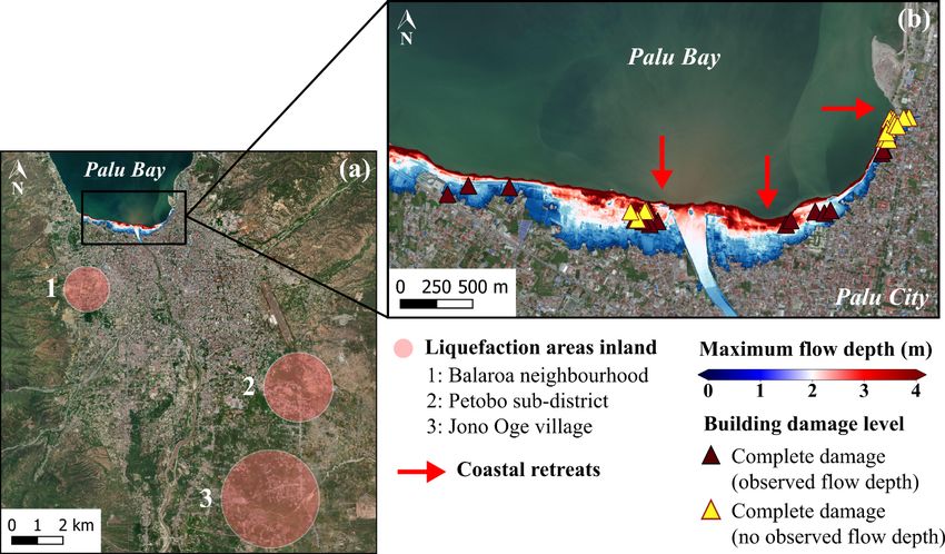
2314                    E. Lahcene et al.: Characteristics of building fragility curves for seismic and non-seismic tsunamis

Figure 1. (a) Indonesia partially surrounded by the Sunda Trench, (b) epicentre location of the 2004 Indian Ocean earthquake, (c) location of
the Sunda Strait and the Anak Krakatau volcano, and (d) epicentre location of the 2018 Sulawesi–Palu earthquake (Pakoksung et al., 2019)
and the Palu-Koro fault crossing Palu Bay, on Sulawesi Island, Indonesia (background ESRI).

generated tsunamis also tend to have longer wave periods af-             flank failure (Fig. 1c). It triggered a relatively short wave pe-
fecting the coast than non-seismic ones (Day, 2015; Grezio               riod tsunami (∼ 7 min) (Muhari et al., 2019), which devas-
et al., 2017). On 26 December 2004, the Sumatra–Andaman                  tated the western coast of Banten and the southern coast of
earthquake (Mw = 9.0–9.3) hit the north of Sumatra, In-                  Lampung with a death toll of 437 (Heidarzadeh et al., 2020;
donesia (Fig. 1b). The rupture of the seafloor is estimated              Muhari et al., 2019; National Agency for Disaster Manage-
at 1200 km length and around 200 km width (Ammon et                      ment (BNPB), 2018; Syamsidik et al., 2020). The tsunami
al., 2005; Krüger and Ohrnberger, 2005; Lay et al., 2005).               generation process is unclear. The subaerial and submarine
In the city of Banda Aceh, a strong ground shaking was                   landslide volume is still being investigated and ranges be-
recorded (Lavigne et al., 2009). This megathrust earthquake              tween 0.10 and 0.30 km3 according to recent studies (Dogan
was the second largest ever recorded (Løvholt et al., 2006)              et al., 2021; Grilli et al., 2019; Omira and Ramalho, 2020;
and caused the deadliest tsunami in the world. Overall, a                Paris et al., 2020; Williams et al., 2019). Almost 2 months
dozen Asian and African countries were devastated, with                  before this event, an unexpected tsunami struck Palu Bay, on
around 280 000 casualties (Asian Disaster Preparedness Cen-              Sulawesi Island, claiming 2000 lives and considerable loss to
ter, 2007; Suppasri et al., 2011). Although earthquakes rep-             property (Association of Southeast Asian Nations (ASEAN)-
resent the main cause of tsunamis, non-seismic events such               Coordinating Centre for Humanitarian Assistance on dis-
as landslides can also initiate tsunami waves (Grezio et al.,            aster, 2018; Omira et al., 2019). The Sulawesi earthquake
2017; Ward, 2001). After a few months of volcanic activity               (Mw = 7.5) occurred near the Palu-Koro strike-slip fault,
in the Sunda Strait, Indonesia, the Anak Krakatau volcano                50 km northwest of Palu Bay (Fig. 1d) (Socquet et al., 2019).
erupted on 22 December 2018, leading to its southwestern                 Ground shaking led to significant liquefaction along the coast

Nat. Hazards Earth Syst. Sci., 21, 2313–2344, 2021                                        https://doi.org/10.5194/nhess-21-2313-2021
E. Lahcene et al.: Characteristics of building fragility curves for seismic and non-seismic tsunamis                        2315

(Paulik et al., 2019; Sassa and Takagawa, 2019). The fault         understanding of the structural damage caused by the Sunda
mechanism did not suggest that the tsunami would be so de-         Strait and Sulawesi–Palu tsunamis and to discuss the im-
structive. The wave rapidly reached Palu (∼ 8 min), imply-         pact of wave period, ground shaking, and liquefaction events,
ing that its source was inside or near the bay (Muhari et al.,     we reproduce their tsunami intensity measures (i.e., flow
2018; Omira et al., 2019). Its short wave period (∼ 3.5 min)       depth, flow velocity, and hydrodynamic force) based on two-
also indicates a non-seismic source (i.e., landslide). Some        layer modelling (TUNAMI two-layer). We then compared
studies suggested that submarine landslides are responsible        the fragility curves of the Sunda Strait, Sulawesi–Palu, and
for the main tsunami. Moreover, a dozen coastal landslides         Indian Ocean (Khao Lak–Phuket) tsunamis to those derived
were reported during field surveys and likely contributed to       for the 2004 IOT in Banda Aceh (Indonesia), produced by
amplify tsunami waves (Arikawa et al., 2018; Muhari et al.,        Koshimura et al. (2009a). In this study, we explore the char-
2018; Omira et al., 2019; Pakoksung et al., 2019). However,        acteristics of building fragility curves for the 2018 Sunda
according to Ulrich et al. (2019), those subaerial and sub-        Strait event and 2004 IOT in Khao Lak–Phuket, as well as
marine landslides may not be the only tsunami source as the        for complex events, such as the 2018 Sulawesi–Palu tsunami
Sulawesi earthquake rupture may have also induced a large          in Palu City and the 2004 IOT in Banda Aceh, where the
portion of the tsunami waves.                                      tsunamis may not be the only cause of structural destruction.
   The term “tsunami fragility” is a measure recently pro-         Studying the impact of the wave period, ground shaking, and
posed to estimate structural damage and casualties caused          liquefaction events on the structural performance of build-
by a tsunami, as mentioned by Koshimura et al. (2009b).            ings aims to improve our knowledge on the relationship be-
Tsunami fragility curves are functions expressing the dam-         tween local vulnerability and tsunami hazard in Indonesia.
age probability of structures (or death ratio) based on the
hydrodynamic characteristics of the tsunami inundation flow
(Koshimura et al., 2009a, b). These functions have been            2     Post-tsunami databases
widely developed after tsunami events such as the 2004 In-
dian Ocean tsunami (IOT; Koshimura et al., 2009a, b; Murao         A post-tsunami database has been established for the Sunda
and Nakazato, 2010; Suppasri et al., 2011), the 2006 Java          Strait area by Syamsidik et al. (2019), Palu Bay by Paulik
tsunami (Reese et al., 2007), the 2010 Chilean tsunami (Mas        et al. (2019), and Khao Lak–Phuket by Ruangrassamee et
et al., 2012), or the 2011 great eastern Japan tsunami (Sup-       al. (2006) and Foytong and Ruangrassamee (2007) in ur-
pasri et al., 2012, 2013). Several methods aim to develop          ban areas strongly affected by these events. These databases
building fragility curves based on (i) a statistical analysis of   include 98, 371, and 120 observed flow depth traces at
on-site observations during field surveys of damage and flow       buildings, respectively. Here, the tsunami fragility analy-
depth data (empirical methods) (Suppasri et al., 2015, 2020),      sis stands on subsets of the original databases of the 2018
(ii) the interpretation of damage data from remote sensing         Sunda Strait, 2018 Sulawesi–Palu, and 2004 Indian Ocean
coupled with tsunami inundation modelling (hybrid meth-            (Khao Lak–Phuket) tsunamis, as explained in Sects. 3.2.2,
ods) (Koshimura et al., 2009a; Mas et al., 2020; Suppasri et       3.2.3, and 2.2, respectively. We define these subsets as “new”
al., 2011), or (iii) structural modelling and response simula-     databases, and we call them DB_Sunda2018, DB_Palu2008,
tions (analytical methods) (Attary et al., 2017; Macabuag et       and DB_Thailand2004, respectively. We note that the use of
al., 2014).                                                        smaller databases for the fragility assessment is expected to
   Here, we empirically developed building fragility curves        increase the uncertainty in the exact shape of the fragility
for the 2018 Sunda Strait, 2018 Sulawesi–Palu, and 2004            curves. Each database gathers exclusive information regard-
Indian Ocean (Khao Lak–Phuket, Thailand) tsunamis based            ing the degree of damage, the building characteristics, and
on the Global Earthquake Model (GEM) guidelines (Ros-              the flow depth traces (Tables 1 and 2). A brief analysis of the
setto et al., 2014). From the field surveys conducted af-          key variables (i.e., damage scale, building class, and tsunami
ter the 2018 Sunda Strait (Syamsidik et al., 2019), 2018           intensity) are presented below.
Sulawesi–Palu (Paulik et al., 2019), and 2004 Indian Ocean
(Khao Lak–Phuket, Thailand) (Foytong and Ruangrassamee,            2.1    Damage state
2007; Ruangrassamee et al., 2006) events, we utilize
three databases called DB_Sunda2018, DB_Palu2018, and              Each field survey adopted a different scale to record the de-
DB_Thailand2004, respectively. In the literature, tsunami in-      gree of structural damage. In DB_Sunda2018, the five-state
undation modelling has been performed many times to bet-           damage scale proposed by Macabuag et al. (2016) and Sup-
ter understand the tsunami hydrodynamics, especially for           pasri et al. (2020) is adopted, ranging from no damage to
earthquake-generated tsunamis (Charvet et al., 2014; Gokon         complete damage or washed away. In DB_Palu2018, the
et al., 2011; Koshimura et al., 2009a; Macabuag et al., 2016;      observed damage was classified into four states: no dam-
De Risi et al., 2017; Suppasri et al., 2011). Compared to          age, partial damage repairable, partial damage unrepairable,
the 2004 IOT, the 2018 Indonesian tsunamis are uncommon            and complete damage, as proposed by Paulik et al. (2019).
events remaining less understood. Therefore, to improve our        Finally, in DB_Thailand2004, a four-state damage scale is

https://doi.org/10.5194/nhess-21-2313-2021                                 Nat. Hazards Earth Syst. Sci., 21, 2313–2344, 2021
2316                   E. Lahcene et al.: Characteristics of building fragility curves for seismic and non-seismic tsunamis

Table 1. Harmonization between the different damage scales used in DB_Sunda2018, DB_Palu2018, and DB_Thailand2004.

             Damage state          DB_Sunda2018            DB_Palu2018                    DB_Thailand2004
             ds0                   No damage               No damage                      No damage
             ds1                   Minor damage,           Partial damage, repairable     Damage to secondary members
                                   moderate damage
             ds2                   Major damage            Partial damage, unrepairable   Damage to primary members
             ds3                   Complete damage,        Complete damage                Collapse
                                   washed away

defined by Ruangrassamee et al. (2006). To simplify the             reproduce the landslide-generated tsunami, we model the in-
comparison between the fragility curves, a harmonization of         teractions between tsunami generation and submarine land-
damage scales is proposed (Table 1). In this study, a four-         slides as upper and lower layers. The mathematical model
state damage scale ranging from ds0 to ds3 is used.                 performed in the landslide-tsunami code is obtained from
                                                                    a stratified medium with two layers. The first layer, com-
2.2     Building characteristics                                    posed of a homogeneous inviscid fluid with constant den-
                                                                    sity, ρ1 , represents the seawater, and the second layer is com-
Each survey also recorded the building construction type,           posed of a fluidized granular material with a density, ρs , and
which influences the damage probability (Suppasri et al.,           porosity, ϕ. As assumed by Macías et al. (2015), the mean
2013). In Table 2, among the 94 buildings included in               density of the fluidized sliding mass is constant and equals
DB_Sunda2018, 67 are confined masonry, 26 are timber, and           ρ2 = (1 − ϕ)ρs + ϕρ1 . We consider the two layers immisci-
1 is a steel frame building. In DB_Palu2018, most of the            ble. The governing equations are written as follows.
buildings are confined masonry with unreinforced clay bricks           The continuity equation of the seawater (first layer) is
(∼ 95 %). The database also includes reinforced concrete and
timber buildings. Finally, DB_Thailand2004 contains only            ∂Z1 ∂Q1x ∂Q1y
                                                                        +    +    = 0.                                          (1)
reinforced concrete buildings. We note that after the 2004           ∂t   ∂x   ∂y
IOT, 120 flow depth traces were recorded at reinforced con-
crete structures (e.g., residence, hotel, school, shop, bridge)       The momentum equations of the seawater in the x and
in the Khao Lak–Phuket area. As we are not considering the          y directions are
data regarding the surveyed bridges, DB_Thailand2004 in-                              !
                                                                               ∂ Q21x

cludes only 117 reinforced concrete buildings.                      ∂Q1x                   ∂ Q1x Q1y
                                                                           +            +
                                                                      ∂t      ∂x D1       ∂y   D1
2.3     Tsunami intensity                                                        ∂Z1        ∂Z2
                                                                           + gD1      + gD1     + τ1x = 0,                      (2)
                                                                                  ∂x         ∂x
The tsunami intensity has been measured in terms of flow                                             2
                                                                                                       !
                                                                                               ∂ Q1y

depth level. Table 2 also presents the number of flow depth         ∂Q1y      ∂ Q1x Q1y
                                                                           +                +
traces at surveyed buildings and the range of flow depth lev-        ∂t      ∂x      D1       ∂y D1
els for each database.                                                             ∂Z1       ∂Z2
                                                                           + gD1       + gD1     + τ1y = 0.                     (3)
                                                                                    ∂y        ∂y
3     Tsunami intensity simulations                                    The continuity equation of the landslide (second layer) is

3.1     Tsunami numerical modelling with a landslide                ∂Z2 ∂Q2x ∂Q2y
                                                                        +    +    = 0.                                          (4)
        source                                                       ∂t   ∂x   ∂y

3.1.1    Tsunami inundation model                                     The momentum equations of the landslide in the x and
                                                                    y directions are
The TUNAMI two-layer tsunami model used in the Sunda
Strait and Palu areas relies on a two-layer numerical model
solving non-linear shallow water equations. It considers two
interfacing layers and appropriate kinematic and dynamic
boundary conditions at the seafloor, interface, and water sur-
face (Imamura and Imteaz, 1995; Pakoksung et al., 2019). To

Nat. Hazards Earth Syst. Sci., 21, 2313–2344, 2021                                  https://doi.org/10.5194/nhess-21-2313-2021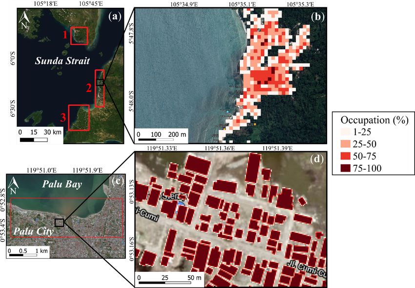
E. Lahcene et al.: Characteristics of building fragility curves for seismic and non-seismic tsunamis                               2317

Table 2. Observed flow depth traces at buildings, range of flow depth levels, and building characteristics in DB_Sunda2018, DB_Palu2018,
and DB_Thailand2004.

                                                              DB_Sunda2018               DB_Palu2018             DB_Thailand2004
  Observed flow depth traces at buildings                     94                         124                     117
  Range of observed flow depth levels at buildings (m)        (0.20, 6.60)               (0.10, 3.65)            (0.15, 10.00)
  Number of buildings per construction type                   67 confined masonry        119 confined masonry    117 reinforced
                                                              26 timber                  4 reinforced concrete   concrete
                                                              1 steel                    1 timber

                                                                         through lidar images and supplied by the Geospatial Infor-
                       !
∂Q2x    ∂       Q22x            ∂

                                        Q2x Q2y
                                                                        mation Agency (BIG), Indonesia (Fig. 2c and d).
     +                     +                                                For tsunami inundation modelling in a densely populated
 ∂t    ∂x        D2            ∂y         D2
                                                                         area, we apply a resistance law with the composite equivalent
              ∂Z2        ρ1 ∂Z1                                          roughness coefficient depending on the land use and build-
        + gD2      + gD2        + τ2x = 0,                      (5)
               ∂x        ρ2 ∂x                                           ing conditions, as shown in Eq. (8) (Aburaya and Imamura,
                                 2                                       2002; Koshimura et al., 2009a).
                                    !
                            ∂ Q2y

∂Q2y       ∂ Q2x Q2y
        +                +
 ∂t       ∂x      D2       ∂y D2                                             s
                                                                                     CD        θ
                ∂Z2       ρ1 ∂Z1                                         n = n20 +        ∗         ∗D 4/3 ,                       (8)
        + gD2       + gD2        + τ2y = 0.                     (6)                  2gd 100 − θ
                 ∂y       ρ2 ∂y
                                                                         where no corresponds to the Manning’s roughness coeffi-
   Index 1 and 2 refer to the first and the second layers, re-           cient (no = 0.025 s m−1/3 ), CD represents the drag coeffi-
spectively, and ρ1 and ρ2 are the densities of the seawater              cient (CD = 1.5; Federal Emergency Management Agency
and the landslide. Zi (x, y, t), Qi (x, y, t), and τi (x, y, t) rep-     (FEMA), 2003), and the constant d signifies the horizon-
resent the level of the layer based on the mean water level,             tal scale of buildings (∼ 15 m). θ is the building occupa-
the vertically integrated discharge, and the bottom stress in            tion ratio in percent (0 %–100 %) for each computational
each layer at each point (x, y) over the time t, respectively            cell of 20 m × 20 m and 1 m × 1 m resolutions in Sunda Strait
(Fig. A1). Di denotes the thickness of each layer. The fifth             and Palu areas, respectively. θ is obtained by computing the
term of the momentum equations (Eqs. 2, 3, 5, and 6) rep-                building area over each pixel using geographic information
resents the interaction between the two layers. The tsunami              system (GIS) data. The computational cell corresponding to
model provides the maximum water flow depth and flow ve-                 buildings can be inundated by the n Manning coefficient
locity along the coast during the tsunami inundation. The hy-            through the term D, which represents the simulated flow
drodynamic force acting on buildings and infrastructure is               depth (m). In the urban areas of Sunda Strait and Palu, the
defined as the drag force per unit width of the structure, as            average occupation ratios are 24 % and 84 %, respectively
shown in Eq. (7) (Koshimura et al., 2009b).                              (Fig. 2b and d). In non-residential areas, we set the Man-
   1                                                                     ning’s roughness coefficients inland and on the seafloor to
F = CD ρu2 D                                                    (7)      0.03 and 0.025, respectively, which are typical values for
   2
                                                                         vegetated and shallow water areas (Kotani, 1998).
CD represents the drag coefficient (CD = 1.0 for simplicity),
ρ is the seawater density (ρ = 1000 kg m−3 ), u stands for the           3.2     Calibration and validation of the tsunami
current velocity (m s−1 ), and D is the inundation depth (m).                    inundation model

3.1.2   Flow resistance within a tsunami inundation area                 3.2.1    Performance parameters

BATNAS and DEMNAS, Indonesia, provided the bathymet-                     The tsunami inundation model is calibrated using two per-
ric and topographic data at 180 and 8 m resolutions, respec-             formances parameters: K and κ proposed by AIDA (1978),
tively. The data were established from synthetic aperture                as defined below:
radar (SAR) images (http://tides.big.go.id/DEMNAS/index.                               n
                                                                                    1X
html, last access: 2 February 2020). Both datasets were re-              log K =          log Ki ,                                  (9)
sampled to three computational domains with a grid size                             n i=1
of 20 m resolution (Fig. 2a and b). In Palu City, the bathy-
metric and topographic data at 1 m resolution were obtained

https://doi.org/10.5194/nhess-21-2313-2021                                        Nat. Hazards Earth Syst. Sci., 21, 2313–2344, 2021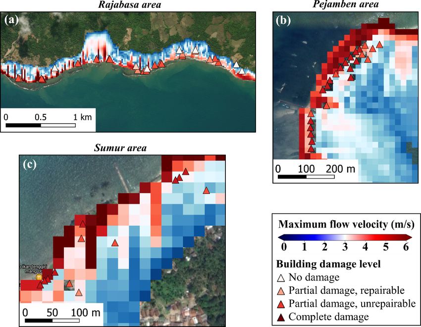
2318                   E. Lahcene et al.: Characteristics of building fragility curves for seismic and non-seismic tsunamis

Figure 2. (a and c) Computational areas in the Sunda Strait (1–3) and Palu City, and (b and d) magnified view of the building occupation
ratio in Sunda Strait (20 m resolution) and Palu City (1 m resolution) (background ESRI and © Google Maps).

        v
        u n                                                           as follows: ρ2 = 1500 kg m−3 , α = 5◦ , and VS = 0.15 km3 .
        u1 X
log κ = t       (log Ki )2 − (log K)2 ,                     (10)      We reach the best fit between the simulated and observed
          n i=1                                                       flow depths at buildings for 10 min sliding time. Never-
        xi                                                            theless, most of the simulated flow depths are underesti-
Ki =       ,                                                (11)      mated compared to the observed ones, with a mean differ-
        yi
                                                                      ence of 0.28 ± 1 m. Using quantum GIS (QGIS) software,
where xi and yi are the recorded and simulated tsunami flow           we smoothed the 1st DEM to remove these mean differences
depths at location i. K is defined as the geometrical mean            in elevation at buildings where the flow depth is underesti-
of Ki , and κ is defined as deviation or variance from K.             mated. The resulting DEM (2nd DEM) provides a topogra-
The Japan Society of Civil Engineers (JSCE) (2002) recom-             phy more reliable at buildings (Fig. 3). We completed three
mends 0.95 < K < 1.05 and κ < 1.45 for the model results              cross sections along the Sunda Strait coasts to show the dif-
to achieve “good agreement” in the tsunami source model               ferent corrections applied to the DSM (Fig. 4a–g). K and
and propagation and inundation model evaluation (Otake et             κ values for damaged buildings are 0.99 and 1.11, respec-
al., 2020; Pakoksung et al., 2018).                                   tively, which means that we achieve “good agreement” for
                                                                      the Sunda Strait tsunami model, displayed in Fig. 5a–f. We
3.2.2    The 2018 Sunda Strait tsunami inundation model               note that the simulated inundation zone overlays 94 build-
                                                                      ings out of 98. In Sect. 4.1, the Sunda Strait tsunami fragility
To correct the digital surface model (DSM), we removed the            assessment is based on these 94 buildings (DB_Sunda2018).
vegetation, building, and infrastructure elevations based on          Simulation snapshots of the Sunda Strait tsunami propaga-
the linear smoothing method and used the resulting digital            tion are shown in Fig. B1 10, 20, 60, and 120 s after the
elevation model (1st DEM) as topography in the tsunami in-            tsunami generation. In Fig. B2, the simulated tsunami height
undation model (Fig. 3). The vertical accuracy of the DSM             based on the best-fitting parameters is also displayed. Fig-
and DEM is about 4 m. The 2018 Sunda Strait tsunami model             ure B3 illustrates the maximum simulated flow velocity of
depends on the density of the landslide (ρ2 ), its stable slope       the 2018 Sunda Strait tsunami inundation model.
(α), its volume (VL ), and its sliding time (tS ). As proposed
by Paris et al. (2020), the low sensitivity parameters are set

Nat. Hazards Earth Syst. Sci., 21, 2313–2344, 2021                                    https://doi.org/10.5194/nhess-21-2313-2021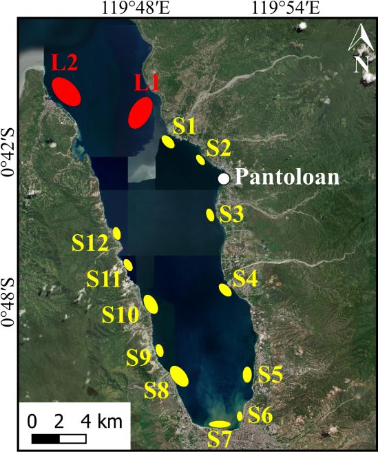
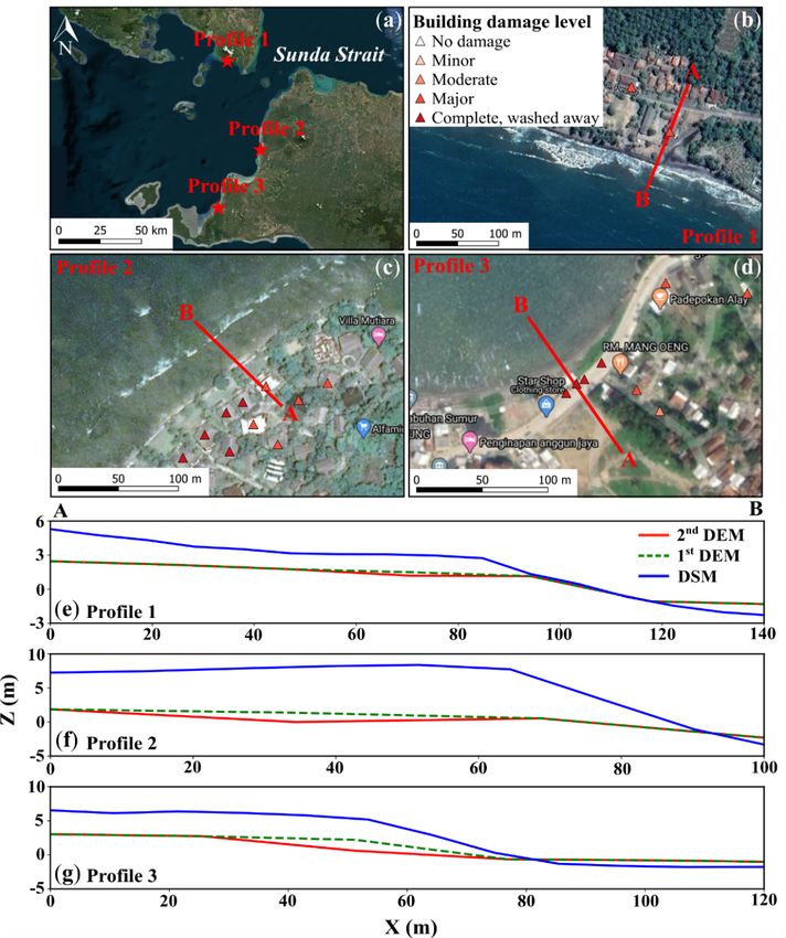
E. Lahcene et al.: Characteristics of building fragility curves for seismic and non-seismic tsunamis                                       2319

Figure 3. Topographic corrections performed on the DSM and the 1st DEM. The 2nd DEM is used as new topography in the TUNAMI
two-layer model.

Figure 4. (a) Cross sections along Sunda Strait coasts. One cross section is realized in the computational areas (b and e) 1, (c and f) 2, and (d
and g) 3 to illustrate the topographic corrections applied to the DSM at buildings using QGIS (a triangle represents a building) (background
ESRI and © Google Maps).

https://doi.org/10.5194/nhess-21-2313-2021                                         Nat. Hazards Earth Syst. Sci., 21, 2313–2344, 2021
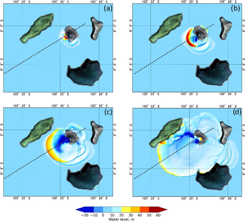
2320                   E. Lahcene et al.: Characteristics of building fragility curves for seismic and non-seismic tsunamis

Figure 5. (a, c, and e) Sunda Strait final tsunami inundation model with the maximum simulated flow depth overlaid on the damaged building
data in the computational areas 1 to 3, and (b, d, and f) magnified views of the maximum simulated flow depth in the Rajabasa, Pejamben,
and Sumur areas (background ESRI and © Google Maps).

Nat. Hazards Earth Syst. Sci., 21, 2313–2344, 2021                                      https://doi.org/10.5194/nhess-21-2313-2021
E. Lahcene et al.: Characteristics of building fragility curves for seismic and non-seismic tsunamis                                            2321

Table 3. Hypothesized landslide parameters (location and volume)                     City; the slide direction, captured by an aircraft pilot, is
in Palu Bay.                                                                         perpendicular to the bay (Carvajal et al., 2019). The den-
                                                                                     sity of the landslides (ρ2 ), their stable slope (α), and their
    No.        Location (latitude; longitude)              Volume (106 m3 )          sliding time (ts ) are set as follows: ρ2 = 2000 kg m−3 (Palu
    L1a                        −0.655; 119.749                          37.54
                                                                                     Bay receives a large amount of fine continental deposits
    L2a                        −0.670; 119.801                          31.93        such as clay-sized sediments; Frederik et al., 2019), α = 14◦
    S1b                        −0.680; 119.821                           0.60        (Chakrabarti, 2005), and tS = 10 min. For a landslide ratio
    S2b                        −0.703; 119.842                           0.18        of 1.2 (i.e., S8 volume is multiplied by 1.2), the tsunami
    S3b                        −0.737; 119.851                           0.25        model shows a great similarity between observed and sim-
    S4b                        −0.789; 119.862                           0.75        ulated flow depths (a = 1.027). The simulated tsunami in-
    S5b                        −0.852; 119.878                           0.22        undation zone overlays 175 traces out of 371 because (i)
    S6b                        −0.879; 119.871                           0.60        151 buildings with flow depth traces are not included in our
    S7b                        −0.885; 119.858                           2.44        computational area (Fig. 2c) and (ii) 45 buildings are out-
    S8b                        −0.846; 119.822                           4.45        side the simulated tsunami envelope, which is shorter than
    S9b                        −0.832; 119.813                           0.83        the surveyed one (Fig. 8). The geometric mean is near the
    S10b                       −0.804; 119.808                           2.17        recommended values (K = 0.93), while the standard devia-
    S11b                       −0.774; 119.792                           0.55        tion and the root mean square error (RMSE) are high (κ =
    S12b                       −0.754; 119.788                           0.83        2.18, RMSE = 0.92 m). Therefore, to develop accurate and
  a Based on our assumption from Arikawa et al. (2018) and Heidarzadeh et al.        reliable curves, we set a 1 m confidence interval including
  (2019). b Based on observations from satellite imagery, field surveys, and video   124 flow depth traces at buildings out of 175 (Fig. 9). In
  footage (Arikawa et al., 2018; Carvajal et al., 2019).                             Sect. 4.2, the Sulawesi–Palu tsunami fragility assessment is
                                                                                     based on these 124 buildings (DB_Palu2018). K and κ val-
                                                                                     ues for damaged buildings are 0.93 and 2.14, respectively,
3.2.3     The 2018 Sulawesi–Palu tsunami inundation                                  with a root mean square error of 0.26 m. The validity of the
          model                                                                      model is mainly based on the geometric mean K, close to
                                                                                     0.95, so we consider the tsunami inundation model accu-
We increased the mean sea level (MSL) by 2.3 m to repro-                             rate enough (Fig. 8). In Fig. C1, the simulation snapshots of
duce the high tide during the 2018 Sulawesi–Palu tsunami.                            the Sulawesi–Palu tsunami propagation are shown 2, 10, 30,
As shown by Pakoksung et al. (2019), the observed wave-                              and 60 s after the tsunami generation. The simulated tsunami
form at Pantoloan tidal gauge does not fit the simulated one                         height based on the best-fitting parameters is also displayed
with the finite fault model of TUNAMI-N2. Although recent                            in Fig. C2. Figure C3 illustrates the maximum simulated
studies show that seismic seafloor deformation may be the                            flow velocity of the 2018 Sulawesi–Palu tsunami inundation
primary cause of the tsunami (Gusman et al., 2019; Ulrich et                         model.
al., 2019), in this study, the main assumption is that the 2018
Sulawesi–Palu event was triggered by subaerial and subma-
rine landslides. According to Heidarzadeh et al. (2019), a                           4   Tsunami fragility assessment
large landslide to the north or the south of Pantoloan tidal
gauge is responsible for the significant height wave recorded.                       The proposed fragility assessment framework has two main
Arikawa et al. (2018) also identified several sites of poten-                        steps. In the first step, an exploratory analysis aims to (i) as-
tial subsidence in the northern part of Palu Bay. Based on                           sess the trends that the available data follow and (ii) deter-
these previous studies, we assume two large landslides: L1                           mine the main explanatory variables that need to be included
and L2. Small landslides (S1–S12) also occurred in the bay;                          in the statistical model and their influence on the slope and
their location is known from observations from satellite im-                         intercept of the fragility curves. Then, we select a statistical
agery, field surveys, and video footage (Arikawa et al., 2018;                       model and examine its goodness-of-fit to the data based on
Carvajal et al., 2019) (Fig. 6). From the trial and error method                     the observations of the exploratory analysis. We note that the
and the topographic and bathymetric data provided by the                             development of the computed fragility curves for the 2018
Geospatial Information Agency (BIG), we determined the                               Sunda Strait and 2018 Sulawesi–Palu tsunamis is directly
soil property and achieved the volume of the landslides (Ta-                         based on DB_Sunda2018 and DB_Palu2018, in which each
ble 3). In Fig. 7, the submarine landslides model reproduces                         building has both observed and simulated flow depth values
well the tsunami observations at Pantoloan.                                          (Table 4).
   The calibration of the model depends on the landslide                                To explore the relationship between the tsunami intensity
S8 because (i) as a small landslide, its volume is too small                         and the probability of damage, we fit a generalized linear
to distort the simulated wave height at the Pantoloan tidal                          model (GLM) to the data of each database, as proposed by
gauge, (ii) it has the largest volume among the other small                          the GEM guidelines (Rossetto et al., 2014). A GLM assumes
landslides, and (iii) it is close and ideally oriented to Palu                       that the response variable yij is assigned 1 if the building

https://doi.org/10.5194/nhess-21-2313-2021                                                  Nat. Hazards Earth Syst. Sci., 21, 2313–2344, 2021
2322                    E. Lahcene et al.: Characteristics of building fragility curves for seismic and non-seismic tsunamis

Table 4. Number of buildings used for the tsunami fragility analysis of the 2018 Sunda Strait, 2018 Sulawesi–Palu, and 2004 IOT (Khao
Lak–Phuket) events.

                  Database                                                     Tsunami intensity measure
                                             Observed flow          Simulated flow          Simulated flow         Simulated hydrodynamic
                                                     depth                   depth                velocity                           force
                  DB_Sunda2018a                             94                      94                      94                                    94
                  DB_Palu2018b                             124                     124                     124                                   124
                  DB_Thailand2004                          117                       –                       –                                     –
                a Surveyed buildings included in the Sunda Strait simulated tsunami inundation zone. b Surveyed buildings included in the Palu
                simulated tsunami inundation zone and in the 1 m confidence interval.

                                                                                        j sustained damage DS ≥ dsi and 0 otherwise. The variable
                                                                                        follows a Bernoulli distribution:

                                                                                        yij ∼ Bernoulli (πi (x̃j )),                                   (12)

                                                                                        where πi (x̃j ) is the probability that a building j will reach or
                                                                                        exceed the “true” damage state dsi given estimated tsunami
                                                                                        intensity level x̃j . The Bernoulli distribution is characterized
                                                                                        by its mean,

                                                                                        µij = πi (x̃j ),                                               (13)

                                                                                        which is expressed here in terms of a probit model, com-
                                                                                        monly used to express the mean in the empirical fragility
                                                                                        assessment field (Rossetto et al., 2013), defined in terms of
                                                                                        8[.], the cumulative distribution function of a standard nor-
                                                                                        mal distribution:

                                                                                        8−1 [πi (x̃j )] = ηij ,                                        (14)

                                                                                        where ηij is the linear predictor, which can be written in the
                                                                                        form
Figure 6. Location of the hypothesized landslides (S: small; L:
large) in Palu Bay (background ESRI).                                                   ηij = θ0i + θ1i ln(x̃j ),                                      (15)

                                                                                        where θ1i and θ0i are the two regression coefficients rep-
                                                                                        resenting the slope and the intercept, respectively, of the
                                                                                        fragility curve corresponding to damage state dsi . For the ex-
                                                                                        ploratory analysis, the tsunami intensity is measured in terms
                                                                                        of observed flow depth levels. We also fit the GLM models
                                                                                        to subsets of data of each database to explore the importance
                                                                                        of the construction type to the shape of the fragility curves.
                                                                                        The confidence in the exact shape of the mean curves is es-
                                                                                        timated and presented in terms of the 90 % confidence inter-
                                                                                        vals around the best-estimate curves.
                                                                                           Based on the aforementioned observations, we construct
                                                                                        parametric statistical models for the three databases to (i)
                                                                                        identify the simulated tsunami measure type that fits the data
                                                                                        best and (ii) construct fragility curves for the tsunami inten-
                                                                                        sity type that fits the data best.
Figure 7. Comparison between observed and simulated wave                                   Ideally, the response variable yij of an appropriate statis-
heights at Pantoloan tidal gauge in Palu Bay, Sulawesi, Indonesia.                      tical model is the damage state i = {0, 1, 2, 3} sustained by
                                                                                        a building j . The damage state follows a categorical distri-
                                                                                        bution (i.e. also called a generalized Bernoulli distribution)

Nat. Hazards Earth Syst. Sci., 21, 2313–2344, 2021                                                         https://doi.org/10.5194/nhess-21-2313-2021
E. Lahcene et al.: Characteristics of building fragility curves for seismic and non-seismic tsunamis 2323
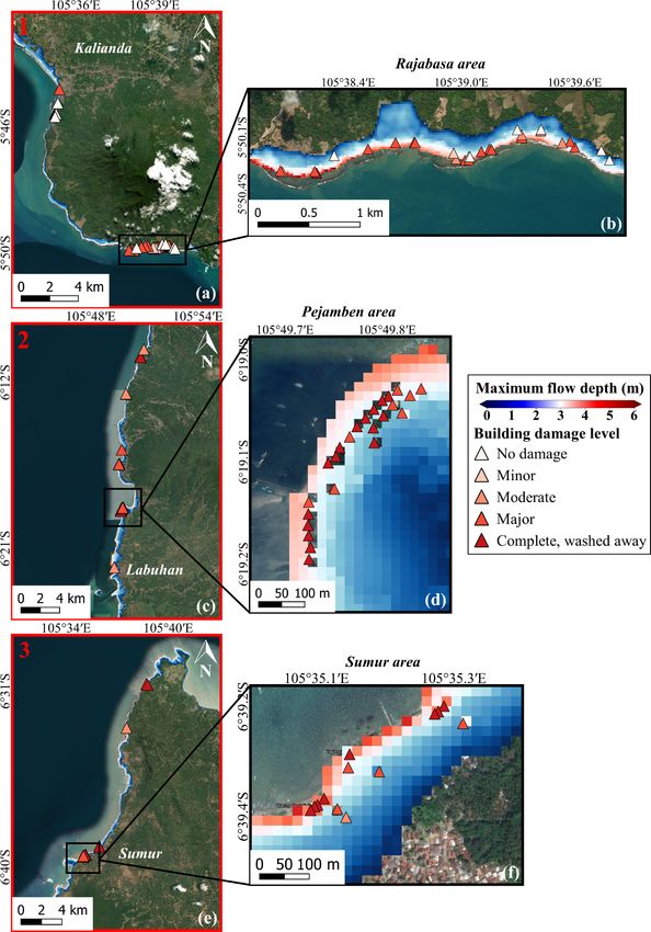
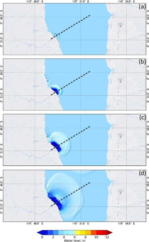
Figure 8. Sulawesi–Palu final tsunami inundation model with the maximum simulated flow depth overlaid on the damaged building data
(background ESRI).
2013), namely the logit and complementary loglog (termed
here “cloglog”), are considered in the form
−1
8 πi x̃j , probit
πi (x̃j )
ηij = ln 1−π x̃ , logit . (18)
i( j )
ln − ln 1 − πi x̃j , cloglog
The linear predictor is also expressed in various forms of in-
creasing complexity, as depicted in Eq. (19).
θ0 + θ1 x̃j
(19a)
θ 0 + θ 1i x̃ j (19b)
ηij = θ0 + θ1 x̃j + θ2 class (19c)
θ0 + θ1i x̃j + θ2 class
(19d)
θ0 + θ1 x̃j + θ2 class + θ3 x̃j class (19e)
Figure 9. Comparison between observed and simulated flow depths
at damaged building for an S8 ratio of 1.2; a confidence interval is Class is a categorical unordered variable which expresses
set at 1 m flow depth. here the construction type. θ0−3 are the unknown regression
coefficients of the model. Equations (19a) and (19b) assume
that the fragility curves are only influenced by the tsunami in-
which describes the possible levels of damage i = {0, 1, 2, 3} tensity. Equation (19a) assumes that the slope of the fragility
sustained by a given building (Table 1). The random compo- curves is the same for all damage states. In contrast, Eq. (19b)
nent of this model can be written as allows the slope of each curve to vary for each damage state;
yij ∼ Categorical (P (DS = dsi x̃j )), (16) the slope varies for each fragility curve. The following three
equations account for the influence of the building class (i.e.
where P (DS = dsi x̃j ) is the probability that a building the construction type) in the shape of the fragility curves.
j will reach the “true” damage state dsi given estimated All three equations assume that the construction type affects
tsunami intensity level x̃j . the intercept of the fragility curves, and only Eq. (19e) as-
sumes that the construction type affects both the intercept
and the slope of the curves. Finally, Eqs. (19c) and (19e) as-
1 − πi x̃j ,
i=0
sume identical slopes for all fragility curves irrespective of
P (DS = dsi x̃j ) = πi x̃j − πi+1 x̃j , 0 < i < imax the damage state. In contrast, Eq. (19d) relaxes this assump-
πi x̃j , i = imax
tion and considers that the slope changes for each damage
(17) state. The combinations of random and systematic compo-
nents result in five distinct models (Table 5).
Multiple expressions of the systematic component are con- In what follows, we fit multiple models to each database
structed to test their goodness of fit. With regard to the based on the observations of the exploratory analysis. We ex-
link function, apart from the commonly used probit func- amine the goodness of fit of these models for a given tsunami
tion, two alternative expressions found in the GEM guide- intensity measure and link function with two formal tests,
lines for empirical vulnerability assessment (Rossetto et al., as proposed in the GEM guidelines (Rossetto et al., 2014).
https://doi.org/10.5194/nhess-21-2313-2021 Nat. Hazards Earth Syst. Sci., 21, 2313–2344, 20212324 E. Lahcene et al.: Characteristics of building fragility curves for seismic and non-seismic tsunamis
Table 5. Statistical models examined for each database. fragility curves are constructed using bootstrap analysis. Ac-
cording to the latter analysis, 1000 samples of the database
Model Component are obtained with a replacement, and the selected model is
Random Systematic refitted to each sample.
M1 Eq. (19a) 4.1 DB_Sunda2018
M2 Eq. (19b)
M3 Eq. (16) Eq. (19c)
M4 Eq. (19d)
We fit the GLM models to the data in DB_Sunda2018 (ir-
M5 Eq. (19e) respective of their structural characteristics), and we plot
the obtained probit functions against the natural logarithm
of the observed flow depth to explore how the slope and
the intercept of the models change for each damage state
(Fig. 10a). The 90 % confidence intervals around the best-
estimate curves are also included. All three curves have posi-
tive slopes, which indicates that the flow depth is an adequate
descriptor of the damage caused by a tsunami as the prob-
ability of a given damage state being reached or exceeded
increases with the increase in the flow depth. The slope of
each function is similar for ds2 and ds3 and different for ds1 .
Nonetheless, the curve corresponding to ds1 is also associ-
ated with substantial uncertainty. In Fig. 10b, we fit probit
models to subsets of the available data for the two main con-
struction types. One of the drawbacks of the small database
is that not all damage states were observed for each building
class. Therefore, the comparison of probit models is limited
for damage states ds2 and ds3. The curves for the two con-
struction types appear to be substantially different. As ex-
pected, the timber buildings are more vulnerable than the
confined masonry buildings. Their intercept is responsible
for the difference as the two curves are parallel. It indicates
the need to develop a statistical model which allows only the
intercept to change with the construction type, and the slope
should be identical.
Following the main observations of the exploratory anal-
ysis, we consider that M3 is an acceptable model with two
Figure 10. Probit functions fitted for each individual damage state explanatory variables: the tsunami intensity and the construc-
to DB_Sunda2018 (a) to assess whether the observed flow depth tion type. To assess its goodness of fit, we consider each link
is an efficient descriptor of damage and (b) to assess whether the function with three alternatives for the linear predictor (i.e.,
construction type affected the shape of fragility curves for ds2 and M4, M5, and M1) which relax some of its assumptions. In
ds3 . In both cases, the 90 % confidence interval is plotted. Table 6, we compare the AIC values of the three models to
assess the fit of the different models for the observed flow
depth levels assuming the probit link function. M3 has the
Firstly, we compare the Akaike information criterion (AIC) smallest AIC value compared to its alternatives, which indi-
values, which estimates the prediction error of the examined cates that it fits the data better than the remaining three mod-
models (Akaike, 1974). The model with the lowest value fits els. Nonetheless, some of these differences are rather small,
the data best. The alternative models used in this study are and it raises the question of whether the improvement in the
nested, which means that the more complex model includes fit provided by M3 is statistically significant over its alterna-
all the terms of the simpler ones plus an additional term. For tives. To address this, we perform likelihood ratio tests, and
this reason, we also perform a series of likelihood ratio tests the results are reported in Table 7. We note that the p values
to examine whether the fit provided by the model with the vary for the three comparisons. The p value is significantly
lowest AIC value is statistically significant over its alterna- above the 0.05 threshold when the identical slope for each
tive nested models, which relaxes its assumptions (Rossetto fragility curve assumption (i.e. comparison of M3 and M4)
et al., 2014). We also use the AIC value to determine which is tested. This means that M4 (which assumes varying slopes
of these simulated intensity measures fits the data best. Fur- for each damage state) does not provide a statistically sig-
thermore, the 90 % confidence intervals of the best-estimate nificant improvement than its alternative. Therefore, the fit
Nat. Hazards Earth Syst. Sci., 21, 2313–2344, 2021 https://doi.org/10.5194/nhess-21-2313-2021E. Lahcene et al.: Characteristics of building fragility curves for seismic and non-seismic tsunamis 2325
Table 6. AIC values for the three models assuming probit link func- Table 7. Likelihood ratio test summary for all available observed
tion fitted to the observed and simulated tsunami intensity measures and simulated tsunami intensity measures of DB_Sunda2018.
of DB_Sunda2018.
Model p value
Model AIC
Observed Simulated Simulated Simulated
Observed Simulated Simulated Simulated flow flow flow hydrodynamic
flow flow flow hydrodynamic depth depth velocity force
depth depth velocity force
M3 ∼ 0.41 ∼ 0.72 ∼ 0.08 ∼ 0.05
M3 129.9 138.5 224.2 194.9 M4
M4 137.7 148.4 227.7 210.3 M3 ∼ 0.56 ∼ 0.39 ∼ 0.36 ∼ 0.35
M5 131.6 139.8 225.3 196.1 M5
M1 162.0 169.0 246.5 216.9 M3 ∼ 0.00 ∼ 0.00 ∼ 0.00 ∼ 0.00
M1
of M3 is the best. Similarly, the p value is well above the Table 8. AIC values for model M1 fitted to the simulated tsunami
threshold for M3 vs. M5, highlighting that the construction intensity measures of DB_Palu2018.
type does not affect the slope of the fragility curves. In con-
trast, the p value is well below the threshold for the com- Link Model AIC
parison of M3 and M1, indicating that the construction type function
is an important variable and affects only the intercept. Hav-
Simulated Simulated Simulated
ing concluded that M3 based on the observed flow depth data
flow flow hydrodynamic
fits the data better than its alternatives (i.e. M4, M5, and M1), depth velocity force
we repeat the procedure to identify which simulated intensity
type fits the data best. Table 6 also shows the comparison probit M1 276.8 286.3 283.3
of the AIC values for the three simulated tsunami intensity logit M1 276.2 286.3 283.1
cloglog M1 280.3 286.5 284.7
types. For all simulated intensity types, M3 is identified as
the model which fits the data better than its alternatives, and
this conclusion is further reinforced by the likelihood ratio
tests presented in Table 7. By comparing the AIC values for 4.2 DB_Palu2018
M3 for all three simulated intensity types, we note that the
simulated flow depth is the tsunami intensity that fits the data We also fit GLM models to the data in DB_Palu2018 using
best. The aforementioned observations can also be made if the observed tsunami flow depth to express the tsunami in-
instead of the probit link function, the two alternative func- tensity and then to construct fragility curves and their 90 %
tions (i.e. logit and cloglog) are considered, as depicted in confidence intervals for the three individual damage states
Table D1. The comparison of the AIC values of M3 for the (Fig. 11). The data seem to produce fragility curves with pos-
three link functions identifies the probit link function as the itive slopes for dS1 and dS2 and a negative slope for dS3 . This
one that fits the data best. latter observation is counter-intuitive as it is expected that
The regression coefficients of the 2018 Sunda Strait the likelihood of collapse will grow with the increase in the
fragility curves based on the best-fitted M3 model with a pro- tsunami depth. This outcome could be attributed to the col-
bit link function are listed in Table E1. An advantage of con- lected sample, which includes very few collapsed buildings
structing a complex model that accounts for the ordinal na- observed at low flow depth levels.
ture of the damage and for the two main construction types Based on the observations of the exploratory analysis,
in the systematic component is that fragility curves for tim- we use identical slopes for the fragility curves for all three
ber buildings can be obtained even for the states for which damage states (ds1 − ds3 ) to tackle the negative slope for
there are available data. A timber building is found to sus- ds3 and three link functions. Therefore, model M1 is fitted
tain more damage than confined masonry buildings for the to DB_Palu2018 assuming that the tsunami intensity is ex-
more intense damage states. Nonetheless, there is substan- pressed in terms of simulated flow depth, flow velocity, and
tially more uncertainty in the prediction of the likelihood of hydrodynamic force. Table 8 depicts the AIC values for each
damage, and this can be attributed to the rather small sample model. We note that for all cases the flow depth fits the data
size. the best. Table 8 also shows that the logit function fits the
data best. The regression coefficients of the 2018 Sulawesi–
Palu fragility curves for the logit function are depicted in Ta-
ble E2.
https://doi.org/10.5194/nhess-21-2313-2021 Nat. Hazards Earth Syst. Sci., 21, 2313–2344, 20212326 E. Lahcene et al.: Characteristics of building fragility curves for seismic and non-seismic tsunamis
Table 9. AIC values for the two models fitted to the observed flow layer model (Figs. 13a and 14a). For instance, when the ob-
depth of DB_Thailand2004. served and simulated flow depths reach 3 m, the likelihood of
minor to major damage (i.e., ≥ ds1 , ds2 ) for both timber and
Model AIC confined masonry buildings is approximately 99 % (Fig. 14a
Observed flow depth and b). In contrast, the likelihood of complete damage (i.e.,
≥ ds3 ) is 70 % for timber buildings and only 10 % for con-
Link function probit logit cloglog fined masonry buildings. Consequently, the tsunami func-
M1 264.3 262.4 263.5 tions based on observation and simulation are highly simi-
M2 267.8 266.3 265.3
lar, which illustrates the accuracy and the reliability of the
tsunami inundation model. The curves show that confined
masonry-type buildings have higher performance than tim-
4.3 DB_Thailand2004 ber structures. When the flow depth is greater than 5 m and
2.5 m, the probability of complete damage is around 99 %
The exploratory analysis aims to identify trends in the shape for confined masonry and timber buildings, respectively.
of the fragility curves for each damage state. Thus, we We also compare the completely damaged or washed away
fit GLM models to DB_Thailand2004 to construct fragility fragility curve for confined-masonry buildings to Syamsidik
curves for the three individual damage states, and we plot et al. (2020), who developed the curve as a function of ob-
them with their 90 % confidence interval in Fig. 12. The served flow depth for these buildings, as depicted in Fig. 13a.
data seem to produce fragility curves with positive slopes for Fragility curves representing complete damage or washed
all three damage states and also are parallel to each other, away are similar up to 4.5 m flow depth. Each curve es-
which suggests that the slope should be identical for all three timates a 15 % building damage probability at 3.5 m flow
curves. depth. However, a few data points are available beyond 5 m
Based on the observations of the exploratory analysis, we in the Sunda Strait area. Therefore, the damage probability
consider model M1 as the most suitable. To test its goodness uncertainty is greater for this value, hence the difference be-
of fit, model M2, which relaxes the assumption that the slope tween our ds3 -curve and the one produced by Syamsidik et
of all three curves is identical, is also fitted to the data. In al. (2020). The curves as functions of the maximum simu-
Table 9, the comparison of the AIC values for the two models lated flow velocity and the hydrodynamic force are displayed
also shows that M1 is the model which fits the data best for in Figs. 13b and 14b and Figs. 13c and 14c for confined ma-
all three link functions considered in this study (i.e., probit, sonry concrete and timber buildings, respectively.
logit, and cloglog). We also perform a likelihood ratio test to
confirm that the improvement in the fit provided by the more 5.2 Building fragility curves of the 2018 Sulawesi–Palu
complex M2 model over M1 is not statistically significant. tsunami
The p value is found to be equal to 0.76, 0.95, and 0.33 for
the probit, logit, and cloglog functions, respectively, which is The 2018 Sulawesi–Palu tsunami curves are developed for
significantly above the 0.05 threshold. This suggests that M2 confined masonry buildings with unreinforced clay brick of
does not provide a statistically better fit to the data; therefore, DB_Palu2018. The computed and surveyed curves show a
the less complex M1 model fits the data best. The regression similar damage trend. When the observed and simulated flow
coefficients of the 2004 Indian Ocean (Khao Lak–Phuket) depths reach 1.5 m, the building damage probabilities for
fragility curves for the best-fitted model M1 with logit link partial damage repairable (i.e., ≥ ds1 ), partial damage un-
function can be found in Table E3. repairable (i.e., ≥ ds2 ), and complete damage (i.e., ≥ ds3 )
are around 90 %, 40 %, and 15 %, respectively (Fig. 15a).
5 Results The fragility curves based on the observed and simulated
flow depths are relatively similar, especially for ds1 and ds3 .
5.1 Building fragility curves of the 2018 Sunda Strait The curves based on the flow velocity and the hydrodynamic
tsunami force are displayed in Fig. 15b and c.
The fragility curves determine conditional damage proba- 5.3 Comparison between the 2018 and 2004 building
bilities according to the tsunami intensity measures of the fragility curves
2018 Sunda Strait event for both confined masonry con-
crete (Fig. 13a–c) and timber (Fig. 14a–c) buildings of In Fig. 16, we compare (i) the Sunda Strait and Sulawesi–
DB_Sunda2018. In Fig. 14a and b, there are no data to pre- Palu ds3 -curves based on the simulated tsunami intensity
dict the shape of the curves between 0–1 m flow depth and measures for confined masonry-type buildings, (ii) the 2004
0–1 m s−1 flow velocity. The curves as a function of the ob- Indian Ocean (Khao Lak–Phuket, Thailand) ds3 -curve based
served flow depth reveal a great similarity with the ones on the observed flow depth for reinforced-concrete infilled
based on the simulated flow depth from the TUNAMI two- frames buildings (Foytong and Ruangrassamee, 2007; Ros-
Nat. Hazards Earth Syst. Sci., 21, 2313–2344, 2021 https://doi.org/10.5194/nhess-21-2313-2021E. Lahcene et al.: Characteristics of building fragility curves for seismic and non-seismic tsunamis 2327 Figure 11. Probit functions fitted for each individual damage state to DB_Palu2018 to assess whether the observed flow depth is an efficient descriptor of damage. The 90 % confidence interval is plotted. Figure 12. Probit functions fitted for each individual damage state to DB_Thailand2004 to assess whether the observed flow depth is an efficient descriptor of damage. The 90 % confidence interval is plotted. https://doi.org/10.5194/nhess-21-2313-2021 Nat. Hazards Earth Syst. Sci., 21, 2313–2344, 2021
2328                   E. Lahcene et al.: Characteristics of building fragility curves for seismic and non-seismic tsunamis

Figure 13. The 2018 Sunda Strait curves for confined masonry concrete buildings. Best-estimate fragility curves, with their 90 % confidence
intervals, as functions of (a) the observed and the maximum simulated flow depths, (b) the maximum simulated flow velocity, and (c) the
simulated hydrodynamic force for confined masonry concrete buildings of DB_Sunda2018 sustaining minor or moderate damage (ds1 ),
major damage (ds2 ), and complete damage or washed away (ds3 ) in Sunda Strait area.

setto et al., 2007; Ruangrassamee et al., 2006), and (iii) the          velocity attains 6 m s−1 , the curve estimates 99 % building
2004 Indian Ocean (Banda Aceh, Indonesia) ds3 -curves pro-              damage probability in Banda Aceh. The hydrodynamic force
duced by Koshimura et al. (2009a). The curves are based on              also contributes to increase the probability of complete dam-
a visual damage interpretation of remaining roofs using the             age in Banda Aceh. For example, when the force reaches
pre- and post-tsunami satellite data (IKONOS) and are thus              25 kN m−1 , the damage probability is around 99 % in Banda
developed for mixed buildings (low-rise wooden, timber-                 Aceh (Fig. 16c, Table 10).
framed, and non-engineered reinforced concrete construc-
tions; Koshimura et al., 2009a; Saatcioglu et al., 2006). For
1 m flow depth, the likelihood of complete damage is greater            6     Discussion
in Palu (10 %) than in Banda Aceh, Khao Lak–Phuket, and
Sunda Strait (Fig. 16a, Table 10). However, when the flow               6.1    Reliability of the building fragility curves
depth reaches 3 m, the damage probability is about 50 % in
Banda Aceh, 25 % in Palu City, and less than 20 % in Khao               The reliability of the curves depends mainly on (i) the qual-
Lak–Phuket. We also note that the likelihood of completely              ity and the quantity of post-tsunami data and (ii) whether
damaged or washed away buildings is higher in Sunda Strait              the tsunami intensity measures are efficient predictors of
than in Khao Lak–Phuket above 4 m flow depth. However,                  damage. With regard to the first factor, DB_Sunda2018,
the data points in Thailand are mostly ranging from 0 to                DB_Palu2018, and DB_Thailand2004 include relatively lit-
5 m, and the 90 % confidence interval upon this value is con-           tle data (Table 2). For each database, the relatively broad
stantly increasing with the flow depth. Below 1 m s−1 , the             confidence intervals around the best-estimate fragility curves
flow velocity has a low impact on the damage probability in             reflect the small sample size. Moreover, the complexity of
Banda Aceh (< 1 %). However, beyond this value, the prob-               each studied event also plays a role in how well the selected
ability of damage becomes very sensitive to the current ve-             tsunami intensity measure can represent the tsunami dam-
locity (Fig. 16b, Table 10). As an example, when the flow               age. In particular, in DB_Sunda2018 and DB_Thailand2004,
                                                                        only the tsunami load is responsible for the building dam-

Nat. Hazards Earth Syst. Sci., 21, 2313–2344, 2021                                      https://doi.org/10.5194/nhess-21-2313-2021
E. Lahcene et al.: Characteristics of building fragility curves for seismic and non-seismic tsunamis 2329
Figure 14. The 2018 Sunda Strait curves for timber buildings. Best-estimate fragility curves, with their 90 % confidence intervals, as functions
of (a) the observed and the maximum simulated flow depths, (b) the maximum simulated flow velocity, and (c) the simulated hydrodynamic
force for timber buildings of DB_Sunda2018 sustaining minor or moderate damage (ds1 ), major damage (ds2 ), and complete damage or
washed away (ds3 ) in Sunda Strait area.
age. In contrast, in DB_Palu2018, buildings may have suf- measure. In Sunda Strait, the DEM resolution is relatively
fered prior damage due to ground shaking and liquefaction high (20 m), and it could explain why the flow velocity is not
(Kijewski-Correa and Robertson, 2018; Sassa and Takagawa, a good descriptor of damage. In Palu City, we perform two-
2019). Nonetheless, we are not able to establish precisely layer numerical modelling using the finest grid size of 1 m.
which of the surveyed buildings had suffered prior damage in However, the 2018 Palu tsunami is a complex event. The sub-
the database and to what extent. The complexity of the 2018 aerial and submarine landslides may not be the main cause of
Sulawesi–Palu event could introduce a bias in the tsunami the tsunami, as shown by Ulrich et al. (2019), and this could
fragility assessment, and this has also been mentioned for have affected the flow velocity data. As the flow velocity of
other events such as the 2011 great eastern Japan tsunami the Sunda Strait and Sulawesi–Palu tsunamis does not pro-
(Charvet et al., 2014). This bias could explain why we ob- vide a good description of the damage, we cannot evaluate
served a negative slope for our ds3 -curves based on the ob- the impact of floating debris on Indonesian structures (Song
served flow depth combined with very few collapsed build- et al., 2017). The hydrodynamic force of these events, com-
ings, especially for very low intensity levels (Fig. 11). De- puted from the flow velocity and the flow depth, does not
spite the aforementioned reservations, the adopted statistical provide a good description of the tsunami damage either.
tests identified that the flow depth is consistently the best de-
scriptor of the tsunami damage for both the DB_Sunda2018
6.2 Impact of the wave period, ground shaking, and
and DB_Palu2018 data, while the flow velocity is the worst.
liquefaction events on the building damage
This finding is in line with similar observations made by
probability
Macabuag et al. (2016). De Risi et al. (2017) illustrated well
the influence of the DEM resolution and the model sources
on the efficiency of the flow velocity as a tsunami intensity The curve comparison illustrates well the relationship be-
tween the 2004 Indian Ocean, the 2018 Sunda Strait, and the
https://doi.org/10.5194/nhess-21-2313-2021 Nat. Hazards Earth Syst. Sci., 21, 2313–2344, 2021You can also read