Article - American Meteorological ...
←
→
Page content transcription
If your browser does not render page correctly, please read the page content below
Article
SOUTHTRAC-GW
An Airborne Field Campaign to Explore Gravity Wave
Dynamics at the World’s Strongest Hotspot
Markus Rapp, Bernd Kaifler, Andreas Dörnbrack, Sonja Gisinger,
Tyler Mixa, Robert Reichert, Natalie Kaifler, Stefanie Knobloch,
Ramona Eckert, Norman Wildmann, Andreas Giez, Lukas Krasauskas,
Peter Preusse, Markus Geldenhuys, Martin Riese, Wolfgang Woiwode,
Felix Friedl-Vallon, Björn-Martin Sinnhuber, Alejandro de la Torre,
Peter Alexander, Jose Luis Hormaechea, Diego Janches,
Markus Garhammer, Jorge L. Chau, J. Federico Conte,
Peter Hoor, and Andreas Engel

                                  ABSTRACT: The southern part of South America and the Antarctic peninsula are known as the
                                  world’s strongest hotspot region of stratospheric gravity wave (GW) activity. Large tropospheric
                                  winds are deflected by the Andes and the Antarctic Peninsula and excite GWs that might propagate
                                  into the upper mesosphere. Satellite observations show large stratospheric GW activity above
                                  the mountains, the Drake Passage, and in a belt centered along 60°S. This scientifically highly
                                  interesting region for studying GW dynamics was the focus of the Southern Hemisphere Transport,
                                  Dynamics, and Chemistry–Gravity Waves (SOUTHTRAC-GW) mission. The German High Altitude
                                  and Long Range Research Aircraft (HALO) was deployed to Rio Grande at the southern tip of
                                  Argentina in September 2019. Seven dedicated research flights with a typical length of 7,000 km
                                  were conducted to collect GW observations with the novel Airborne Lidar for Middle Atmosphere
                                  research (ALIMA) instrument and the Gimballed Limb Observer for Radiance Imaging of the
                                  Atmosphere (GLORIA) limb sounder. While ALIMA measures temperatures in the altitude range
                                  from 20 to 90 km, GLORIA observations allow characterization of temperatures and trace gas
                                  mixing ratios from 5 to 15 km. Wave perturbations are derived by subtracting suitable mean
                                  profiles. This paper summarizes the motivations and objectives of the SOUTHTRAC-GW mission.
                                  The evolution of the atmospheric conditions is documented including the effect of the extraordi-
                                  nary Southern Hemisphere sudden stratospheric warming (SSW) that occurred in early September
                                  2019. Moreover, outstanding initial results of the GW observation and plans for future work are
                                  presented.

                                  KEYWORDS: Dynamics; Gravity waves; Mountain waves; Stratospheric circulation;
                                  Aircraft observations

https://doi.org/10.1175/BAMS-D-20-0034.1
Corresponding author: Markus Rapp, markus.rapp@dlr.de
In final form 23 November 2020
©2021 American Meteorological Society
For information regarding reuse of this content and general copyright information, consult the AMS Copyright Policy.
              This article is licensed under a Creative Commons Attribution 4.0 license.

                AMERICAN METEOROLOGICAL SOCIETY
                                                                                                                   Unauthenticated      021    E871
                                                                                                                           A P R I L| 2Downloaded 09/23/21 03:30 AM UTC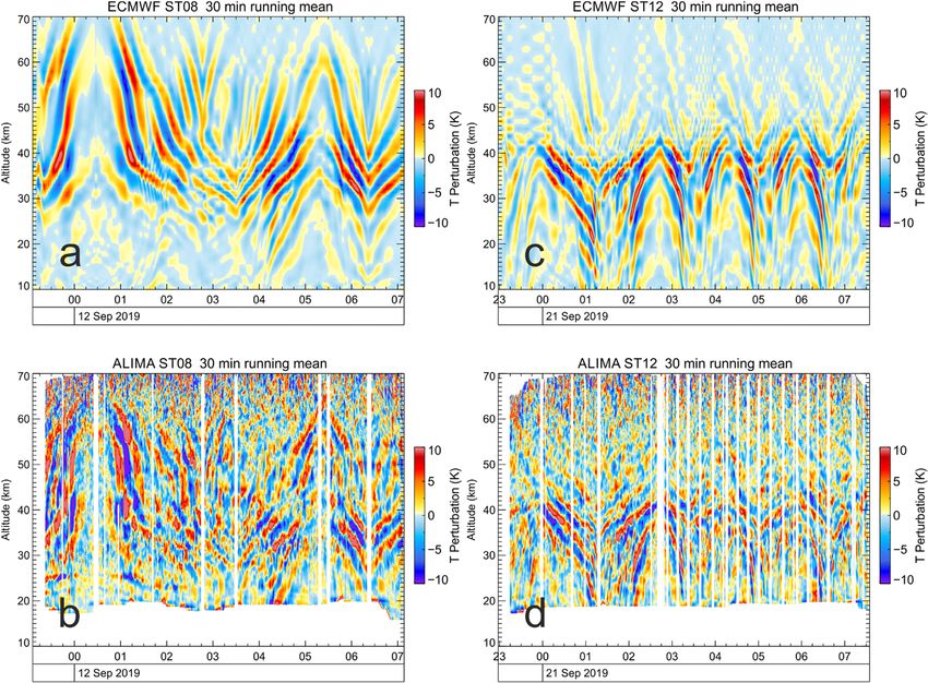
AFFILIATIONS: Rapp—Institut für Physik der Atmosphäre, Deutsches Zentrum für Luft- und Raumfahrt,
Oberpfaffenhofen, and Meteorologisches Institut München, Ludwig-Maximilians-Universität
München, Munich, Germany; Kaifler, Dörnbrack, Gisinger, Mixa, Reichert, Kaifler, Knobloch, Eckert, and
Wildmann—Institut für Physik der Atmosphäre, Deutsches Zentrum für Luft- und Raumfahrt, Oberpfaffen-
hofen, Germany; Giez—Einrichtung Flugexperimente, Deutsches Zentrum für Luft- und Raumfahrt,
Oberpfaffenhofen, Germany; Krasauskas, Preusse, Geldenhuys, and Riese—Institute of Energy and
Climate Research (IEK-7), Forschungszentrum Jülich, Jülich, Germany; Woiwode, Friedl-Vallon, and
Sinnhuber—Institute of Meteorology and Climate Research, Karlsruhe Institute of Technology, Karlsruhe,
Germany; de la Torre—Facultad de Ingeniería, Universidad Austral, LIDTUA (CIC), and CONICET, Pilar,
Argentina; Alexander—IFIBA, CONICET, Buenos Aires, Argentina; Hormaechea—Estación Astrónomicas
Río Grande, Facultad de Ciencias Astronómicas y Geofísicas, Universidad Nacional de La Plata, and
CONICET, La Plata, Argentina; Janches—NASA Goddard Space Flight Center, Greenbelt, Maryland;
Garhammer—Meteorologisches Institut München, Ludwig-Maximilians-Universität München, Munich,
Germany; Chau and Conte—Leibniz Institute of Atmospheric Physics, Kühlungsborn, Germany; Hoor—
Institute of Atmospheric Physics, Johannes Gutenberg University of Mainz, Mainz, Germany; Engel—
Institute for Atmospheric and Environmental Sciences, Goethe University Frankfurt, Frankfurt, Germany
T
he region of the southern Andes and the Antarctic Peninsula is known as the world’s
strongest stratospheric hotspot of gravity wave (GW) activity (in terms of strength and
occurrence frequency) occurring during austral winter and lasting to early spring (e.g.,
Hoffmann et al. 2013; P. Alexander et al. 2010; de la Torre et al. 2012; Llamedo et al. 2019).
Known sources of GWs are flow over orography [in which case the GWs are called mountain
waves (MWs)], convection, and spontaneous emission (Fritts and Alexander 2003;
Plougonven and Zhang 2014). While intense MW activity is expected above and in the lee
of the mountains given the prevailing strong tropospheric westerly winds, it is, however,
somewhat surprising that strong GW activity is observed in the middle to upper stratosphere
along 60°S spinning from the Drake Passage to the South Pacific (see, e.g., Ern et al. 2006;
M. J. Alexander et al. 2010; Hindley et al. 2015; and Fig. 1 for illustration). This circumpolar
Fig. 1. Illustration of the GW belt based on ERA5 temperature perturbations for (left) August
—–———–—–
and (right) September 2019 at a pressure levels of 10 hPa. Shown is |T | = √(T639 – T106 )2 (K; see
“Models” section for details). The red oval marks the target area where airborne measurements
were conducted during SOUTHTRAC-GW.
AMERICAN METEOROLOGICAL SOCIETY
Unauthenticated 021 E872
A P R I L| 2Downloaded 09/23/21 03:30 AM UTC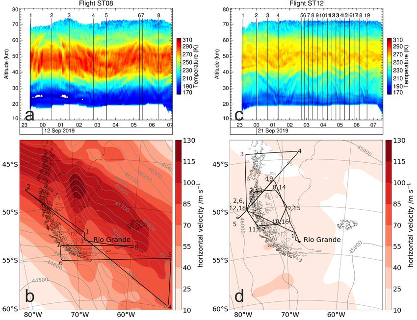
band of almost zonally symmetric GW activity and related momentum fluxes will be referred
to as the “gravity wave belt.”
   While observational evidence for the GW belt is undisputed, state of the art climate mod-
els fail to reproduce this feature with important consequences (McLandress et al. 2012;
Geller et al. 2013). The “missing drag at 60°S” in the models leads to a too strong polar night
jet (PNJ) and hence to too low temperatures in the southern polar winter stratosphere known
as the “cold pole bias” of climate models affecting the polar stratospheric cloud formation and
heterogeneous ozone chemistry [Butchart et al. 2011; Stratosphere–Troposphere Processes and
Their Role in Climate (SPARC); SPARC 2010]. In addition, the breakdown of the polar vortex is
simulated to occur too late in spring leading to a lagged recovery of the Antarctic ozone hole
(Austin et al. 2003; McLandress and Shepherd 2009). McLandress et al. (2012) showed that
adding artificial MW drag along 60°S in a numerical experiment resulted in more realistic
stratospheric winds and higher polar temperatures. In the same spirit, Garcia et al. (2017)
enhanced the orographic GW (OGW) forcing in the SH by simply doubling the magnitude
of sources to achieve more realistic climatologies of tropospheric and stratospheric winds,
temperatures, and ozone concentrations. However, they also showed that a parameterization
for non-OGWs (NOGW) leads to similar improvements of wind and temperature climatologies.
Thus, OGWs play an important role, but also NOGW sources likely contribute to the “missing
drag at 60°S” (see also Cámara et al. 2016; Holt et al. 2017).
   Accordingly, several different physical processes, involving both OGW and NOGW, have
been proposed to account for the observed belt of enhanced stratospheric GW momentum
fluxes around 60°S: These are 1) downwind advection and meridional refraction of OGW
from the southern Andes and the Antarctic Peninsula into the PNJ (Dunkerton 1984;
Preusse et al. 2002; Sato et al. 2009, 2012); 2) unresolved OGWs from small islands
(Alexander and Grimsdell 2013; Alexander et al. 2009; Vosper 2015; Pautet et al. 2016;
Eckermann et al. 2016); 3) the generation of secondary waves in the breaking regions
of these primary orographic waves (Satomura and Sato 1999; Hindley et al. 2015); 4)
NOGWs from sources associated with winter storm tracks over the Southern Ocean
(Wu and Eckermann 2008; Hendricks et al. 2014; Plougonven et al. 2015) or with convec-
tion and frontogenesis (Choi and Chun 2013; Holt et al. 2017); 5) and finally, a zonally
uniform distribution of small amplitude waves from nonorographic mechanisms such as
spontaneous adjustment and jet instability around the edge of the stratospheric PNJ
(Sato and Yoshiki 2008; Hindley et al. 2015, 2019).
   It is hence obvious that the Southern Hemisphere region around 60°S is a scientifically
highly interesting target for studying GW processes and their impact on the stratospheric cir-
culation and climate. Already in the austral winter of 2014 the Deep Propagating Gravity Wave
Experiment (DEEPWAVE) conducted research flights with two aircraft from Christchurch,
New Zealand, and involved various ground based instruments, satellite datasets, as well as a
variety of numerical models of different complexity (Fritts et al. 2016). DEEPWAVE was also the
first comprehensive airborne mission studying GW dynamics up to the mesopause (~100 km).
To mention just a few outstanding results, DEEPWAVE provided insight into the relation
between tropospheric forcing and GW activity in the middle atmosphere (Fritts et al. 2016,
2018; Kaifler et al. 2015; Bramberger et al. 2017; Portele et al. 2018), the horizontal propaga-
tion of OGW into the polar night jet (Ehard et al. 2017), secondary wave generation in regions
of strong MW breaking (Bossert et al. 2017), the effect of the background atmosphere on
GW propagation also in the absence of critical level filtering (Kruse et al. 2016), the relative
contribution of various parts of the GW spectrum to momentum fluxes (Smith et al. 2016;
Smith and Kruse 2017, 2018; Bossert et al. 2018), and the general characteristics of both
OGWs and NOGWs (Smith et al. 2016; Smith and Kruse 2017; Eckermann et al. 2016;
Pautet et al. 2016, 2019; Jiang et al. 2019).

AMERICAN METEOROLOGICAL SOCIETY
                                                                       Unauthenticated      021    E873
                                                                               A P R I L| 2Downloaded 09/23/21 03:30 AM UTC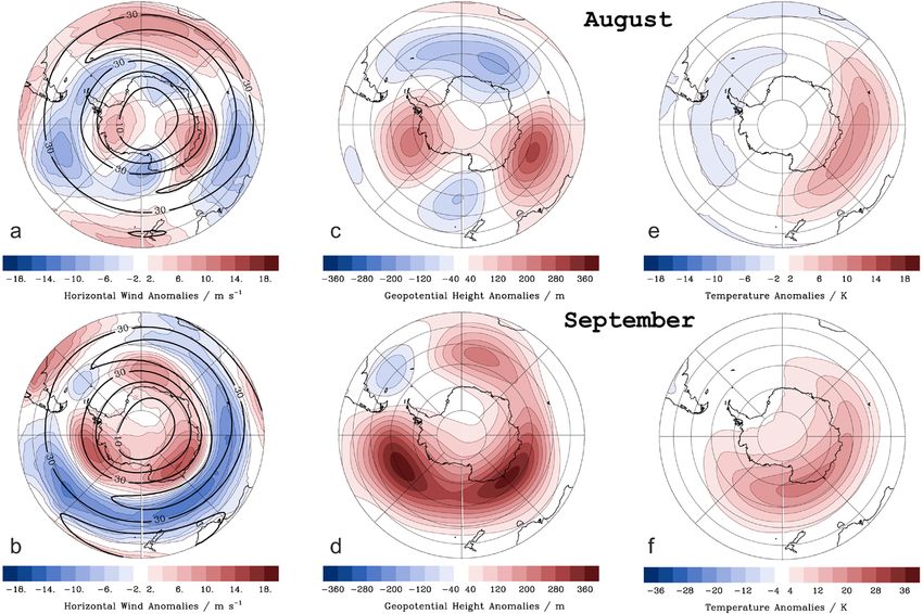
DEEPWAVE explored mainly GWs over the Southern Alps at about 45°S and only few flights
went down to latitudes south of 55°S (Fig. 2 of Pautet et al. 2019). As a complementary ex-
periment to DEEPWAVE and targeting the Southern Hemisphere GW hotspot, the Southern
Hemisphere Transport, Dynamics, and Chemistry–Gravity Waves (SOUTHTRAC-GW) airborne
research mission with the
German High Altitude and
Long Range Research Aircraft
(HALO) was conducted from
Rio Grande, Tierra del Fuego,
Argentina (53°S, 67°W), as
part of the more comprehen-
sive SOU T H T R AC mission
(see www.pa.op.dlr.de/southtrac
/science/scientific-objectives/). The
objectives of SOUTHTRAC-GW
are summarized in Table 1.
    In the second section, we de-
scribe the research aircraft and
its instruments dedicated to the
measurements of GW proper-
ties, along with the ground           Fig. 2. (a) Group photo of the campaign participants of the SOUTHTRAC-
based measurements in the             GW mission in front of the HALO aircraft inside the hangar of the naval
region. We will introduce the         air base in Rio Grande. (b) HALO aircraft outside the hangar of the naval
forecast model tools used for         air base in Rio Grande during a test run of the ALIMA instrument with its
flight planning as well as re-        green laser beam pointing upward. (c) DLR scientist Norman Wildmann
                                      mounting a 5-hole probe to measure meteorological parameters on the
analysis fields which are being
                                      Stemme aircraft of glider pilot Klaus Ohlmann. (d) Impressive MW cloud
used for the interpretation of        over the southern Andes as seen during a flight of the Stemme.
atmospheric measurements. In
the third section, we describe
the prevailing meteorological conditions under which the flights were conducted. Mission
overview and initial promising results are presented in the fourth section. The article closes
with a summary and outlook on ongoing and planned analysis work in the fifth section.

Instruments and datasets
HALO and airborne instruments. The German research aircraft HALO is based on a Gulfstream
G550 business jet with a maximum range of ~8,000 km, a maximum flight altitude of ~15 km,
and a typical cruise speed of ~800 km h−1 (cf. Fig. 2, upper- and lower-left panels). It has been
modified to allow gas sampling and optical experiments in the cabin and to mount several

Table 1. Scientific objectives of SOUTHTRAC-GW.

 No.                                                       Objective
 1       Yield coordinated observations in the troposphere, stratosphere, and mesosphere for the early propagation of
         OGWs excited over the southern Andes and/or Antarctic Peninsula into the PNJ
 2       Better quantify the mountain waves in the vicinity of their sources and document the early stages of their
         vertical and horizontal propagation
 3       Provide unprecedentedly detailed measurements for comparison and validation of high-resolution simulations
         that can resolve, in case studies, much of the GW spectrum
 4       Explore the breaking and dissipation of the GWs, including the excitation of secondary GW
 5       Compare the identification of GW as seen by different measurement techniques

AMERICAN METEOROLOGICAL SOCIETY
                                                                                          Unauthenticated      021    E874
                                                                                                  A P R I L| 2Downloaded 09/23/21 03:30 AM UTC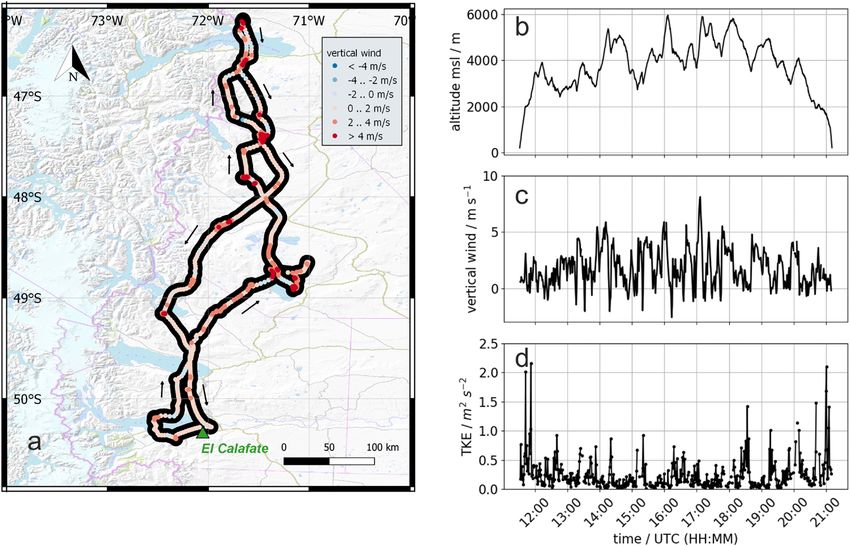
spectrometers under the wings as well as a “belly pod” under its fuselage to carry large
instruments (Krautstrunk and Giez 2012). In total, HALO may carry up to three tons of sci-
entific payload. HALO has been in service since 2012 and has by now been used in scientific
missions addressing a broad spectrum of atmospheric chemistry and physics research objec-
tives (e.g., Wendisch et al. 2016; Voigt et al. 2017; Schäfler et al. 2018; Stevens et al. 2019;
Oelhaf et al. 2020).
   During SOUTHTRAC-GW there were three prime instruments dedicated to the measure-
ments of GW signatures, namely, the novel Airborne Lidar for Middle Atmosphere research
(ALIMA), the Gimballed Limb Observer for Radiance Imaging of the Atmosphere (GLORIA),
and the Basic HALO Measurement and Sensor System (BAHAMAS).
   As deployed during SOUTHTRAC-GW, ALIMA is a compact upward pointing Rayleigh
lidar using a pulsed neodymium-doped yttrium aluminum garnet (Nd:YAG) laser transmit-
ting 12.5 W (125 mJ) at 532 nm with a 48-cm diameter receiving telescope, and using three
height-cascaded elastic detector channels to yield atmospheric density profiles in the altitude
range from 20 to 90 km. Density profiles are converted to temperatures using hydrostatic
downward integration (Hauchecorne and Chanin 1980). For typical horizontal and vertical
integration intervals of 10 and 1 km, respectively, temperatures are derived between 20- and
80-km altitude. From 20 to 60 km the corresponding error is 0.9 K, from 60 to 70 km it is
2.9 K, and above it is 6.5 K. From 20 to 60 km the error is near constant because the signal
is distributed over the three height-cascaded detector channels. To separate GW-induced
temperature perturbations from atmospheric background temperatures a 30-min running
mean (corresponding to a flight distance of ~400 km) is applied.
   The infrared limb imager GLORIA performs two-dimensional and tomographic
measurements of temperatures and trace gas mixing ratios (Friedl-Vallon et al. 2014;
Riese et al. 2014). For this purpose, GLORIA combines a Michelson interferometer with
a 2D infrared detector and measures molecular thermal emissions in the spectral range
between 780 and 1,400 cm−1 (7.1–12.8 μm). GLORIA is mounted in the belly pod. Its line
of sight aims toward the horizon on the right side of the aircraft and measures infrared
radiation emitted by molecules in the atmosphere. The horizontal observation angle is
varied from 45° to 135° with respect to the flight direction. In this way, the instrument can
investigate the same air volume from different directions, which allows for a tomographic
retrieval scheme (Ungermann et al. 2011; Kaufmann et al. 2015; Krisch et al. 2018). In the
vertical, GLORIA may sample the atmosphere from ~1 km above cruise altitude down to
approximately 5-km altitude (below which the investigated spectral lines become optically
thick). GLORIA was applied under different measurement strategies to the observation of
GW (Krisch et al. 2017, 2020). GW effects on the distribution of trace gases were investigated
by Woiwode et al. (2018) and Kunkel et al. (2019).
   While GLORIA and ALIMA enable characterization of the atmosphere below and above
the aircraft, respectively, the BAHAMAS system consists of a nose tip probe with a 5-hole
wind sensor and yields in situ measurements of horizontal and vertical winds along
with temperatures and pressures at flight level at high temporal resolution, i.e., of up to
100 Hz (Giez et al. 2017, 2019). Corresponding data have been successfully used for the
derivation of momentum and energy fluxes owing to GW as well as for turbulence analysis
(Bramberger et al. 2017; Portele et al. 2018; Bramberger et al. 2020; Gisinger et al. 2020;
Wilms et al. 2020).
   Finally, besides HALO a Stemme S10VT motor glider (cf. Fig. 2, upper-right panel) was
also deployed to the nearby city of El Calafate (cf. Fig. 8) and equipped with another 5-hole
probe to measure temperature and wind distributions in the MWs over the southern Andes
(see Fig. 2, lower-right panel, for a photo taken from the cockpit of the Stemme during one of
the glider flights).

AMERICAN METEOROLOGICAL SOCIETY
                                                                       Unauthenticated      021    E875
                                                                               A P R I L| 2Downloaded 09/23/21 03:30 AM UTC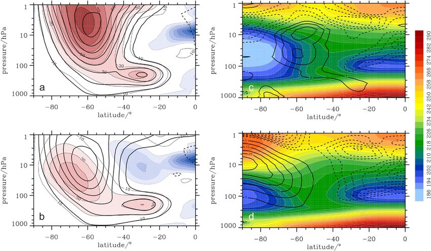
Ground-based and satellite instruments and radiosondes. The Estación Astrónomicas
Río Grande (EARG), which is located close to the airport of Rio Grande, hosts a number of
ground based instruments that were useful as supplementary observations to the airborne
measurements. For SOUTHTRAC-GW the Compact Rayleigh Autonomous Lidar (CORAL)
(Kaifler and Kaifler 2020; Reichert et al. 2019) and the Southern Argentina Agile Meteor
Radar (SAAMER) (Fritts et al. 2010b) provided important background information on middle
atmosphere temperature, winds, and momentum fluxes, respectively.
   CORAL measures atmospheric density from roughly 15–90-km altitude. The Rayleigh
lidar emits 12-W power at 532-nm wavelength and receives backscattered photons with
a 63-cm diameter telescope using three height-cascaded elastic detector channels and
one Raman channel. As in the case of ALIMA, density profiles measured with CORAL
are converted to temperature profiles using hydrostatic downward integration. CORAL is
a portable lidar and commenced operation at EARG in November 2017. CORAL operates
autonomously during clear sky conditions in darkness. Weather conditions are continu-
ously and automatically assessed based on local observations and short-term weather
forecasts of clouds and precipitation. CORAL lidar data were used to study a long-term,
large-amplitude stratospheric mountain wave event, and was combined with another
lidar and satellite data to spatially resolve the structure of a GW (Kaifler et al. 2020;
Alexander et al. 2020).
   SAAMER is a meteor radar which detects specular reflections of radio waves transmitted
at 32.55 MHz from meteor trails. The peak transmitted power of 4 kW is distributed over
eight simultaneous beams at 35° off zenith and 45° azimuth increments. For each meteor
detection, the radial velocity of the advected meteor trail is determined. By fitting all radial
velocities that are measured during a time interval of one hour, the mean horizontal wind
vector over that period and the altitude range between 80 and 100 km—where most meteors
are detected—is determined. Furthermore, momentum fluxes are estimated from the observa-
tions by application of a generalization of the dual-beam technique of Vincent and Reid (1983)
using the formulation derived by Hocking (2005). Studies of mean wind, tides, and momentum
fluxes have been published for example by Fritts et al. (2010b,a), and de Wit et al. (2017),
respectively. In addition, SAAMER is also used for astronomical studies of sporadic meteors
as well as meteor showers (Janches et al. 2015, 2020; Bruzzone et al. 2020). Since May 2019,
SAAMER has been augmented with two additional receiving stations at Tolhuin and Ushuaia
[Multistatic, Multifrequency Agile Radar for Investigations of the Atmosphere (MMARIA)-
SAAMER] to perform multistatic measurements. The multistatic configuration allows more
meteor detections, different viewing angles, and the estimation of the horizontal wind fields
inside the illuminated volume (Stober and Chau 2015; Chau et al. 2017). For example, vertical
winds free from horizontal divergence contamination are obtained using a gradient method
(Chau et al. 2020).
   To complement the CORAL lidar measurements, radio occultation (RO) measurements
from the operational MetOp satellites as well as Sounding of the Atmosphere Using
Broadband Emission Radiometry (SABER) limb sounding measurements complement the
CORAL lidar measurements. The RO technique yields profiles of temperature and GW poten-
tial energy density (GWPED) between 20- and 40-km altitude. Temperature perturbations
needed to determine GWPEDs were determined from RO temperature profiles by applying
a fifth-order Butterworth filter with a vertical cutoff wavelength of 15 km. Characteristics
and quality of this dataset are described in Rapp et al. (2018a) and the data have recently
been used in a study of midlatitude inertial instability in Rapp et al. (2018b). SABER limb
sounding measurements also yield temperature profiles from 20- up to ~100-km altitude
(Remsberg et al. 2008) and are used at times when no CORAL or ALIMA measurements are
available (i.e., from the beginning of August to the beginning of September) to characterize

AMERICAN METEOROLOGICAL SOCIETY
                                                                       Unauthenticated      021    E876
                                                                               A P R I L| 2Downloaded 09/23/21 03:30 AM UTC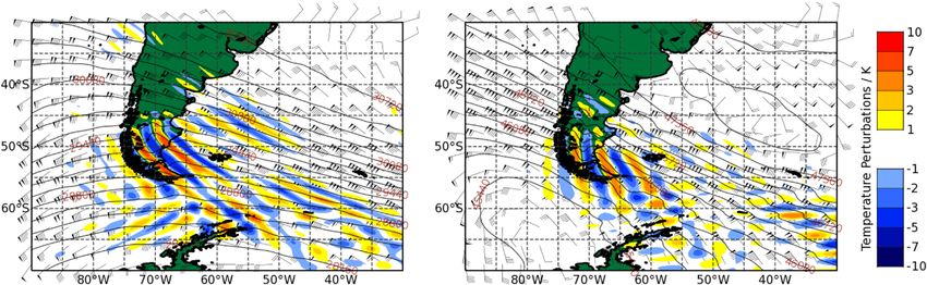
the mesospheric temperature background. In addition, GW momentum fluxes will be de-
duced following Ern et al. (2018).
Finally, a total of 59 radiosondes were released at Rio Grande (29 sondes) and El Calafate (30
sondes) during the September deployment of the HALO aircraft. At Rio Grande, a GRAW sound-
ing system with DFM-09 radiosondes (pressure determined by GPS) was used (GRAW 2019),
whereas at El Calafate a Vaisala sounding system with RS41 (some sondes with pressure
sensor) was employed (Vaisala 2020). The sondes yielded profiles of temperature, pressure,
humidity, and wind up to typical maximum altitudes of 25–30 km at a vertical resolution of
5–10 m depending on ascent rate. Table 2 summarizes all measurements available for the
characterization of GWs during SOUTHTRAC-GW.
Models. Flight planning for the HALO research flights was conducted with a lead time of
five to two days using the operational, deterministic forecasts of the Integrated Forecasting
System (IFS) of the European Centre for Medium-Range Weather Forecasts (ECMWF) and
the Met Office Unified Model. For the interpretation of the observational dataset we further
use ERA5 data. ERA5 is a global reanalysis dataset that is based on the IFS in cycle CY41R2
with 137 hybrid sigma/pressure (model) levels in the vertical, with the top level at 0.01 hPa.
This IFS cycle uses a sponge layer that starts at 10 hPa damping vertically propagating
GWs (Polichtchouk et al. 2017). Ehard et al. (2018) compared ground based lidar measure-
ments of GWs with corresponding IFS results and found that wave amplitudes are indeed
underestimated in the sponge layer. In addition, the sponge damps the zonal mean flow
though the small wavenumbers do not experience a very strong damping by the hyper-
diffusion type of damping (Polichtchouk et al. 2017). With respect to mesospheric tem-
peratures, the damping of GWs in the sponge layer weakens the upwelling (i.e., cooling)
in the summer hemisphere and the downwelling (i.e., warming) in the winter hemisphere
(Polichtchouk et al. 2017).
So far, ERA5 covers the period from 1979 to present. The high-resolution output is available
every hour and has a horizontal resolution of 31 km. For more details see Hersbach et al. (2020).
In some instances, we will show GW-induced temperature perturbations that are obtained as
T� = T639 − T106; i.e., we subtract ERA5 temperatures at the same spatial resolution but spec-
trally reduced to T106 from the full-resolution T639 fields.
Table 2. Airborne, ground-based, and satellite measurements suitable for characterization of GW during SOUTHTRAC-GW.
The variables u, υ, w, n, p, RH, T denote zonal, meridional, and vertical wind, number density, pressure, relative humidity,
and temperature. The terms du/dx and dυ/dx denote horizontal gradients of u and υ; Δz is vertical and Δx and Δy horizontal
resolution (in two dimensions).
Instrument Platform Measured quantity Height range Resolution Reference
ALIMA HALO n, T 20–90 km Δz = 1 km, 50 s This study
GLORIA HALO T, trace gases 5–15 km Δz = 200 m, Δx = 20 km Riese et al. (2014),
Δy = 20 km Friedl-Vallon et al. (2014)
BAHAMAS HALO u, υ, w, T, p In situ, 15 km 100 Hz Giez et al. (2017)
CORAL Rio Grande n, T 15–95 km 1 km, 1 h Kaifler and Kaifler (2020)
—— ——
SAAMER Rio Grande u, υ, uw , υw 80–100 km 3 km, hourly Fritts et al. (2010a)
MMARIA-SAAMER Multistatic u, υ, w, du/dx, dυ/dx 80–100 km 2 km, hourly Chau et al. (2017)
5-hole probe Stemme u, υ, w, T, p In situ 0–9 km 10 Hz Wildmann et al. (2021)
SABER Satellite Temperature 0–100 km Δz = 2 km, 3° along orbit Remsberg et al. (2008)
MetOp-A and MetOp-B Operational satellite T 20–40 km Δz = 1 km Rapp et al. (2018a)
Radiosondes Rio Grande u, υ, T, p, RH 0–30 km Δz = 5–10 m GRAW (2019)
Radiosondes El Calafate u, υ, T, p, RH 0–30 km Δz = 5–10 m Vaisala (2020)
AMERICAN METEOROLOGICAL SOCIETY
Unauthenticated 021 E877
A P R I L| 2Downloaded 09/23/21 03:30 AM UTC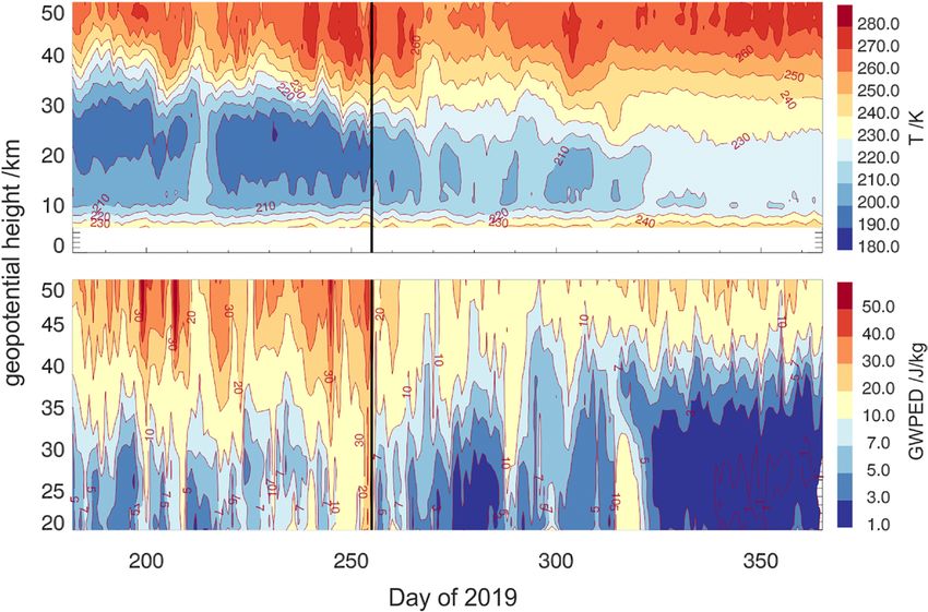
Flight planning of the glider flights in El Calafate was supported by the National Met Service
            of Argentina (Servicio Meteorológico Nacional) who provided dedicated forecasts with the
            Weather Research and Forecasting (WRF) Model.

            Atmospheric conditions during the campaign period
            The austral winter and spring season 2019 was unique in the sense that the southern polar
            vortex in late austral winter 2019 broke down early due to an SSW (Lin et al. 2020). According
            to classic metrics, it was a minor SSW, but it appeared as a major event as it changed the
            propagation conditions for MW markedly in September 2019. Already in August 2019, the
            vortex was offset slightly from the pole compared to the previous years and its shape became
            more elongated. The disturbance became striking in September 2019 when the vortex area
            shrunk and the center was displaced toward South America (cf. Fig. 8 in Dörnbrack et al. 2020).
               The remarkable weakening and warming of the polar vortex in the period from August to
            September is illustrated by the comparison of the zonal mean zonal wind and temperature in
            2019 with the 41 years long ERA5 climatology in Fig. 3. As depicted in Fig. 3, the zonal mean
            winds of the PNJ did not only decrease drastically but also its core was shifted poleward and
            downward compared to the climatology. Another striking feature is the strong negative wind
            anomaly near the equator at around 10 and 1 hPa extending to 15°–20°S. This anomaly is
            related to the easterly phase of the quasi-biennial oscillation (QBO; see also the MERRA-2
            analyses shown at https://acd-ext.gsfc.nasa.gov/Data_services/met/qbo). The magnitude of the
            warming amounts to about 30 K (see lower-right panel in Fig. 3 at latitudes south of 80°S).
               Associated with the warming in 2019, the zonal winds at ~1 hPa reversed suddenly at the
            beginning of September and remained negative or close to zero for the rest of the year. This

Fig. 3. (left) Zonal mean zonal winds (m s−1) for (a) August and (b) September 2019. Color shading is ERA5 data for the year
2019. Thick black lines are zonal mean winds (10 m s−1 increments) from the ERA5 climatological mean from 1979 to 2019.
The dashed black line is u = 0. (right) Color shading is ERA5 zonal mean temperature (K) for (c) August and (d) September
2019. Thick black lines are temperature anomalies (5-K increments) from the ERA5 climatological mean from 1979 to 2019.

            AMERICAN METEOROLOGICAL SOCIETY
                                                                                       Unauthenticated      021    E878
                                                                                               A P R I L| 2Downloaded 09/23/21 03:30 AM UTC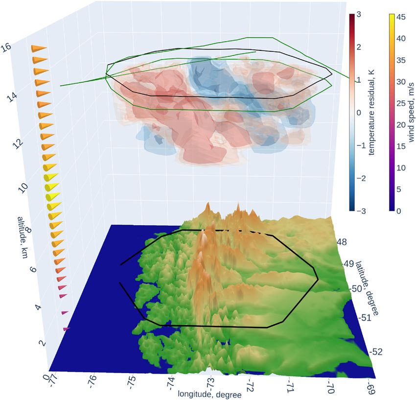
evolution generated a critical level for stationary MWs and confined their vertical propagation
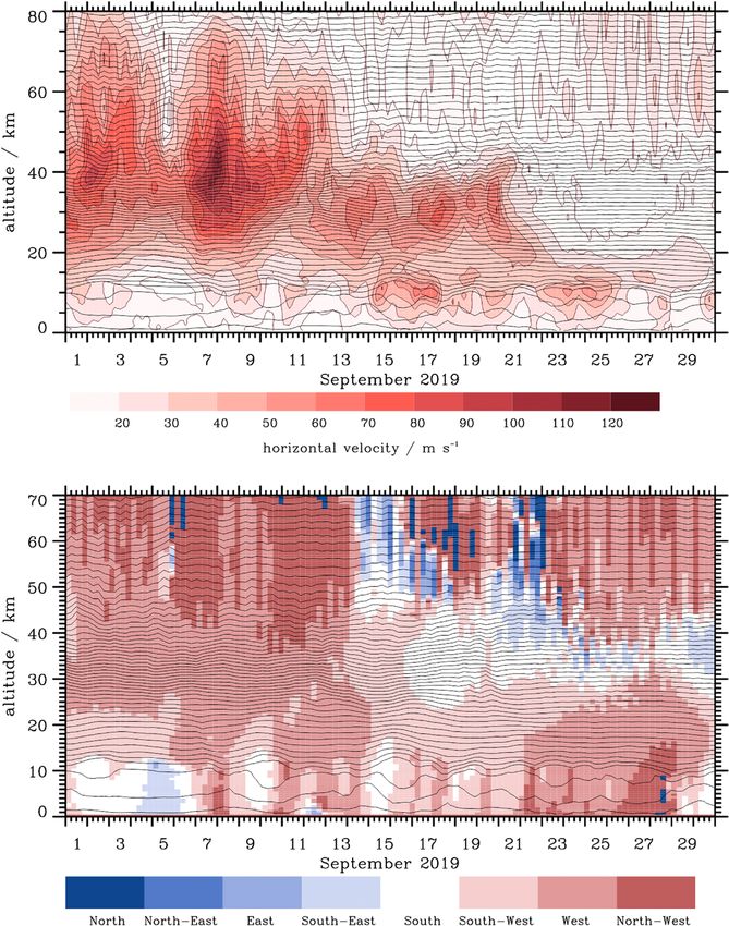
to altitudes below about 40 km from 13 September 2019 onward. This effect is clearly illus-
———
trated in Fig. 4 depicting the altitude–time sections of the horizontal wind (VHOR = √u2 + υ2 ,
where u and υ are zonal and meridional wind) and the wind direction calculated in a box
upstream of Patagonia (see also Fig. 8). Frequent weather systems approaching South America
produced a sequence of tropospheric jets near 10-km altitude and led to the quasi-continuous
low-level forcing of MWs. In the upper stratosphere, the PNJ weakened gradually during the
first half of September 2019, the wind reversed from westerlies to easterlies as indicated by
Fig. 4. Upstream profiles of ERA5 (top) horizontal wind VHOR and (bottom) wind direction for
September 2019. The data are averaged in the upstream box (80°W ± 5°, 50°S ± 5°).
AMERICAN METEOROLOGICAL SOCIETY
Unauthenticated 021 E879
A P R I L| 2Downloaded 09/23/21 03:30 AM UTC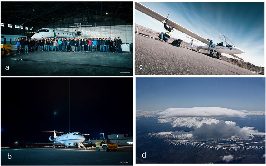
the 180° change of the wind direction. At the end of the month only the tropospheric jets and
           the tides remained as high wind patterns upstream of South America.
              To illustrate the spatial transitions of VHOR, of the geopotential height Z, and of the
           absolute temperature T associated with the stratospheric warming event, we show their
           respective anomalies VHOR*, Z*, and T* for August and September 2019 related to the
           41-yr ERA5 climatological mean at 100 hPa in Fig. 5. The warming and horizontal shift
           of the cold center of the polar vortex toward South America is clearly visible in the T*
           plots. The T* amplitude increased from August to September to values up to 25 K. Associ-
           ated with this T anomaly is the Z anomaly that switched from a weak planetary wave-2
           (PW2) pattern in August to a strong PW1 pattern in September (see also Shen et al. 2020).
           In September, related to the weakening and shrinking of the polar vortex, VHOR over
           Patagonia decreased south of 50°S and increased north of about 50°S leading to weaker
           than normal winds toward Antarctica.
              Notably, the effect of the SSW can also be clearly seen in middle atmosphere temperature
           and wind measurements acquired at EARG as well as in MetOp RO measurements in the re-
           gion (Figs. 6 and 7). Figure 6 shows daily mean (i.e., tidal components removed) zonal wind
           measurements from SAAMER for the period 1 July–31 December 2019. The mesospheric
           observations show mainly westerly winds with maximum values of about 50 m s−1 until 12
           September after which the winds at all observed altitudes changed to easterly direction with
           maximum values of about 20 m s−1 until the end of October. Hence, the mesospheric circulation

Fig. 5. Color shading shows anomalies of the (a),(b) horizontal wind, (c),(d) geopotential height, and (e),(f) temperature
at 100 hPa with respect to the 41-yr ERA5 climatological mean for (top) August and (bottom) September 2019. The black
lines in the left column show the mean wind. Note, the temperature scale is different for August and September.

           AMERICAN METEOROLOGICAL SOCIETY
                                                                                     Unauthenticated      021    E880
                                                                                             A P R I L| 2Downloaded 09/23/21 03:30 AM UTC
changed to a summer-like
state as early as in the mid-
dle of September. In the cli-
matological mean the tran-
sition would be expected
to occur about one month
later (de Wit et al. 2017).
This early transition to a
summer-like state is well
known from correspond-
ing mesospheric wind ob-
servations in the Northern
Hemisphere as being due to
the changed GW propaga-
tion characteristics during
SSW (Hoffmann et al. 2002).
Interestingly, the wind struc-
ture in the period from 12
September until the end of
October also deviates from
a typical summer circulation
since easterly winds are ob-
served in the entire SAAMER
observation volume whereas
in the climatological mean
easterly winds are only ex- Fig. 6. (top) Zonal wind measurements during July–December 2019 with
SAAMER. (bottom) Composite of lidar measurements with the ground based
pected below ~90 km, with
system CORAL and ALIMA. From the beginning of August to the beginning
westerly winds usually oc- of October the laser of the CORAL system failed such that no ground based
curring above. Hence, the measurements are available during this time. The gap is partly filled with
unusual filtering conditions SABER data and with data from the ALIMA system from HALO flight legs in
for GW in the stratosphere the vicinity of Rio Grande. In both panels, the black vertical line marks the
coincided with a very unusu- time of HALO flight ST08.
al mesospheric circulation
in the entire altitude range from 80 to 100 km as probed by SAAMER. Only after the begin-
ning of November, a typical summer circulation is observed (cf. to Fig. 3 in de Wit et al. 2017).
The composite of CORAL, SABER and ALIMA temperature measurements in the upper
stratosphere and mesosphere also reveals characteristic signatures as expected for an SSW
(lower panel of Fig. 6). Already in the end of August, the stratopause moves up, which is
in agreement with several previous observations and modeling studies of SSW effects on
the mesosphere (e.g., Siskind et al. 2010; Limpasuvan et al. 2016). After the beginning of
November, CORAL measured a cold summer mesopause with temperatures falling as low as
150 K above ~80-km altitude, which is consistent with the SAAMER observations of a sum-
mer circulation after the same date.
To get a first impression of the temporal evolution of stratospheric GW activity in the region we
next turn to the MetOp RO measurements of temperatures and GWPED in Fig. 7. Here, we clearly
see signatures of the SSW in both parameters in the stratosphere. The shown RO measurements
are daily averages over a box range from 55° to 64°S and from 70° to 0°W, which is the region of
the Drake Passage and eastward along the Southern Ocean centered at 60°S. This averaging has
been chosen due to the scarce sampling of the MetOp satellites at these latitudes [see Fig. 1a in
Rapp et al. (2018b) for typical daily sampling statistics of MetOp RO measurements]. Figure 7 clearly
AMERICAN METEOROLOGICAL SOCIETY
Unauthenticated 021 E881
A P R I L| 2Downloaded 09/23/21 03:30 AM UTCFig. 7. (top) Stratospheric temperatures (as mean for 55°–64°S and 70°–0°W) obtained from radio
occultations on board the MetOp-A and MetOp-B satellites (Rapp et al. 2018a). (bottom) Corre-
sponding GW potential energy densities, also from MetOp-A and MetOp-B. In both panels, the
black vertical line marks the time of HALO flight ST08.
shows a sudden and notable increase of stratospheric temperatures after 12 September (marked
with the black vertical line). Even more interesting, right after this date the observed GWPEDs
decrease rapidly above ~40 km as a consequence of the critical level for MWs seen in Fig. 4.
In summary, the SOUTHTRAC-GW mission took place during the evolution of a rare South-
ern Hemisphere minor SSW, which had pronounced effects on the propagation characteristics
of GW and thus also on the background state of the middle atmosphere.
Mission overview and early results
SOUTHTRAC-GW commenced on 9 September 2020 with the transfer flight from Buenos Aires
to Rio Grande followed by six research flights until 26 September. The six local research flights
started from and returned to the naval air base at Rio Grande airport and were conducted in
darkness to guarantee optimal operation conditions for ALIMA. During all flights, success-
ful measurements with the airborne instruments as listed in Table 2 were obtained. Partly,
the ALIMA measurements were deteriorated due to icing on its optical window in the aircraft
fuselage. This led to signal degradation and hence a limited altitude coverage during two of
the flights (ST07, ST10). Overall, the data quality of ALIMA and all other GW instruments
was above expectations to achieve the scientific goals of the mission.
The flight tracks of all seven GW-related research flights are shown in Fig. 8. The general
strategy for the planning of these flights was to both observe excitation regions, e.g., over
the Andes or over the Antarctic peninsula (see corresponding cross mountain legs), and then
to follow the waves into and along the polar vortex. Hence, many flight legs are long and
straight at a constant pressure altitude to allow for optimal sampling of GW characteristics.
Hexagon-shaped flight tracks were designed for tomographic characterization of tropospheric
GW close to their source with GLORIA (i.e., flight tracks of ST12 and ST14). The location of
the cross mountain legs as shown in Fig. 8 reflects the fact that during most of the research
AMERICAN METEOROLOGICAL SOCIETY
Unauthenticated 021 E882
A P R I L| 2Downloaded 09/23/21 03:30 AM UTCflights MW forcing occurred
to the north of Rio Grande.
Vertical profiles of hori-
zontal velocity and wind
direction measured by the
radiosondes at Rio Grande
are shown in Fig. 9. A ninth-
order polynomial was fitted
to the data of the ascending
sondes in order to reveal the
background wind conditions
and to fill gaps in the data
caused by poor signal recep-
tion. Surface winds at Rio
Grande were mainly around
10–15 m s−1 (Fig. 9a) with
varying westerly to south-
erly wind direction (Fig. 9b).
Wind direction in the low and
midstratosphere was also
mainly westerly to south-
westerly and wind speed
significantly decreased from
around 40–60 m s−1 to al- Fig. 8. Map showing the flight tracks of the seven GW flights of HALO dur-
most zero at 30-km altitude ing the SOUTHTRAC-GW mission. The typical flight distance of each flight
is ~7,000 km. The gray box in the west of the tip of South America is the
after 20 September. These
domain over which upstream wind profiles have been calculated (Fig. 4).
findings for the stratospheric
winds are in agreement with
the ERA5 data for the upstream region presented in Fig. 4. Fluctuations in the stratospheric
horizontal wind data caused by GWs with an apparent vertical wavelength smaller than
10 km were most pronounced on 25 and 26 September, i.e., during flight ST14. Peaks in
the wavelet power spectra of these profiles are found at an apparent vertical wavelength of
around 5 km (not shown).
Table 3 provides a list of all GW flights, their date, length, research objectives, and sum-
marizes the specific phenomena observed during the flights.
Figure 10 gives an overview of the vertical energy fluxes derived from the BAHAMAS in
situ measurements at flight level for all straight flight legs of the GW flights (with a maximum
length of 2,300 km at flight levels between 10 and 14 km). For the analysis the legs were di-
vided into sublegs with typical lengths of ~300 km and then analyzed following the procedure
described in Bramberger et al. (2017) which also provides a discussion of important assump-
tions and restrictions of such an analysis. Except for one leg all energy fluxes are positive
indicating predominant upward GW propagation. The fluxes vary between 0 and 25 W m−2,
which is similar to the range of MW-induced energy fluxes reported by Smith et al. (2016)
from measurements during DEEPWAVE.
As an example for the very different atmospheric conditions before and after the SSW we
contrast ALIMA observations from flights ST08 and ST12. In Figs. 11 and 12, the altitude
versus time diagrams of both observed temperatures and temperature perturbations clearly
show that GW were able to propagate deeply into the mesosphere during ST08 but reached a
critical level already at 40 km during ST12 as expected from our analysis of horizontal winds
in Fig. 4. ST12 was the flight with strongest vertical energy fluxes at flight level (see Fig. 10).
AMERICAN METEOROLOGICAL SOCIETY
Unauthenticated 021 E883
A P R I L| 2Downloaded 09/23/21 03:30 AM UTCFig. 9. Vertical profiles of (a) horizontal wind and (b) wind direction measured by the radiosondes
at Rio Grande. Raw data of the ascending (descending) sondes are given in dark gray (light gray)
with ninth-order polynomials fitted to the ascending data in black. The horizontal shift of the
individual profiles is 9 m s−1 (63°) per 3-h time difference for velocity (direction) whereupon days
without soundings are omitted. Vertical dotted lines mark the zero reference of the individual
profiles, and the distance between ticks is 10 m s−1 (90°) for velocity (direction). Date and time of
the first sounding are given on each day.
The observations during ST08 show several interesting features: during the cross-mountain
legs of ST08 (legs 1–2 and 2–3), distinct GW phases were observed by ALIMA with very large
amplitudes in excess of 10 K (maximum values are 25 K; not shown). A prominent change
in vertical wavelength is observed around 40 km and again at 55-km altitude, with signifi-
cantly steeper phase lines between 40 and 55 km. Preliminary analysis involving a spectral
decomposition of the observations and the spatiotemporal development of the situation seen
in ERA5 data suggests that this could be explained by the superposition of multiple wave
modes that interact with the background wind and hence change their vertical wavelength
Table 3. SOUTHTRAC-GW flights.
Flight Date Start (UTC) Length Objectives (see Table 1) Summary
ST07 9 Sep 2019 0700 6 h 30 min 2,3 MW, deep propagation
ST08 11/12 Sep 2019 2300 8 h 31 min 1, 2, 3, 4, 5 MW, deep propagation, breaking, secondary GWs, refraction into
the PNJ and along the GW belt
ST09 13/14 Sep 2019 2300 9 h 6 min 2, 3, 5 NOGWs upstream Andes, MW
ST10 16/17 Sep 2019 2300 8 h 58 min 2, 3, 4, 5 MWs and nonorographic GW in vicinity of tropospheric jet
streams, wave breaking, and effects on trace gas distributions
ST11 18/19 Sep 2019 2300 8 h 13 min 2, 3, 5 MW propagation from 40°S to jet exit region at 60°S; PNJ edge
disturbed by GWs
ST12 20/21 Sep 2019 2300 9 h 10 min 1, 2, 3, 4, 5 MW, time variation at source, refraction into the PNJ, upwind
propagation, secondary GW, 3D tomography
ST14 25/26 Sep 2019 2330 9 h 17 min 1, 2, 3, 5 MW over the southern Andes and Antarctic Peninsula with weak
forcing, horizontal propagation into Drake Passage, 3D tomography
AMERICAN METEOROLOGICAL SOCIETY
Unauthenticated 021 E884
A P R I L| 2Downloaded 09/23/21 03:30 AM UTC(not shown). At approximately 65 km, the
ALIMA measurements suggest unstable
breakdown of the GW and secondary wave
generation: i.e., wave amplitudes of the
primary GW decrease strongly above this
altitude while simultaneously occurring op-
positely aligned smaller-scale phase fronts
could be interpreted as features of secondary
waves as discussed in N. Kaifler et al. (2017).
The details of this vertical structure and the
Fig. 10. Energy fluxes measured with the nose-tip probe of
mentioned signatures for wave breaking and
HALO on straight and leveled flight legs vs flight number.
secondary GWs will be presented in detail
in a future paper.
Further into the flight, clear GW signatures are also observed along the polar vortex at 1 hPa
(leg 3–4, see also lower-left panel in Fig. 11) and in the Drake Passage (legs 4–5 and 5–6).
Based on these observation and taking into account preliminary time-dependent numerical
Fig. 11. (top) Contour plots of temperatures derived from ALIMA observations vs altitude and time for research flight (a)
ST08 and (c) ST12; see Table 3. Vertical lines and numbers mark the start and endpoints of the flight legs. (b),(d) Corresponding
flight tracks with numbers indicating the start and endpoint of flight legs with horizontal wind speeds at 1 hPa shown
as colored contours in the background. Gray contour lines show isolines of geopotential height (m).
AMERICAN METEOROLOGICAL SOCIETY
Unauthenticated 021 E885
A P R I L| 2Downloaded 09/23/21 03:30 AM UTCFig. 12. (a),(c) IFS temperature perturbations compared to (b),(d) ALIMA temperature perturbations along the flight tracks
of flights (left) ST08 and (right) ST12.
modeling of the situation as well as ray tracing, we hypothesize that the observed GW were
excited by flow over the Andes. Subsequently, they were refracted into the PNJ and then
propagated eastward in the Drake Passage toward 60°S. These high-resolution observations
in time and space (in combination with yet to be completed numerical simulations) may hence
provide compelling evidence that the refraction of MWs does occur in nature and is one of
the sources for the GW belt as suggested by GW-resolving modeling (Sato et al. 2012), inter-
pretation of ground based observations during DEEPWAVE (Ehard et al. 2017), and satellite
observations (Hindley et al. 2019). We will test this hypothesis incorporating high-resolution
three-dimensional modeling of this particular case with the Eulerian/semi-Lagrangian fluid
solver (EULAG) in a future paper (see, e.g., Wilms et al. 2020, and references therein).
Figure 12 juxtaposes the ALIMA measurements during ST08 and ST12 with 1-hourly
operational IFS analyses and short-term forecasts. The larger-scale features in the observa-
tions are amazingly well resolved by the IFS. Minor differences are observed with regard to
exact timing, vertical extent and amplitudes of the GWs as well as smaller-scale features.
Again, these are issues that will be further investigated applying high-resolution numerical
modeling.
Since the IFS reproduces the gross features of the GW signatures during ST08 fairly well we
may further use the model to investigate whether the model shows signatures of GW refraction
AMERICAN METEOROLOGICAL SOCIETY
Unauthenticated 021 E886
A P R I L| 2Downloaded 09/23/21 03:30 AM UTCFig. 13. ERA5 temperature perturbations T� = T639 − T106 (K; color shaded in red and blue colors), geopotential height (m;
solid lines), and horizontal wind (half barb = 2.5 m s−1, full barb = 5 m s−1, and pennant = 25 m s−1) as function of latitude
and longitude in the region of the southern Andes and Antarctic Peninsula during research flight ST08. ERA5 fields are
shown for 0000 UTC, i.e., 1 h into the flight. Shown are (left) 10 hPa and (right) 1 hPa.
and downwind advection into the GW belt. As shown in Fig. 13, this is indeed the case: this
figure shows 2D cross sections of IFS temperature perturbations, geopotential height, and
horizontal winds in the region of the southern Andes and the Antarctic Peninsula at 10 and
1 hPa. At 10 hPa, those GWs
that were excited both by
the flow over the Andes and
the Antarctic Peninsula are
advected downwind and
poleward. The phase fronts
at 10 hPa are oriented nearly
perpendicular to the west-
erly stratospheric wind di-
rectly above the mountains.
They tilt poleward over the
Drake Passage in response
to the gradient of the zonal
wind. At 1 hPa the wind
has turned to northwest-
erlies and also the phase
fronts have rotated into the
wind, hence providing evi-
dence for wave refraction.
However, due to the weaker
winds in the polar vortex,
the GW cannot propagate as
far poleward as at lower lev-
els. Hence, the good agree-
ment between observations
and IFS model and the clear Fig. 14. A 3D tomographic retrieval of GWs observed with GLORIA during
flight ST12 on 19 Sep 2019 is shown by means of isosurfaces. Thin lines
signature for MW propaga-
show the flight path: black—the hexagonal flight path used for the de-
tion into the GW belt make picted 3D retrieval; green—the remainder of the flight. The thick black line
a strong case for refraction is the ground track of the hexagonal flight pattern. The cones show the IFS
and downwind advection upstream wind profile.
AMERICAN METEOROLOGICAL SOCIETY
Unauthenticated 021 E887
A P R I L| 2Downloaded 09/23/21 03:30 AM UTCcontributing to the formation of the GW belt in support of earlier studies (Sato et al. 2012;
Ehard et al. 2017; Hindley et al. 2019).
As a further initial highlight of our observations, we turn to the tomographic analysis of
GLORIA measurements from the second hexagon of flight ST12. On 20 September, strong
southwesterly winds in the lower troposphere (>10 m s−1) generated a MW over the Andes
(Fig. 14). The maximum amplitude was forecasted in the area about one flight hour from Rio
Grande, providing an opportunity to spend several hours in the target region and, in particular,
to encircle the investigated air volume twice by a hexagonal flight pattern with a diameter
of ~350 km. Below flight level the 3D temperature structure was inferred from the infrared
emissions measured by GLORIA by applying a tomographic retrieval (Ungermann et al. 2011;
Krisch et al. 2017). The largest MW amplitudes were seen directly above the Andes in the west-
ern half of the hexagon. As expected for MWs, their phase fronts were oriented under a slight
angle with respect to the mountain ridge and tilted southwestward, against the wind. Given
the measurement setup, this GW event provides an excellent case for studying the excitation
and propagation of the waves in the upper troposphere/lower stratosphere. Propagation to
higher altitudes and dissipation at 40-km altitude (as suggested by the strongly decreased
amplitudes above this altitude) was observed by ALIMA (Fig. 11). Thus, the combination of
the two remote sensing instruments can be used to characterize the GW dynamics over almost
the entire depth of the atmosphere.
Finally, we also present an example of a Stemme glider flight to illustrate the type
of data and scientific potential of these measurements (Fig. 15). An overview of these
Fig. 15. (a) Flight track of the Stemme glider on 14 Sep 2019. Map data © OpenStreetMap-Contributors, SRTM; map:
© OpenTopoMap (CC-BY-SA). (right) Corresponding time series of (b) flight altitude, (c) vertical wind, and (d) turbulent
kinetic energy measured along the flight track.
AMERICAN METEOROLOGICAL SOCIETY
Unauthenticated 021 E888
A P R I L| 2Downloaded 09/23/21 03:30 AM UTCmeasurements is presented in Wildmann et al. (2021). Figure 15a presents the flight track of
one long-distance soaring flight from El Calafate and back as flown on 14 September 2019.
Figure 15b shows the corresponding altitude profile. In search for the strongest updrafts the
Stemme climbed several times in the ascending branches of mountain lee waves. Hence,
the observations were not conducted at a fixed altitude like during HALO flights but are
taken along a sawtooth pattern. Correspondingly, the scientific interpretation of these data
will need to take the motion of this measurement platform into account. An example for
such measurements is the vertical wind and turbulence kinetic energy data (derived from
high-resolution wind measurements with the 5-hole probe mounted under the wings of the
glider; see Wildmann et al. 2021), which are also shown in Figs. 15c and 15d, respectively. It
shows that in periods of soaring in the updraft of the waves, high vertical velocity (up to 8 m s−1)
and low turbulence prevails, whereas higher turbulence is detected in phases of the flight when
the glider was outside the updraft branch of the waves (low vertical velocity and descending
altitude). Despite the complication of changing flight altitudes, this dataset will be used to
investigate tropospheric lee waves and to evaluate numerical weather prediction models.
For a single case study, Wildmann et al. (2021) show that these measurements compare
well to the predictions of a mesoscale model at 1-km horizontal resolution, but differences
remain between modeled and observed magnitude of vertical velocities and the locations
of the waves.
Summary and outlook
SOUTHTRAC-GW was the first airborne field campaign targeting GW dynamics in the at-
mosphere from the troposphere up to the mesopause region at the world’s strongest strato-
spheric GW hotspot, i.e., the region of the southern Andes and the Antarctic Peninsula.
One transfer flight from Buenos Aires and six research flights from Rio Grande, Argentina,
were conducted with the German research aircraft HALO in September 2019 each cover-
ing a distance of about 7,000 km. The total number of flight hours was 59.75. During these
flights a comprehensive instrument package of remote and in situ instruments allowed us
to characterize GWs from 5- to 80-km altitude. The campaign period coincided with the
occurrence of a rare SSW which created a critical level for stationary MWs at about 40-km
altitude after 13 September with pronounced effects on subsequent GW propagation and
corresponding mesospheric temperatures and winds. Two of the research flights were con-
ducted before and five after the occurrence of the stationary wave critical level at 40 km.
Hence, SOUTHTRAC-GW succeeded to take measurements both during conditions of deep
GW propagation into the upper mesosphere and during conditions where GWs encountered
wave breaking and dissipation already at or below 40-km altitude. Thus, the September
2019 period may be considered as a condensed period of the transition from a winter to a
summer regime and allowed us to take observations during both atmospheric states within
a short period of time.
Preliminary analysis of our measurements and accompanying model results reveal strong
evidence for MW excitation over the Andes and subsequent vertical as well as horizontal
propagation including refraction and downwind advection into the PNJ and along the GW
belt. Our findings strongly suggest that these processes are one of the reasons for the early
development of the GW belt in the vicinity of the southern Andes and Antarctic Peninsula.
More detailed numerical modeling and data analysis (including ray tracing) will be conducted
in the coming months to corroborate these preliminary observational results. In addition,
during two of our research flights we were able to comprehensively characterize the full 3D
structure of upper tropospheric GWs excited over the Andes. Further analysis will yield un-
precedented details of the properties of such waves. The remote sensing measurements by
ALIMA and GLORIA will hence be a benchmark dataset for future high-resolution modeling.
AMERICAN METEOROLOGICAL SOCIETY
Unauthenticated 021 E889
A P R I L| 2Downloaded 09/23/21 03:30 AM UTCAlso a clear-cut case with MW excitation over the Antarctic peninsula was characterized by
airborne measurements. Furthermore, several of the research flights reveal indications of
GW breaking and secondary wave excitation as indicated by corresponding scales and spa-
tiotemporal morphologies of observed phase fronts (N. Kaifler et al. 2017). Secondary wave
excitation is an exciting topic (Becker and Vadas 2018) which remains very difficult to probe
and for which numerical simulations require enormous efforts (e.g., Dong et al. 2020). Hence,
these data have the potential to serve as an invaluable guidance for high-resolution modeling
of such processes and will allow us to yield a deeper understanding of the corresponding
fundamental dynamics of GWs.
In the coming months, the preliminary results mentioned above will be further scruti-
nized including dedicated efforts of high-resolution modeling, and including additional data
sources like from satellite instruments like AIRS (e.g., Hindley et al. 2019). In addition, we
will consider in how far the results obtained from combined observations and modeling will
be useful for the important challenge of formulating improved gravity wave parameteriza-
tions for climate models (Plougonven et al. 2020). Furthermore, improvements of the ALIMA
instrument to incorporate an iron resonance lidar channel (B. Kaifler et al. 2017) are under
way which will extend the measurement range of ALIMA to 110 km and also add the abil-
ity to measure vertical winds. With these instrumental improvements, a follow-up airborne
mission is currently being planned for Northern Hemisphere winter 2021 during which the
same set of instruments on HALO will be utilized to further characterize the role of the polar
vortex for GW propagation and its impact on the middle atmosphere circulation.
Acknowledgments. The authors gratefully acknowledge the enormous hospitality of the Argentinian
Navy who hosted HALO and our team in their facilities at the Naval air base of Rio Grande. We also
thank the Argentinian and Chilean authorities for their permission to perform research flights in
their airspace. Thanks also for excellent support by the DLR facility for Flight Experiments (FX) and
Klaus Ohlmann, the ingenious pilot of the Stemme glider. We are grateful for Annelize van Niekerk
(UK MetOffice) for providing the Unified Model simulations applied during flight planning of HALO
flights. The National Meteorological Service of Argentina (SMN) and the German Weather Service
(DWD) supported the SOUTHTRAC-GW campaign by providing regional forecasts. Alejandro Godoy,
Nicolas Rivaben (SMN) and Tobias Göcke (DWD) participated in the forecast team. Collaboration with
AvN was established in the framework of the ISSI Team “New Quantitative Constraints on OGW Stress
and Drag” at the ISSI Bern. This work was partly funded by the Federal Ministry for Education and
Research under Grants 01LG1907 (project WASCLIM) in the frame of the Role of the Middle Atmo-
sphere in Climate (ROMIC) program as well as by internal funds of the German Aerospace Center, the
Karlsruhe Institute of Technology, and Forschungszentrum Jülich. The university groups involved
were funded by the German Science Foundation (DFG) through the HALO-SPP. Further support by the
German Science foundation under Grants GW-TP/DO1020/9-1 and PACOG/RA1400/6-1 in the frame
of the DFG research group MS-GWAVES (FOR1898) is also acknowledged. Access to ECMWF data was
granted through the special project “Deep Vertical Propagation of Internal Gravity Waves.”
Data availability statement. Airborne, CORAL, and radiosonde data can be accessed via the HALO
database under https://halo-db.pa.op.dlr.de. According to HALO data policy, data are freely available
from 30 months after the end of the mission, i.e., from June 2022. Before this date, data shown in
this publication are available from the first author upon request. IFS forecast and ERA5-data data
can be found under www.ecmwf.int/en/forecasts/datasets/set-i and www.ecmwf.int/en/forecasts/datasets
/reanalysis-datasets/era5, respectively. MetOp RO data are available from www.romsaf.org. SAAMER data
can be downloaded from the Madrigal database under http://millstonehill.haystack.mit.edu. SABER data
are available at http://saber.gats-inc.com.
AMERICAN METEOROLOGICAL SOCIETY
Unauthenticated 021 E890
A P R I L| 2Downloaded 09/23/21 03:30 AM UTCYou can also read