Dynamic Systems Approach in Sensorimotor Synchronization: Adaptation to Tempo Step-Change - Frontiers
←
→
Page content transcription
If your browser does not render page correctly, please read the page content below
ORIGINAL RESEARCH
                                                                                                                                              published: 21 June 2021
                                                                                                                                     doi: 10.3389/fphys.2021.667859

                                                Dynamic Systems Approach in
                                                Sensorimotor Synchronization:
                                                Adaptation to Tempo Step-Change
                                                Nima Darabi and U. Peter Svensson*
                                                Department of Electronic Systems, Norwegian University of Science and Technology, Trondheim, Norway

                                                This paper presents a dynamic systems model of a sensorimotor synchronization
                                                (SMS) task. An SMS task typically gives temporally discrete human responses to some
                                                temporally discrete stimuli. Here, a dynamic systems modeling approach is applied
                                                after converting the discrete events to regularly sampled time signals. To collect data
                                                for model parameter fitting, a previously published pilot study was expanded. Three
                                                human participants took part in an experiment: to tap a finger on a keyboard, following a
                                                metronome which changed tempo in steps. System identification was used to estimate
                                                the transfer function that represented the relationship between the stimulus and the
                                                step response signals, assuming a separate linear, time-invariant system for each tempo
                                                step. Different versions of model complexity were investigated. As a minimum, a second-
                           Edited by:           order linear system with delay, two poles, and one zero was needed to model the most
                      Franca Tecchio,
    Consiglio Nazionale delle Ricerche          important features of the tempo step response by humans, while an additional third pole
                           (CNR), Italy         could give a somewhat better fit to the response data. The modeling results revealed
                        Reviewed by:            the behavior of the system in two distinct regimes: tempo steps below and above the
                      John G. Holden,
University of Cincinnati, United States
                                                conscious awareness of tempo change, i.e., around 12% of the base tempo. For the
                     Elka Korutcheva,           tempo steps above this value, model parameters were derived as linear functions of
       National University of Distance          step size for the group of three participants. The results were interpreted in the light of
             Education (UNED), Spain
                                                known facts from other fields like SMS, psychoacoustics and behavioral neuroscience.
                  *Correspondence:
                    U. Peter Svensson           Keywords: sensorimotor synchronization, period correction, rhythmic perception, system identification, root
              peter.svensson@ntnu.no            locus analysis, pole/zero systems, frequency domain, tempo step-change

                   Specialty section:
         This article was submitted to          INTRODUCTION
                     Fractal Physiology,
               a section of the journal         Sensorimotor synchronization (SMS) is defined as the coordination of rhythmic movement (motor)
               Frontiers in Physiology
                                                with an external rhythm (sensory) (Repp, 2005; Repp and Su, 2013). Such rhythmic coordination
        Received: 19 February 2021              of perception and action, or the rhythmic synchronization between a timed sensory stimulus and
           Accepted: 05 May 2021
                                                a motor response (Michon and Van der Valk, 1967), is often studied in the context of rhythmic
          Published: 21 June 2021
                                                perception and collaboration, especially music performance.
                             Citation:             One standard experiment in the study of SMS deals with the task of synchronizing an action
          Darabi N and Svensson UP
                                                to a temporally regular (isochronous) series of impulses and has applications beyond music co-
(2021) Dynamic Systems Approach in
       Sensorimotor Synchronization:
                                                performance, such as in dance (Miura et al., 2011) or computer gaming (Bégel et al., 2017).
  Adaptation to Tempo Step-Change.              When reducing the input (the sensory stimulus) to a metronome, i.e., an isochronous sequence
           Front. Physiol. 12:667859.           of tones or clicks, the action is often reduced to a simple task of hand clapping or finger tapping
    doi: 10.3389/fphys.2021.667859              in synchronization with the input (Repp, 2005). A variety of models have been used to study the

Frontiers in Physiology | www.frontiersin.org                                        1                                         June 2021 | Volume 12 | Article 667859
Darabi and Svensson                                                                                    Tempo Step Response in Frequency-Domain

relationship between such input and output. These models                  processes called phase and period error correction processes that
typically rely on a simple assumption that, based on observations         will be briefly reviewed in section “Event and Interval Variables
of previous beat timings, the participant can predict the timing of       and the Choice Between the Period Error Correction and Phase
the next beat and make anticipatory actions, for example aiming           Correction Process” due to their relevance to the stages of data
at being synchronous to it. In this paper, we are bringing models         preparation in this work. He also made a distinction between
from dynamical systems theory and control systems engineering             internal processes and external timing and attempted to explain
to the study of SMS and applying them on data from a task                 the often observed overshoot for step responses and showed
of synchronization to a suddenly changing metronome tempo.                that period correction is slower for undetected than for detected
The primary goal is to apply dynamic systems modeling to the              changes, even when they were of the same magnitude (Repp,
inherently discrete-time system of an SMS task. The use of a              2001a,b), implying that phase correction is rapid and automatic,
separate linear, time-invariant system for each tempo step is a           whereas period correction can be dependent on awareness of a
limitation, but model parameter trends might be developed into            tempo change (Repp, 2001a,b) (Hary and Moore, 1985) reported
more advanced non-linear models, which could be applied to                adaptation to subliminal step changes to be very slow and
more general stimulus signals.                                            gradual. Thaut M. H. et al. (1998) investigated the adaptation by
                                                                          five subjects to an unexpected step change of 2, 4, or 10%, for
History                                                                   an input interval of 500 ms in a finger-tapping task and reported
Studies on rhythm and perception started in the early years of            a strategy shift based on the percentage of the introduced step
experimental psychology with pioneer works by Stevens (1886)              change. They also reported a relatively rapid adaptation to both
and Wilhelm Wundt back in the 1890s [cited in Blumenthal                  large and small step changes, though the overshoot occurred
(1975)]. Early work included experimental studies on the speed            only after large, detectable changes. Repp and Keller (2004)
of synchronization with an external rhythm (Nicholson, 1925)              observed the suppression of period correction, but not phase
[cited in Delignières et al. (2004)] and properties of asynchrony         correction, when asking participants to continue tapping at the
in adaptation to different tempos, which led to the definition of         initial tempo and ignoring the step change. They concluded
upper limits of the human rates (Woodrow, 1932). Later, notable           that phase correction is a lower-level cognitive process, whereas
contributions were made in the 1950s and 1960s through the                period correction could have higher-level cognitive components.
works of Paul Fraisse [cited in Repp (2005)] and Michon and               Repp (2002) also considered phase correction to be purely
Van der Valk (1967). Michon studied the response to rhythmic              specific to SMS tasks whereas period correction could be more
perturbations including step changes, ramps and sinusoidals and           related to expressing timing in music. It is reported that over-
sums of sinusoidals. He also made the first attempt at formulating        correction above the threshold of awareness happens as a result
a standard set of descriptive terms to describe research on SMS.          of participants adjusting the timing of their taps by a larger
In later years Bruno H. Repp (Repp and Keller, 2004; Repp, 2010)          amount than would be necessary to compensate for the full
and Jeff Pressing (Pressing and Jolley-Rogers, 1997; Pressing,            asynchrony (Van Der Steen and Keller, 2013). The observation
1998, 1999) presented several important findings, including two           of overshoot has also been reported for continuous, rather than
extensive overview studies (Repp, 2005; Repp and Su, 2013).               sudden, step-changes. Schulze observed a systematic alternation
                                                                          of under-adjustment and over-adjustment of period and phase
Study of Sudden Step Changes                                              correction in synchronization with a metronome that smoothly
One particular task, which is common in the studies of SMS, is            changed tempo, from slow to fast (accelerando) or from fast to
to respond to sudden tempo changes. Michon used inter-onset               slow (ritardando) (Schulze and Vorberg, 2002). For experiments
intervals (IOIs) (the time between two consecutive clicks) of 600,        combining step changes with phase see Large et al. (2002), and
1200, and 2400 ms and step changes of 8, 16, and 32% of the base          with antiphase tapping, see Thaut and Kenyon (2003).
value, and one step up and one step down for each test on five               Fraisse and Repp (2012) reported a situation in which
subjects (Michon and Van der Valk, 1967). The results revealed            participants began to synchronize with a sequence when its
an initial overshoot in the rate of the response for increasing           tempo was not known in advance and observed that about three
tempo changes, as well as an undershoot for decreasing ones,              taps were needed to tune in to a sequence if the tapping started
generally within 4–5 taps. He proposed a linear predictor model           immediately after the first tone. From the third stimulus (or the
that could account for 70% of the data collected from three of            third cycle in the case of a simple repeated rhythm) onward,
his five subjects. Parameterizing the experiment and identifying          simultaneity was achieved with an error of less than 50 ms.
the parameters he spotted some non-linearity; that the quality
of performance depended on the step size and the baseline IOI.
However, he did not elaborate on the nature of this dependency            Discrete and Continuous Approaches to
nor included a higher resolution of tempo changes or a variety of         SMS
tempo baselines.                                                          In studies of SMS, there are two main theoretical approaches:
   Later studies started to make a difference between the                 information processing and dynamic systems theory (Torre
subliminal step changes that are below the threshold for                  and Balasubramaniam, 2009). Information-processing theory
conscious perception, and the supraliminal changes that are               describes the rhythmic responses and stimuli as event-based
above that threshold (Thaut M. et al., 1998; Thaut and Kenyon,            discrete time series and aims at describing hypothetical internal
2003). Mates (1994) further defined two hypothetical internal             processes underlying the behavior (Repp, 2005). Dynamic

Frontiers in Physiology | www.frontiersin.org                         2                                    June 2021 | Volume 12 | Article 667859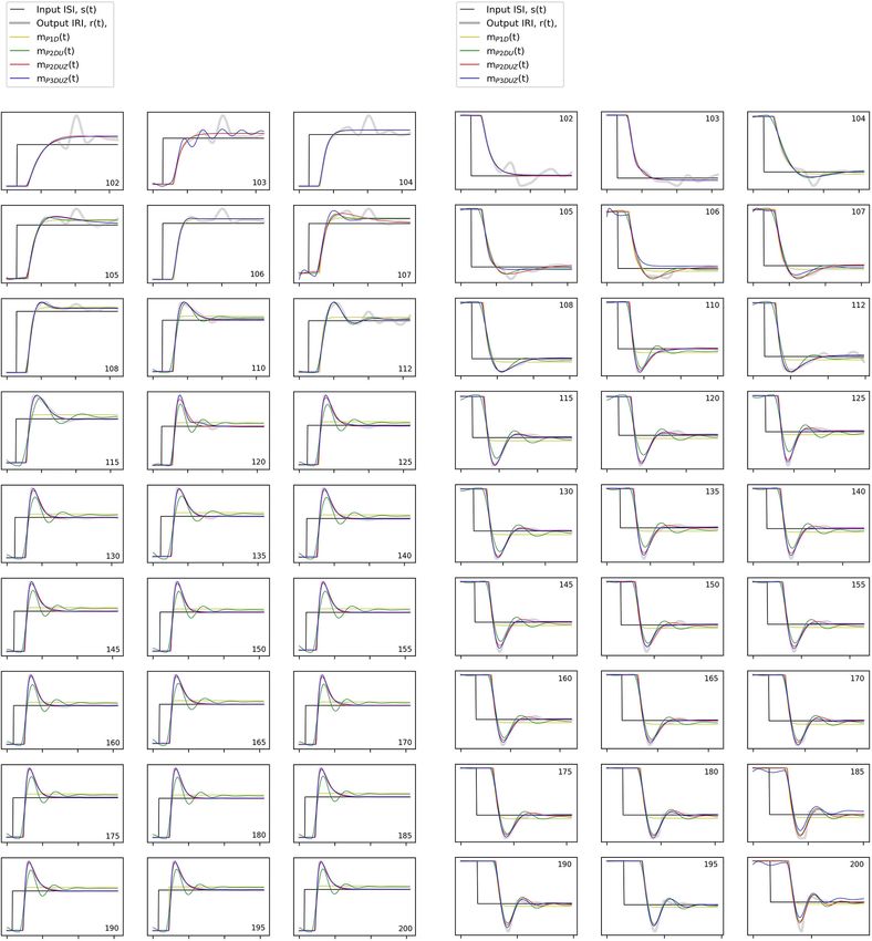
Darabi and Svensson                                                                                            Tempo Step Response in Frequency-Domain

systems theory approaches, on the other hand, is less focused             The existence or the relative size of such an overshoot, as well
on the inner-workings of the systems, usually takes a black-box           as the time of adaptation, can be better formulated by a new
approach, and is concerned with the mathematical description of           set of parameters that are described in the frequency domain.
the observable synergies. Given that the focus of dynamic systems         This study will hence present a model that introduces a new
theory is on continuous, non-linear, and within-cycle coupling            set of parameters, which leads to a better understanding of
(Large, 2008), it has typically been used for continuous movement         the behavior. The new parametrization uses parameters such
tasks, such as circle drawing in sync with external stimuli               as frequency of oscillation and damping ratio and can account
(Todd et al., 2002; Repp, 2005). Comparing the results obtained           for such observable qualities in the time signals. To do so, we
from series of time intervals produced in discrete finger-tapping         introduce system identification as a new approach to model SMS
tasks with the spectral analysis of synchronization-continuation          as a dynamic system. The simple scenario here is demonstrated
experiment reveals that movements that are organized as a                 to study the response of the “system,” a human in an SMS task, to
series of discrete contacts are consistent with an event-based            a stimulus with a step-wise changing tempo.
timing model and require more explicit temporal control than                  As introduced above, we are dealing with a discrete task of
continuous movements such as the oscillatory motion of the hand           generating rhythmic impulses, but we take a continuous-time
(Delignières et al., 2004). Although dynamic systems theories are         approach as in dynamic systems theory. The difficulty in such
general enough to encompass both continuous and discrete forms            an approach to SMS, as reported by Michon and Van der Valk
of periodic movements, they have primarily been used to analyze           (1967), is that the discrete nature of typical tapping/clapping
continuous movement tasks (Repp, 2005). Moreover, when the                experiments obstructs the underlying continuous process from
temporal goal is defined externally (e.g., by a metronome), timing        manifestation. The goal is to determine such a continuous
initially requires an event-based representation but after the            process, while the task is discrete, and the inter-sample behavior
first few movement cycles, control processes become established           of the system is not accessible in our limited experimental
that allow timing to become emergent and continuous (Ivry                 setup. The behavior of a human subject is assessed merely
et al., 2002; Zelaznik et al., 2005). It is also shown that event-        at its input/output level and sampled only at the time of
based and emergent timing can coexist in a dual-task of discrete          performed onsets. We do not have access to intermediate
(rhythmic tapping) and continuous (circle drawing) (Repp and              data related to the behavior of the system between the two
Steinman, 2010). These observations imply that both continuous            onsets, such as electrophysiological monitoring of the brain
and discrete processes might be involved in discrete finger-              activity, brain imagery, or any other behavioral data collected
tapping tasks and point to the potential suitability of dynamic           from the subjects at a higher sampling frequency than the
modeling in tasks of discrete finger-tapping.                             frequency of the rhythmic SMS task. In this context, the term
    A central hypothetical notion in the dynamic modeling of SMS          inter-sample behavior relies on the assumption that there is a
is the “internal timekeeper” that keeps track of time intervals           continuous internal process, which is reacting to discrete events
of the perceived rhythm of a metronome, other musicians, or               (Wing and Kristofferson, 1973).
a self-paced rhythm. Many attempts at modeling SMS behavior                   To overcome the problem of unknown inter-sample behavior,
use this notion as a basis for models of phase or period error            we will first upsample the sampled data collected at the
correction processes by assuming a quantifiable correction of the         input/output level of the human subject such that the temporal
timekeeper interval that ultimately affects the generated output          signals of pulses can be viewed as continuous-time signals in this
(Michon and Van der Valk, 1967; Wing and Kristofferson, 1973;             analysis1 We will then use a dynamic systems approach with a
Mates, 1994; Thaut M. H. et al., 1998). Michon and Van der Valk           tool which, to our best knowledge, has not been applied in the
(1967) introduced regularly time-sampled analysis to SMS and              study of SMS: so-called system identification, which is a standard
dynamic modeling of rhythmic behavior. He proposed a time-                tool in cybernetics, control theory and systems theory.
order representation that transforms the data from an irregularly             In control theory, signal processing, and cybernetics, state-
sampled format to a regular time series, enabling discrete-               space models mathematically describe a physical system2 by a set
time analysis that is otherwise inapplicable. Such representation         of input, output and state variables. These models can be non-
has since been used by those taking an information-processing             linear if they do not satisfy the properties of superposition3 . They
approach to the dynamic modeling of rhythmic behavior (Wing               can also be time-variant, i.e., the state variables of the model
and Kristofferson, 1973; Mates, 1994).                                    can change over time. We will show in the result section “Event
                                                                          and Interval Variables and the Choice Between the Period Error
Approach in the Present Study                                             Correction and Phase Correction Process” that the system which
As reviewed in section “Study of Sudden Step Changes,” literature         we are trying to model shows non-linearity, e.g., halving the
on SMS research tends to describe the qualitative difference              step size of the input would not cause a halved output but will
between subliminal and supraliminal step-changes in terms of
the existence of, or the magnitude of, an overshoot in the output
                                                                          1
intervals. Furthermore, the time of adaptation has been used to             Our upsampled signals are still discrete-time signals, but the sampling frequency
                                                                          is high enough that a continuous-time analysis can be used.
describe this difference, either expressed directly as the time, or       2
                                                                            Such as a participant at a sensorimotor task.
in terms of the number of tap/tones that it takes for adaptation          3
                                                                            Superposition properties imply that the net response caused by two or more
to take place. Such a tendency reflects a tradition of studying           stimuli is the sum of the responses that would have been caused by each stimulus
the signals from SMS experiments merely in the time domain.               individually.

Frontiers in Physiology | www.frontiersin.org                         3                                              June 2021 | Volume 12 | Article 667859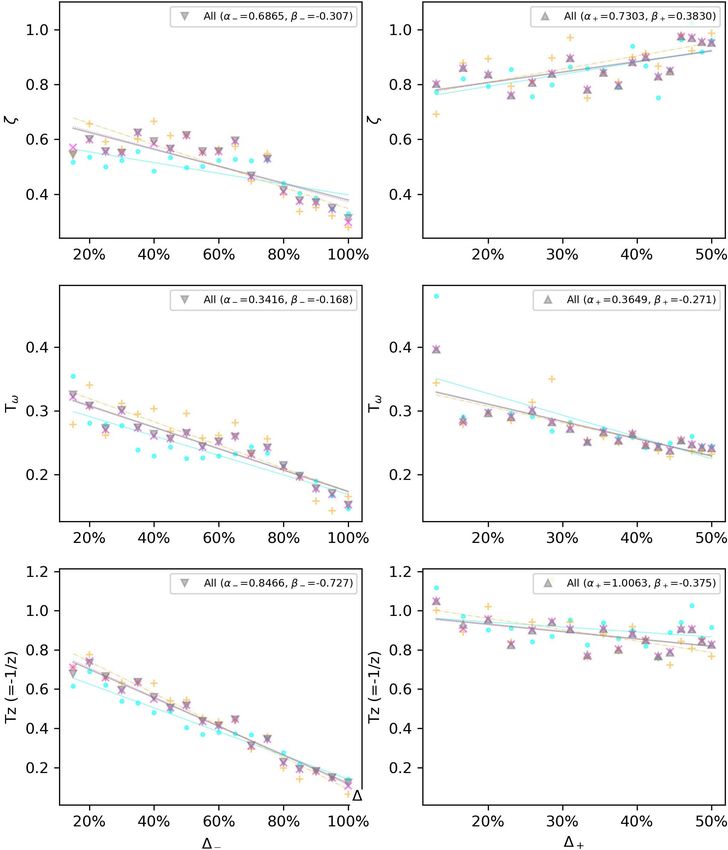
Darabi and Svensson                                                                                      Tempo Step Response in Frequency-Domain

instead change the behavior of the system. Therefore, our model            person. In other words, the successful production of a sequence
parameters can depend on the size of the step-change.                      of motor acts in synchrony with a rhythmic sequence of stimuli,
   The non-linear behavior of humans can be attributed to the              requires both synchronization of time events and minimization
finite thresholds of perceptual systems, as well as the human              of the discrepancy between the time intervals. Two internal
ability to learn and adapt to situations. This is because the human        error correction processes are usually defined in the studies of
tracker is more adaptive than a fixed linear system and takes              SMS corresponding to the two mentioned coordination tasks
advantage of the predictability in a tracking task. Additionally,          (Mates, 1994).
humans may not respond based on moment-to-moment input,                        A phase error correction process deals with the correction
as expected from a linear system, but would instead detect and             of synchronization error (or asynchrony), the time difference
respond to patterns when they are present (Jagacinski and Flach,           between the input stimuli and output response, Rij − Sij . A period
2018). This makes the identification of a fixed human transfer             error correction process, on the other hand, tries to correct
function impossible. Non-linear models could have been used to             the mismatch between the input and output intervals, IRI and
identify a control system vary, and many such possibilities exist          ISI, for example to minimize the value of rj − sj which is also
(Cloosterman et al., 2010; Strogatz, 2018).                                known as discrepancy. When the data is collected only at a
   However, as we will discuss in section “Results,” it is possible        final input/output endpoint, these processes are not uniquely
to view this particular non-linear system as a system that behaves         identifiable or separable from each other. We cannot tell to
as a linear, time-invariant system (LTI) for one particular input          which extent each process has contributed to the shifting of
signal. The system parameters will change gradually when the               the timestamp of a performed onset. Moreover, simulations
input signal changes gradually. This reduction, however, usually           have shown that their identified parameters can be highly
requires cutting down some dimensions of the data. In this                 interdependent (Schulze and Vorberg, 2002). Therefore, many
paper, we will model each participant at a fixed tempo step                studies have attempted to isolate only period correction by using
with an LTI system using the System Identification ToolboxTM               step changes, or phase correction by using phase perturbations
in MATLAB© . This toolbox uses an iterative prediction-error               (Repp, 2005; Repp and Su, 2013).
minimization method to update the initial model parameters                     The phase error correction process deals with precision in
to fit the given input and output data in a discrete-time state-           timing, while period error correction is in charge of the rhythm
space model. Using this method, we can identify the relationship           stability. There is a logical assumption that in a rhythmic SMS
between the input and output of a linear time-invariant single-            task, the latter is prior to the former, i.e., in the absence of a
input single-output (SISO) system.                                         stable rhythm during an SMS task, subjects would not prioritize
   Due to the noisy character of the data, quite a large number            timing accuracy. The adjustment of the interval variables (coping
of variations and repetitions were used, and this scale, together          IRI with ISI) is necessary for the synchronization of the
with the exploratory scope, limited the feasibility of a larger-           event variables. Mathematically speaking, in the presence of a
scale experiment. To get enough experimental data to use with              considerable discrepancy where interval variables are not in sync,
this method, then, a series of tests with finger-tapping tasks in          temporal synchronization between the event variables will be an
response to stepwise tempo changes for isochronous clicks as               accidental match and cannot last during the upcoming intervals.
stimuli were run with three participants.                                  Therefore, the phase error correction mechanism will fail to
                                                                           improve the timing accuracy in the absence of a stable rhythm.
                                                                           This consideration allows us to assume that in the presence of
Event and Interval Variables and the                                       considerable interval discrepancies, the phase correction process
Choice Between the Period Error                                            is shut down or negligible, and the period correction is the only
Correction and Phase Correction Process                                    active mechanism. The correction of asynchrony comes to the
Consider a one-to-one task for a person who tries to synchronize           play only after the subject has caught up with the tempo change.
responses Rj to a sequence of stimulus pulses Sj . Mates referred              It is thus reasonable that in this study dealing with a sudden
to the time instants of stimulus and response events as “event”            step-change in tempo, we will only model the period error
variables (“reading of a clock”), and used capital letters (Mates,         correction process.
1994). Temporal differences between two event variables were
then used for creating a new, derived set of data-points: interval
variables, symbolized by lower-case letters. For example, the
difference between two adjacent elements of Rj , is known as inter-        EXPERIMENTAL APPROACH
response interval or IRI, denoted by rj = Rj − Rj−1 . Similarly,
sj = Sj − Sj−1 is another interval variable called inter-stimulus          The current study uses the experimental approach from a
interval or ISI. It is also common in the SMS literature to use the        previous study, where a more detailed version of the methodology
term IOI to refer to either ISI or IRI, an interval variable whether       and the experimental setup is explained (Darabi et al., 2010).
it is from the stimulus or the response.                                   Here a somewhat brief description is given, with specifications
    In the SMS literature, two error correction processes are              of modifications from the previous study. A finger-tapping
thought to be underlying auditory sensorimotor behavior. For               task is given to a participant by presenting a click sequence
the successful accomplishment of a SMS task, both types of event           over headphones. The participant is given the task of following
and interval variables need to be in sync, as perceived by the             the click sequence stimulus by tapping on the space bar of a

Frontiers in Physiology | www.frontiersin.org                          4                                     June 2021 | Volume 12 | Article 667859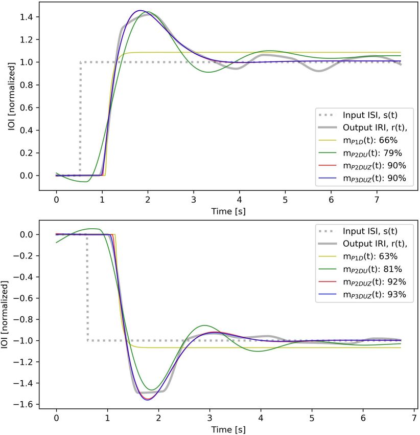
Darabi and Svensson                                                                                           Tempo Step Response in Frequency-Domain

MacBook Pro laptop computer. At some random point, the inter–             detected from user tapping, were recorded and saved in an XML
click period is changed suddenly, and the response to these               format for post-processing.
step changes is collected. In the previous study, 12 persons                  The stimulus in this study emulated a step-metronome, a
participated, and three different step changes were tested. Only          metronome jumping from one temporally regular (isochronous)
three participants were used in the current experiment, but               sequence of click sounds to another. Each session included a
a more fine-grained range of 27 step changes were tested,                 randomized number of 27–40 repetitions between two tempos.
each with 60–240 repetitions to reduce the effect of the noisy            Half of the repetitions, with a sudden decrease in tempo, were
character of the data.                                                    called positive steps due to an increase in the size of IOIs,
                                                                          and the other half, negative steps, had a sudden increase in
Black-Box Approach                                                        the tempo. The number of clicks before a step-change was
The internal workings of the synchronization mechanisms are               also randomized with the value changing between 10 and
still debatable due to the complex nature of the processes (Buhusi        30 throughout each session, to make the upcoming tempo
and Meck, 2005; Zatorre et al., 2007; Shadmehr et al., 2010).             change unpredictable for the participant. The participant would
In the current work, we will not try to break down the system             know that after a positive step, there would be a negative
into smaller parts or speculate about the inner workings of the           one with the same size, and vice versa, but could not know
tempo perception and action processes. Instead, we will take              when the change would occur. Each participant took part in
a “black-box” approach of treating the system as a whole and              twenty-seven different tempo step sessions changing between
assessing its behavior through a transfer function that describes         100 bps and a higher tempo (in a range of 102–200 bpm)
the mathematical relationship between its input and output. The           back and forth. Each participant, for each of the tempo steps,
system would then be a human performing a rhythmic task. The              took part in two to six sessions. Participants were blindfolded
input is the timestamps of onsets produced by the metronome               during all trials, and an assistant was present to monitor all
before and after a tempo change, and the output is the sequence           experiments (Figure 1).
of taps generated by the participant in response to that change.              In the previous study the influence of some factors was
The raw data must be processed before being used in our systems           found to be negligible, and as a consequence, those factors
modeling approach as described in section “Data Preperation.”             were kept constant in the current study. The effect of the
                                                                          lab conditions was studied in the previous work by carrying
Experimental Setup                                                        out the experiments in a normal quiet room as well as in
The sensorimotor task was finger-tapping in one-to-one to a               an anechoic chamber. The effects of this factor were not
regular sequence of heard impulses (via a headphone) and to keep          statistically significant, and thus an anechoic chamber did not
the synchrony by coping with a new tempo as quickly as possible           seem to be a necessity. Therefore, all trials in the current
after its sudden introduction. The auditory sequences of input            study were performed in a fairly damped and quiet room.
clicks of 3 ms long were generated by a computer application              Also, since other researchers reported that measurements
developed in Max/MSP [Computer software] (2018) and run                   using a keyboard might be subject to uncertainty in time
under MAC OSX Lion, and generating the output was done                    recording (Shimizu, 2002), in the previous study, we examined
by hitting the index finger on a MacBook Pro’s space button.              two means of hand-clapping and finger-tapping in similar
The same computer was used for all experiments, and the time              conditions and they led to indistinguishable results. Thus, only
resolution for the registration was 1 ms. The total closed-loop           finger-tapping was chosen as the medium of motor act in
delay was investigated by making the application respond to               this experiment.
the impulse sounds (clicks) that were created by triggering an                Among four methods of up-sampling investigated in the
auditory impulse detector instead of pushing the space button.            analysis of the recorded trials in the previous study, a so-called
The round-trip delay was 10 ms, and it was estimated that also            cubic Hermite interpolation (PCHIP) was chosen, in which each
with the keyboard input device, the delay was less than 10 ms. As         piece between two samples is a third-degree polynomial4 .
a result, the timestamps might have an error of maximum 10 ms.                Narrowing down the experimental factors enabled us to
    To perform the task, three trained participants from the              cover a larger number of tempo changes and to collect many
pool of 12 subjects in the previous study (Darabi et al., 2010)           more repetitions from fewer participants in the current study.
participated in the current experiment; two men (aged 31 and              Michon showed in his step change study that by averaging
33) and one woman (aged 32). The age of the participants                  the data over 10 tests, the noise of the inaccuracy was
was considerably below 66 and hence in the range that the                 effectively reduced to a negligible component (Michon and
errors of asynchrony are reported to be minimal (Drewing et al.,          Van der Valk, 1967). These numbers of repetitions were tried
2006). Subjects were not particularly trained as musicians but            out in the previous study but were not considered sufficient
were familiar with the test because of their participation in             to reduce the noise for the system identification methods
the previous study.                                                       used, especially for the small tempo steps. Small tempo steps
    The test was carried out in a quiet room. To decrease the             required more repetitions due to the higher ratio of jitter
uncertainty of the motor action, the subjects were instructed to          and other noise compared to the size of the step. The
use the wrist and not arm and to take an abrupt, pulsed release           number of repetitions collected for each step change, and each
of the downward force on the space key (Elliott et al., 2009). Both
arrays of impulse timestamps generated by the application, and            4
                                                                              https://www.mathworks.com/help/matlab/ref/pchip.html

Frontiers in Physiology | www.frontiersin.org                         5                                            June 2021 | Volume 12 | Article 667859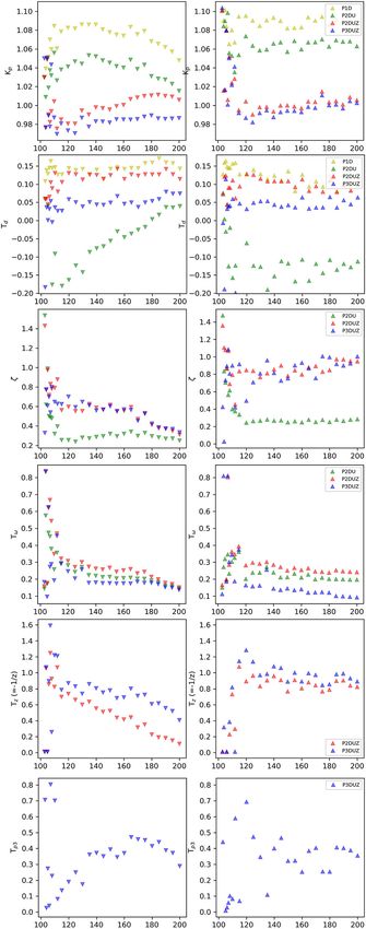
Darabi and Svensson Tempo Step Response in Frequency-Domain
FIGURE 1 | Illustration of the sensorimotor task.
participant, were hence between 60 and 240 depending on data must be converted to time signals that can be used
the tempo change. by this function.
To summarize the comparison of data collection to
the previous study, we chose a quiet but not anechoic
room as environment; used finger-tapping on a computer Breaking Down the Raw Data Into
keyboard for collecting the responses (clicks), and limited Repetitions
the experiment to three instead of twelve subjects. On Each session was recorded as a long sequence of timestamps,
the other hand, we expanded the number of tempo steps collected for repetitions of the same step-change. The sequence
from 3 to 27 for each positive and negative jump and was cut up into N sequences of single step repetitions with
also collected hundreds instead of dozens of repetitions an increase in the IOI (known as positive steps) as well as N
per each subject/tempo step to reduce the effect of sequences with a decrease in the IOI (i.e., negative steps). The
random variations and thereby improve the input data to index i represented the repetition number. Each of the repetitions
the model fitting. then contained a sequence of stimulus timestamps, Sij , for the
jth click of the ith repetition, as well as a sequence of response
timestamps, Rij for the jth tap of the ith repetition.
DATA PREPERATION The input sequences were cut so that they included two
stimulus clicks at the pre-step tempo, but contained various
The raw data collected from the experiment comprises of two numbers of clicks after the step. Since the corresponding response
sets of timestamps, of the stimuli “clicks” (which included sequences were cut at the same points, they also had different
a step-change in tempo) and the response “taps.” Since the numbers of post-step taps, but many enough that the responses
experiment deals with a one-to-one clicking task, there should were judged to come reasonably close to a stationary state after
nominally be the same number of click and tap timestamps. the introduction of the new tempo.
Our black-box approach uses a SISO system model, and the The raw data values, stimulus timestamps Sij , and the response
properties/parameters of that system which best fit the observed timestamps Rij were stored in two matrices, but given the
data points are found with the same tool as in the previous different lengths of various repetitions, the values after the ending
study: an iterative function in MATLAB’s system identification of shorter sequences were ignored.
toolbox called pem5 This function takes in two discrete-time The application produced the stimulus clicks as a metronome,
signals as input and output (see section “Data Analysis”). As so the stimuli Sij was supposed to be the same as the nominal
a first step of data preparation, the long sequences of clicks value, (=Ŝj ) for all i and j. Although a ± 1 ms “noise” was
and taps in each session are split up into shorter sequences, detected due to the temporal resolution of the timestamping of
one for each step-change in tempo. Then the timestamp the application.
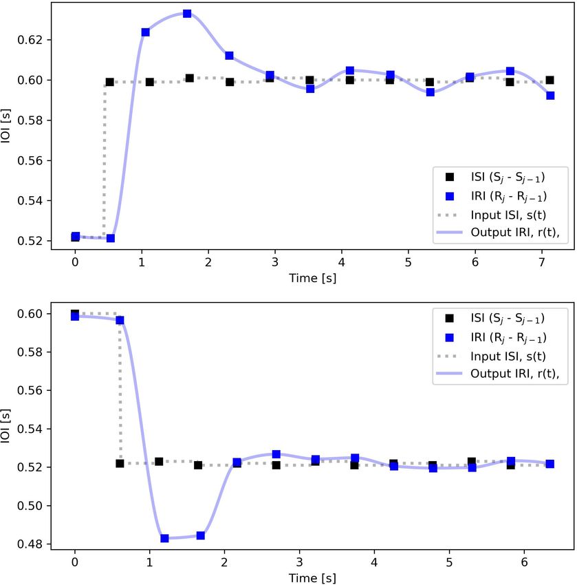
Figure 2 visualizes the matrix Rij by showing all repetitions
5
Prediction-error minimization https://ww2.mathworks.cn/help/ident/ref/pem. for one subject and one specific tempo step against the nominal
html values of Ŝj .
Frontiers in Physiology | www.frontiersin.org 6 June 2021 | Volume 12 | Article 667859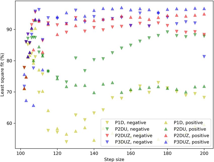
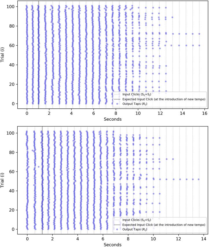
Darabi and Svensson                                                                                                        Tempo Step Response in Frequency-Domain

  FIGURE 2 | Visualization of the “event” variables for a specific subject/step size and for both positive/negative cases (Positive steps start in the range of
  103–200 bpm and with an increase in ISI/IRI, or a decline in tempo jump to 100 bpm. Negative steps begin with 100 bpm in the tempo and with a decrease in the
  IOI, jump to a higher tempo.). (Top) A positive step: 102 repetitions of one participant’s responses to a tempo change from 115 to 100 bpm (increasing ISI from
  0.522 to 0.6 s). The solid line shows where a stimulus onset was expected by the subject but occurred later due to the increase in ISI. (Bottom) A negative step: 103
  repetitions of the same participant responding to the tempo change from 100 to 115 bpm (decreasing ISI). The solid line shows that the first click after the tempo
  change, arrived slightly later than expected. The horizontal axis is transformed to time instead of tap index to mark at which timestamp the input and output onsets
  have occurred.

Treating Multiple Taps and Missed Taps                                                    It also happened that a participant performed the tapping
Sometimes a participant produced more than one tap for one                             too softly, such that the impulse detecting sensor would not
particular stimulus click. We had to make sure that the index j of                     register the created response (a space key in this case). By the
the output Rij was associated with the correct input Sij . Therefore,                  rule described above, a missing tap would cause the tap before or
for each repetition i we let only the tap closest to the nominal                       after itself to be assigned to two consecutive indices, Rij and Rij+1 .
Ŝj be indexed as Rij , which automatically excluded accidental                        An additional rule was then proposed that each tap should have
double-tap responses.                                                                  only one index, and in the case of Rij = Rij+1 , the closest nominal

Frontiers in Physiology | www.frontiersin.org                                      7                                             June 2021 | Volume 12 | Article 667859
Darabi and Svensson                                                                                                                Tempo Step Response in Frequency-Domain

stimulus to the tap’s timestamp, between Ŝj and Ŝj+1 , would define                       from the three participants, although still for the same step
its index, while the other one will be assigned a NaN value6 .                              size and direction.

Aggregating Response Data Over                                                              Calculating ISI and IRI Based on
Repetitions                                                                                 Aggregated Events
                                                                                            As discussed in section “Event and Interval Variables and
To convert matrices Sij and Rij to time signals that can be used
                                                                                            the Choice Between the Period Error Correction and Phase
by the model fitting algorithm, they should first be aggregated
                                                                                            Correction Process” concerning the nature of the SMS task at
over the repetitions i into vectors Ŝj and R̂j . This is trivial for the
                                                                                            hand, a sudden change in the interval, the focus would be on
input stimuli because the metronome timestamps vary negligibly
                                                                                            the period error correction and not the phase error correction
(±1 ms) over repetitions of the same step size, i.e., Ŝj ' Sij for any
                                                                                            process. This preference implies that instead of focusing on
i. Aggregating the matrix Rij into a representative R̂j array for all                       the properties of asynchrony between the input stimulus and
repetitions was done as follows.                                                            output response, Ŝj and R̂j , as aggregated event variables,
     First, after the re-indexing process described in section                              we are interested in the comparison between the values of
“Treating Multiple Taps and Missed Taps,” all response events,                              interval variables.
Rij , events that were assigned to the same index j were grouped in                            We can obtain the aggregated intervals by calculating the
the cluster. Rj = {Rij |∀i}                                                                 time difference between two consecutive values of the aggregated
     Next, outliers were removed within each cluster Rj .                                   events, r̂j = R̂j − R̂j−1 , and ŝj = Ŝj − Ŝj−1 . In the same way as for
Sometimes, a tap was mistakenly performed off-phase due                                     the event variables, interval values that deviated more than three
to a lack of attention or some other reason. Such taps that were                            standard deviations from each mean were considered as outliers
three standard deviations away or more from the mean of Rj ,                                and were discarded. This leads to the exclusion of another 2.4%
were marked as outliers and excluded. This led to the exclusion                             of datapoints in our dataset.
of around 1.7% of the responses/taps in our dataset7 .
     After grouping events and excluding outliers, a single value                           Transforming Index Number to Time
should represent all taps in each cluster, Rj , across the repetitions.
                                                                                            The aggregated ISIs and IRIs have so far been denoted with index
With the further considerations, the mean across repetitions i
                                                                                            number j. The next step is to transform the index number to the
for each Rj , was considered an acceptable candidate. We know
                                                                                            actual time of the events. This transformation is demonstrated
from the properties of asynchrony in rhythmic tasks that the
                                                                                            for one example of data points, as given in Table 1, showing that
distribution of the responses/taps is not always Gaussian around
                                                                                            ISIs (ŝj = Ŝj − Ŝj−1 ) can be described as a function of the time
an intended timestamp. Instead, the deviation from the intended
timestamp follows a power law with an exponent that depends on                              of Ŝj instead of the index j. Similarly, IRIs (r̂j = R̂j − R̂j−1 ) are
the rhythm frequency (Hänggi and Jung, 1995). Such a “colored                               expressed as function of the time R̂j 8 .
noise of asynchrony” is known as a 1/fB characteristic (Torre and
Wagenmakers, 2009). Because our trials were between 100 and                                 Upsampling the Signals
200 bpm, the maximum tempo was only twice the minimum,                                      The representation of the average IRI, R̂j , is smoother than any of
and for such a narrow range of inputs, the color of the noise will                          the individual repetitions, but is still a sequence of discrete events.
not have a significant influence on the calculation of the mean                             At this stage, we upsample the input ISI and output IRI data to
value. Therefore, we ignored such spectral aspects of the noise.                            signals with a considerably higher time resolution considerably
Furthermore, such 1/fB -noise is attributed to sustained attention                          higher than IRI or ISI intervals, by regularly inserting several
processes and fatigue in long trial sequences (Pressing and Jolley-                         8
                                                                                             These are functions of irregular time points and can be upsampled/interpolated
Rogers, 1997), but trials in our experiment were divided by                                 to be functions of regular time sample points, as described in the next section.
random breaks to reduce the effect of fatigue on the performance.
Distribution of asynchrony in other isochronous finger-tapping
experiments, which are performed on a similar limited range                                 TABLE 1 | One example of data points: the event times, Ŝj and R̂j , are for 5–6
of tempos, has also been shown to be Gaussian (Aschersleben,                                clicks/taps during an IOI step of 0.522–0.6 s (a tempo change from
2002). Based on these considerations, we assumed that we could                              115 to 100 bpm).
represent the set of all taps that correspond to the same tap index
                                                                                            j                 Ŝj                  R̂j                   ŝj                   r̂j
by their arithmetic mean, R̂j .
     Note that in the same way that we can aggregate one                                    0                  0                  0.011                   –                     –
participant’s data over all repetitions of the same step size                               1               0.521                 0.533                0.521                0.522
and direction, we can also aggregate over the pool of data                                  2                1.12                 1.053                0.599                0.521
                                                                                            3               1.719                 1.687                0.599                0.624
                                                                                            4                2.32                 2.311                0.601                0.633
6
  In the previous study, missed taps or claps were treated differently by inserting         5               2.919                 2.923                0.599                0.611
a hypothetical tap, i.e., dividing the IRI by two or a higher integer, if one or more
onsets were missed in a trial.                                                              Due to the small temporal uncertainty of the experimental system the clicks, Ŝj , do
7                                                                                           not occur exactly at an integer multiple of 0.522 s or 0.600 s. The interval variables,
  The expected value here is 0.3% since in a normal distribution 99.7% of
observations are supposed to fit within three standard deviations.                          ŝj and r̂j are computed as the difference between consecutive events.

Frontiers in Physiology | www.frontiersin.org                                           8                                                 June 2021 | Volume 12 | Article 667859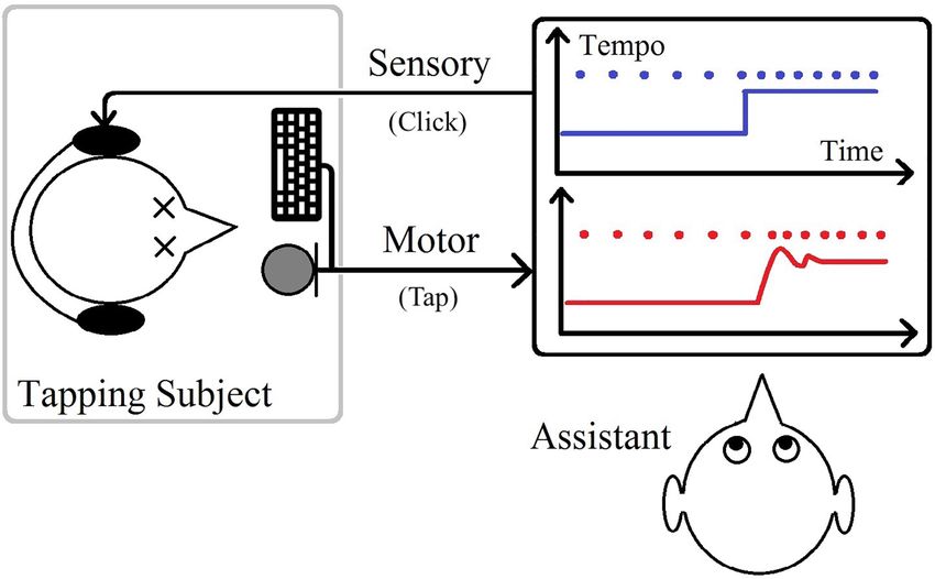
Darabi and Svensson                                                                                                        Tempo Step Response in Frequency-Domain

values in between these irregularly sampled data-points. This                               this condition, we scale signals s(t) and r(t), with the same scale
conversion assumes a short enough “time quantum” as the                                     factor, so that the input signal s(t) begins with 0 and ends with +1
indivisible unit of time that can be shared among all trials and                            for positive or −1 for negative steps, as seen in Figure 4.
will result in time signals with a regular, but higher frequency                               At this stage, the upsampled ISI and IRI signals are ready
of sampling, namely s(t) and r(t), respectively, for stimulus                               to be provided to the model fitting algorithm, which is the
and response, as seen in Figure 3. These new signals, although                              pem function in MATLAB’s System Identification ToolboxTM , as
still discrete-time signals, are quite smooth and represent the                             mentioned earlier. This function, by minimizing the normalized
hypothetical continuity of the internal timekeeper’s tempo with                             root mean square error (NRMSE), estimates parameters that
a higher regular frequency of sampling. In the previous studies                             produce modeled output curves to fit as close as possible to the
(Darabi et al., 2010), given the advice of sampling at ten times                            observed signals.
the dominant frequency of the system (Söderström and Stoica,
1989; Ljung, 1999) we chose the up-sampling frequency as 60 Hz.
Also, four different methods of interpolation were computed:                                DATA ANALYSIS
staircase, linear, cubic spline, and shape-preserving piecewise
cubic. Among these four, shape-preserving, or PCHIP, was                                    The stimulus input, s(t), and the response output, r(t), prepared
chosen to sample the output IRI in which the piece between two                              as described in the previous section, are functions of time, but
samples is interpolated with a third-degree polynomial. In this                             a Laplace transformation allows a formulation of the system
work, we use the same interpolation method for IRI outputs.                                 model in the complex frequency domain (the s-domain), as
For the input ISIs, we use a staircase interpolation with some                              described in section “Approach in the Present Study.” Such a
considerations as explained in section “Defining the Time of the                            model describes the transfer characteristics from the input to
Step-Change” on where to mark the timestamp of the step change.                             the output signals (Widder, 2015). The theoretical model that
                                                                                            describes the relationship between these two is written in the
Defining the Time of the Step-Change                                                        complex frequency domain as a function of s = σ + jω, after
During each click sequence, the participant will develop an                                 applying a Laplace transformation and in the form of a rational
anticipation of when the next stimulus click is supposed to come.                           transfer function, G (s) = A(s)/B(s), where A(s) and B(s) are
Therefore, a change in tempo will be detected differently in the                            polynomials (Trumper, 2004). The zeros of the system are the
two cases: either a new click arrives earlier than anticipated,                             roots of the numerator polynomial, A(s), and the poles are the
which happens in the case of a step-down in IOI (a step-up in                               roots of the denominator, B(s).
tempo), or a new click does not come at the expected time, which                               As mentioned in section “Approach in the Present Study,” the
occurs during a step-up in IOI (a step-down in tempo).                                      used software tool for fitting model parameters to experimental
    Due to this consideration, we define the start of a step                                data allows a model complexity up to three poles and one
differently for negative and positive cases. For the negative steps,                        zero. We will start with the simplest form of transfer function
where a click arrives earlier than anticipated, the timestamp of                            with a gain, one real pole, and a delay. Then we will add
that click’s arrival will define the start of the step-change9 For                          more poles and a zero to improve the fit. This step-by-step
the positive steps, however, we define the start of the step-change                         increase in the complexity reveals how each added parameter can
to be when the click was anticipated but did not arrive, instead                            capture a qualitative feature in the observed signals, and thereby
of the late arrival of the click, e.g., the dashed line in Figure 2                         improve the least-squares fit10 Fit ratios, normalized root mean
(bottom) instead of the third solid line where the first onset of the                       squared errors, for four different models are given in Figure 4,
new rhythm has arrived. This replacement is also visible in the                             for one example, which is the same case as in Figures 2, 3.
negative step of Figure 3 and will impact the quantity of the delay                         Figure 5 depicts how much the inclusion of each parameter
reported in the model fitting (see “Results” section).                                      would improve the fit ratio across all step sizes, where each step
    Also, the model fitting algorithm assumes that the response                             contains data merged from three participants. It is unsurprising
to a step input always happens sometime after the step has                                  that including more model parameters improves the fit; however,
occurred. Therefore, in order to make sure that the jump in                                 not all parameters play the same role. We will introduce them
the oversampled IRI signal certainly happens after the step-                                in this section and discuss them in the results section separately
change definition, we offset the IRI signal by adding a large                               to demonstrate how different parameters play different roles in
enough processing delay (1 s, for example). This value will                                 their qualitative impact on the shape of the signal by adding
later be subtracted from all the delays estimated by the model                              features such as delay, oscillation, overshoot without a following
fitting algorithm.                                                                          undershoot, etc.

Normalization                                                                               The First Real Pole and a Time Delay
The model fitting algorithm assumes that all signals, input and                             (P1D)
output, have the value zero before the time zero. In order to satisfy                       We begin with a rational transfer function, G(s), that has a
                                                                                            proportional gain Kp and a time constant Tp1 . Typically, the
9
 This will translate to a setting of kind = previous in staircase interpolation
                                                                                            10
functions which simply return the previous value of the point (the initial ISI) until        Minimizing the sum of squared residuals in the comparison between the
the new stimulus arrives as seen in the negative step of the Figure 3.                      modeled and the observed signals.

Frontiers in Physiology | www.frontiersin.org                                           9                                       June 2021 | Volume 12 | Article 667859
Darabi and Svensson Tempo Step Response in Frequency-Domain
FIGURE 3 | Aggregated stimulus and response intervals over repetitions for the same subject/step size as Figure 2 and Table 1. ISI, ŝj = Ŝj − Ŝj−1 (), and IRI,
r̂j = R̂j − R̂j−1 (), are plotted as function of time instead of index number. The output r(t) is upsampled with the PCHIP algorithm and the input s(t) with staircase
interpolation, both at 60 Hz sampling rate. Note that for the positive steps (increasing IOI, decreasing tempo) the arrival of the oversampled input step is marked
slightly (This shift is only considered for positive steps where IOI increases. It is the same as the temporal distance between the solid line and the third dashed line in
Figure 2, which in seconds amounts to 60/endtempo(bpm)−60/starttempo(bpm)) earlier than the arrival of the first onset of the new rhythm.
output follows the input after some delay, so we also define a This system, which allows a single pole p1 and a transport delay
“transport delay” TD in the time domain which is represented by TD , is called P1D. As shown in Figure 4, this model cannot
an e−TD s term in the complex frequency domain11 . generate an oscillation, which leads to a low fit ratio of 66 and
63% for the positive and the negative examples.
1
GP1D (s) = Kp e−TD s (1)
1 + Tp1 s
Adding the Second Pole (P2DU)
−1 In the example of Figure 4, the output r(t) for the P2DU
p1 = (2) model shows an overshoot and a subsequent oscillation around
Tp1
the input s(t), whereas the P1D can not capture this quality.
11 Exhibiting an overshoot is a sign of an oscillatory system, which
Note that as mentioned in 3.7, before feeding the signals to the system
identification toolbox, we offset the output by adding an additional processing needs at least two complex poles, i.e., (1 + Tp1 s)(1 + Tp2 s) in the
delay. Hence, this value should be subtracted from the estimated value of the TD . denominator, where p1,2 = −1/Tp1,2 . This denominator term can
Frontiers in Physiology | www.frontiersin.org 10 June 2021 | Volume 12 | Article 667859Darabi and Svensson Tempo Step Response in Frequency-Domain
FIGURE 4 | Measured data, ISI and IRI, as well as output signals from simulations with the four models defined in section “Data Analysis.” The input s(t) and the
output r(t) amplitudes are normalized. In addition, a processing delay of 0.4 s has been added to the output signal, before the model fitting.
be rewritten in the form of a second-order polynomial, based on a If ζ < 1, then according to Eq. 4, poles will have imaginary values
period T ω (alternatively described by the frequency of oscillation and the system, known as underdamped12 will oscillate and
f ω ) and a damping ratio ζ: exhibit an overshoot. In overdamped systems (ζ > 1), both poles
are real, and the output will follow the input without oscillation.
1
GP2DU (s) = Kp e−TD s (3) The Zero (P2DUZ)
1 + 2ζTω s + (Tω s)2
If α < 1, a second-order oscillator such as P2DU, in addition to an
overshoot of the size α, also shows a subsequent undershoot of the
size of α2 , followed by an overshoot of α3 , etc. This is because this
ζ2 − 1
p
−ζ ± model only has a frequency of oscillation and a damping ratio,
p1,2 = (4)
Tω which causes the system to show a secondary undershoot of the
same peak ratio as that of the initial overshoot.
1 2π 12
Allowing a system to oscillate in pem function is simply achieved by including
Tω = = (5)
fω ω the letter U (for underdamped) in the name of the model.
Frontiers in Physiology | www.frontiersin.org 11 June 2021 | Volume 12 | Article 667859Darabi and Svensson Tempo Step Response in Frequency-Domain
FIGURE 5 | Fit ratios for four models (P1D, P2DU, P2DUZ, and P3DUZ), on data aggregated over three participants. Negative steps are depicted with (∨) and
positive ones with (∧).
In order to capture the more complex response (overshoot gain Kp , the delay TD , the first two poles represented by T ω and ζ,
without a following undershoot), we introduce a zero, an extra the third pole defined by Tp3 , and the zero defined by Tz . Table 2
term in the numerator of the transfer function (Trumper, 2004): shows the inclusion of these parameters in each model.
1 + Tz s
GP2DUZ (s) = Kp e−TD s (6)
1 + 2ζTω s + (Tω s)2
RESULTS
1
z=− (7)
Tz In this section, in order to describe the relationship between input
According to Eq. 7, any of the previous systems without a zero, ISI and output IRIs, we will estimate the model parameters of the
have Tz = 0 and can be thought as having an infinite z. As seen transfer function in the Eq. 8, i.e., gain
in both Figures 4, 5, introducing a zero can lead to a substantial Kp , delay TD , up to three poles defined by Tp1,2,3 , and one
improvement in the fit ratio. zero Tz . Their qualitative impacts on the shape of the response
signal, as well as their trends, as a function of step size will
The Third Pole (P3DUZ) also be discussed.
Finally, a third pole can be given by a third-order denominator;
multiplying the complex conjugate pair with another linear term
to achieve the most general form of the model: TABLE 2 | Model parameters to describe the relationship between ISI and IRI.
1 + Tz s Model P1D P2DU P2DUZ P3DUZ
GP3DUZ (s) = Kp e−TD s (8)
1 + 2ζTω s + (Tω s)2 (1 + Tp3 s)
Gain Kp Kp Kp Kp
1 P1,2 Tp1 Tω Tω Tω
p3 = − (9) P1,2 – ζ ζ ζ
T p3
Delay Td Td Td Td
According to Eq. 8 depending on the complexity of the model we Z – – Tz Tz
have up to six parameters to study in the “Results” section: the P3 – – – T p3
Frontiers in Physiology | www.frontiersin.org 12 June 2021 | Volume 12 | Article 667859Darabi and Svensson Tempo Step Response in Frequency-Domain
FIGURE 6 | The stimulus signal, s(t) (black), observed step response aggregated over participants, r(t) (thick gray signal), and modeled response for all models,
mP 2DU (t), mP 2DUZ (t), and mP 3DUZ (t) (thin colored curves). The axes are the same as in Figure 4 with a normalized unit step input. The numbers in the corner of the
charts represent the initial tempo for the positive steps (left) and the destination tempo for the negative steps (right) in bpm, while the base tempo is 100 bpm.
General Characteristics of Step stimulus step input, the thick gray curve depicts the observed
Response Signals in Time Domain aggregated response, r(t), and thin curves with the same color
Figure 5 depicts the normalized least square fit for 27 negative code as Figures 4, 5 show how each model produces the
and positive steps, aggregating over the three participants. We step response. We can observe that mP2DU (t), mP2DUZ (t), and
can see that moving toward more complex models improves mP3DUZ (t) can capture the overshoot due to the inclusion of two
the fit overall. complex poles (P2) and the letter U. All models include the letter
In Figure 6, corresponding time signals are shown for all D and thus capture the delay. The models P2DUZ and P3DUZ,
tempo steps aggregated over three participants, both negative due to the inclusion of a zero (Z), allow for a proportionally
(left) and positive (right). The black curve, s(t), shows the smaller undershoot after the initial overshoot.
Frontiers in Physiology | www.frontiersin.org 13 June 2021 | Volume 12 | Article 667859Darabi and Svensson Tempo Step Response in Frequency-Domain
As a general observation, the model parameters will vary
across step sizes. Such dependence indicates a non-linear system,
which is a common observation in SMS research (Schulze et al.,
2005; Bavassi et al., 2013). This non-linearity means that the
same LTI system, no matter its complexity, cannot account for
modeling a single participant’s SMS behavior in response to a
sudden step-change in IOI. However, toward the end of this
section, we will introduce one model that allows changing its
parameters with the change in step size, as a workaround for
the non-linearity problem. We will limit that model to the step-
changes of 12% or higher. This limitation is because despite
collecting more repetitions for smaller steps (in the range of 102
to 110 bpm13 , the response signals and their modeled curves in
Figure 6 still appear noisier than for the larger steps, as it can also
be seen with the lower fit ratios in Figure 5.
Figure 7 reflects a regime shift at around 112 bpm, especially
for the models P2DUZ and P3DUZ. The transition at this
tempo, which matches the threshold between the subliminal and
supraliminal steps, demonstrates that our “black-box approach”
that disregards the system’s inner workings, can still shed light on
how different brain structures may be involved in an SMS task,
and is in agreement with neurophysiological insights regarding
different correlates involved in adaptation to subliminal or
supraliminal changes.
Some previous behavioral studies indicate that period and
phase correction processes are separate behaviors, with the
former being a higher-level cognitive process, while the latter
an automatic and related to lower-level cognitive processes
(Repp and Su, 2013). Repp (2002); Repp and Penel (2002)
showed that period correction is under conscious control,
while phase correction can be diminished by conscious effort
although never shut off completely. Friberg and Sundberg (1995)
claimed that the occurrence of overshoot in response to a
step-change in tempo does not depend on the amplitude of
the step-change, but rather on the awareness that the step-
change has taken place. Schulze defined two linear models which
used a different terminology by calling the phase and period
correction respectively “asynchrony-based” and “interval-based”
and showed that even if an asynchrony-based model matches
the data qualitatively, to fit the data quantitatively, we need to
consider another, interval-based correction process that adjusts
the period, although, it can switch on and off during a trial
(Schulze et al., 2005).
There are also neuroscientific studies pointing to different
neural correlates of subliminal vs. supraliminal errors.
Bijsterbosch et al. (2011a,b) focused on the role of the cerebellum,
the part of the brain at the back of the skull controlling muscular
activity. Their fMRI imaging showed that the right cerebellar
dentate nucleus and primary motor and sensory cortices were
activated during regular timing and during the correction of
subliminal phase errors. The correction of supraliminal phase
errors led to additional activations in the left cerebellum and
right inferior parietal and frontal areas. They also showed that
FIGURE 7 | Gain (Kp ), delay (TD ), damping ratio (ζ), oscillation period (T ω ),
zero (TZ -values), and the third pole (TP 3 -values). The parameters of the
13 aggregated data over participants for negative (∨) and positive (∧) steps, as
Due to the higher ratio of jitter and other noise compared to the step size (section
“Experimental Setup”) while normalizing all steps to the same value (section reported by the relevant models.
“Normalization”).
Frontiers in Physiology | www.frontiersin.org 14 June 2021 | Volume 12 | Article 667859You can also read