Grid-Based Bayesian Filtering Methods for Pedestrian Dead Reckoning Indoor Positioning Using Smartphones - MDPI
←
→
Page content transcription
If your browser does not render page correctly, please read the page content below
Article
Grid-Based Bayesian Filtering Methods for
Pedestrian Dead Reckoning Indoor Positioning
Using Smartphones
Miroslav Opiela *         and František Galčík
 Institute of Computer Science, Faculty of Science, Pavol Jozef Šafárik University, Jesenná 5,
 041 54 Košice, Slovakia; frantisek.galcik@upjs.sk
 * Correspondence: miroslav.opiela@upjs.sk

 Received: 13 August 2020; Accepted: 15 September 2020; Published: 18 September 2020

 Abstract: Indoor positioning systems for smartphones are often based on Pedestrian Dead
 Reckoning, which computes the current position from the previously estimated location. Noisy sensor
 measurements, inaccurate step length estimations, faulty direction detections, and a demand
 on the real-time calculation introduce the error which is suppressed using a map model and a
 Bayesian filtering. The main focus of this paper is on grid-based implementations of Bayes filters
 as an alternative to commonly used Kalman and particle filters. Our previous work regarding
 grid-based filters is elaborated and enriched with convolution mask calculations. More advanced
 implementations, the centroid grid filter, and the advanced point-mass filter are introduced.
 These implementations are analyzed and compared using different configurations on the same
 raw sensor recordings. The evaluation is performed on three sets of experiments: a custom simple
 path in faculty building in Slovakia, and on datasets from IPIN competitions from a shopping mall in
 France, 2018 and a research institute in Italy, 2019. Evaluation results suggests that proposed methods
 are qualified alternatives to the particle filter. Advantages, drawbacks and proper configurations of
 these filters are discussed in this paper.

 Keywords: indoor positioning; smartphone; PDR; Bayes filter; advanced point-mass; grid-based filter

1. Introduction
      Pedestrian navigation in a building complex [1], guiding visually impaired visitors in a
museum [2], helping patients to find a ward in a hospital [3], navigating a drone in a warehouse [4],
positioning in a historical building [5], navigating a person on a wheelchair [6], orientating firefighters
in a unknown indoor environment [7], and navigating cars in a parking garage [8] describe application
examples of indoor navigation system including the indoor localization. The existence of various
use cases determines assorted requirements on a positioning system. Unlike the outdoor navigation,
there is no unique adopted solution, as GNSS signal (e.g., GPS) is generally not available indoors.
      Typically, an indoor localization system available to a large scale of users utilizes the smartphones
with embedded sensors. As an alternative for some use cases, standalone Inertial Measurement Unit
(IMU), consisting of accelerometers, gyroscopes, and magnetometers, is fixed on a human body, mostly
on the foot [9] or sensors are attached to a robot [10]. Smartphone-based implementations able to cope
with the sensor bias are demanded, as the sensors produce noisy and inaccurate measurements [11–13].
Unlike the robot navigation, a smartphone position may be less predictable leading to approaches for
an activity recognition [14,15] to distinguish a movement type (e.g, walking, standing, using elevators,
or escalators) or a smartphone placement (e.g., in hand, in a pocket, or near ear in calling mode).
These methods improve the location awareness and provide additional input for the localization

Sensors 2020, 20, 5343; doi:10.3390/s20185343                                      www.mdpi.com/journal/sensors
Sensors 2020, 20, 5343 2 of 31
system. Typically, methods for the classification problem of human activity recognition are based
on machine learning approaches, mostly artificial neural networks, e.g., long short-term memory
(LSTM) [16].
Some positioning approaches require an infrastructure in the building often including its
calibration and maintenance, e.g., solutions based on Bluetooth Low-Energy (BLE) devices [3],
Ultra-wideband (UWB) [17], existing Wi-Fi access points [18], or so-called pseudolites to transmit
signals detectable by GPS receivers [19]. On the other hand, an infrastructure-independent approach
called Pedestrian Dead Reckoning (PDR) [9] exploits human kinematics and incorporates processed
sensor measurements as detected steps, their headings, and a map model into the relative position
estimation. The technique is suitable for a fusion with other methods, e.g., PDR, Wi-Fi, and landmarks
(walk types) [20], or PDR and visual landmarks (lights) [21]. A Bayesian filtering probabilistically
estimates the system state and is able to deal with the uncertainty introduced by noisy measurements
making the PDR approach applicable.
In this paper, we consider a use case where a user is equipped with a smartphone with embedded
sensors. Precise floor plans are available and no additional building infrastructure or devices are
required. Evaluation experiments are situated in a faculty building, a research institute, and a shopping
mall. The main aim of the paper is to evaluate different implementations of the Bayesian filtering,
analyze the results depending on selection of their parameter values, and compare them with focus on
the localization accuracy.
This paper is organized as follows. In Section 2, a related work based on Bayesian filtering
and PDR is reviewed followed by the overview of our approach and comments on the Bayesian
filtering applied on indoor positioning. In Section 3, the basic grid-based filter [22] is referenced and
extended with the convolution mask calculation, and further elaborated to a so-called centroid grid
filter. Section 4 introduces the advanced point-mass filter which we applied on the indoor positioning.
This filter is able to reduce some drawbacks of other grid-based approaches. The evaluation (Section 5)
reveals observations in three buildings where the algorithms are analyzed offline with different
parameter configurations on the same measurements. Moreover, the evaluation is performed using
various configurations of the particle filter to provide a reference for other methods, and the paper is
concluded with the results discussion and recommendations for the parameters setting.
2. Solution Background and Related Work
The dead reckoning approach computes a current user or device position from the previously
estimated position. Considering pedestrians, it is called pedestrian dead reckoning (PDR). Bayes filters
probabilistically estimate a state of a dynamic system using noisy measurements obtained up to the
current time of the estimation [23]. The Bayesian approach has found numerous applications in various
fields. In [24], a list of selected domains is proposed including, but not limited to, target tracking,
computer vision, robotics, speech enhancement and recognition, machine learning, financial and time
series analysis, and fault diagnosis. The Bayesian filtering and the PDR are two core components
of the proposed system. The PDR approach estimates a new user location and the Bayes filtering
technique incorporates the map model and deals with the uncertainty caused by noisy measurements
and inaccuracies introduced by PDR, e.g., inaccurate step length estimation.
2.1. Pedestrian Dead Reckoning and Bayesian Filtering Formulation
The PDR method calculates a position relative to the current estimation. When a step is detected,
the succeeding location is calculated from the sensors measurements, which may be expressed
as follows,
h iT
positiont = positiont−1 + Lt sin(θt ), cos(θt ) (1)
where θt is the heading and Lt is the length of the step detected at the time t.Sensors 2020, 20, 5343 3 of 31
Imperfect smartphone sensors producing noisy measurements are not capable of indicating the
accurate state (considering the indoor positioning, it is the user position and possibly other parameters,
e.g., the direction or the velocity). The uncertainty introduced by measurements is modeled by Bayes
filter, which represents the state at the time k ∈ N by a multivariate random variable xk . The belief
is a probability distribution over xk . The aim of the filter is to sequentially estimate the conditional
probability density function (pdf) p(xk |z1:k ) of the state xk given the sensor data as measurements
z1:k = {zi , i = 1, . . . , k} for the discrete-time stochastic system:
x k = f k ( x k −1 ) + w k , k = 1, 2, . . . (2)
zk = hk (xk ) + vk , k = 1, 2, . . . (3)
where xk ∈ Rnx is a vector representing the system state and zk ∈ Rnz is a vector representing the
measurements at the time k. Vector functions fk : Rnx → Rnx and hk : Rnx → Rnz are known and
wk ∈ Rnx , vk ∈ Rnz represent known, mutually independent zero-mean state, and measurement
noise, respectively. The solution of the filtering problem is given by the Bayesian recursive relations
consisting of two stages: the prediction and the correction:
Z
p(x |z )= p(x |z ) p(x |x ) dx (4)
| k {z1:k−1} | k−1{z 1:k−1} | k{zk−1} k−1
prediction prior pdf transition
predicted pdf evaluation
z }| { z }| {
p(xk |z1:k−1 ) p(zk |xk )
p(x |z ) = Z (5)
| k{z 1:k} p(xk |z1:k−1 ) p(zk |xk )dxk
correction (posterior pdf)
| {z }
normalizing constant
At the prediction stage, the pdf is distributed and spread according to the transition model
(Equation (2)), which brings more uncertainty to the state estimation regarding the noise wk . For the
system state estimation xk at the time k, the measurements z1:t are required. Depending on the
available measurements, one can distinguish stochastic smoothing if t > k, stochastic prediction given
t < k, and stochastic filtering problem for t = k. The posterior pdf estimation is computed from the
prior pdf, the transition and the evaluation model according to Equations (2) and (3), respectively.
This recursive approach to the stochastic filtering enables sequential processing of the measurements,
which is suitable for the real-time position estimation. The initial system state is determined at the
time k = 0 with no available measurements p(x0 |z0 ) = p(x0 ).
2.2. Particular Tasks Associated to Pedestrian Dead Reckoning
Various particular methods should be implemented to support the system to serve as a
comprehensive indoor positioning system. We review and comment on a few of them, which form
the proposed solution, i.e., a step detection, a walk heading calculation, a step length estimation,
a vertical localization, and an initial position determination. A supplementary positioning method
(e.g., Wi-Fi fingerprinting), in the fusion with the PDR and map constraints, arranges the initial location
determination and may update the position estimation, as the PDR error is increasing with the number
of estimated positions using inaccurate Lt and θt values caused by noisy sensor measurements.
2.2.1. Initial Position
The PDR approach estimates a relative position based on a prior estimation. The initial information
regarding the absolute position is required for the localization accuracy. Gionata et al. [25] introduced
a navigation system for impaired wheelchair users. IMU mounted on a wheelchair provides sensors
measurements for PDR and QR codes are used as landmarks with the encoded absolute position.Sensors 2020, 20, 5343 4 of 31
Scanning a QR code may be more user-friendly approach compared to a manual position setup.
An outdoor–indoor transition may be detected using machine learning approaches [26]. When the
navigation route or the localization initialization starts at the entrance of the building, the initialization
with GNSS signal is possible.
Solin et al. [27] initialize the solution based on a first magnetometer reading. Together with other
methods, the model converges to a reasonable certainty within a few seconds. If the initial location is
unknown, it is possible to setup a stochastic model to represent the prior position as a list of positions
with corresponding probabilities. In multiple approaches, where so-called particle filter is utilized,
the particles are initialized at random positions with equal weights across the map [21,28].
2.2.2. Step Detection
The detection of a performed step invokes the process of a new position estimation. Typically,
the step is detected from acquired accelerometer measurements, and the applied method is influenced
by the technique of mounting or holding the device. When the sensors are fixed on the user’s foot,
the stance phase of the foot can be easily detected in measurements and the periodic zero velocity
updates (ZUPT) are performed to bound the error [29]. Zhang et al. [30] introduced a method describing
zero velocity detection with the hidden Markov model, and four states are used to describe the walking
motion. Radu and Marina [31] proposed a localization system called HiMLoc for pedestrians holding
their smartphones in hand or in a pocket. The authors reference three different types of step detection
methods from accelerometer measurements, i.e., peak detection searching for local maximum or
minimum in the acceleration magnitude, searching for acceleration values crossing zero value, and the
autocorrelation leveraging the repetitiveness of human walking. In that solution, the zero crossing
method was applied on smoothed data. Ho et al. [32] applied a fast Fourier transform to smooth the
data and proposed a set of step detection rules. Lee et al. [33] proposed a step detection algorithm
with the average accuracy more than 98.6% for any combination of considered step modes and device
poses. In the project FootPath [34], the steps are detected when the acceleration value falls by at least
a given number within a given time window. An additional timeout value prevents multiple steps
detection within the same executed step. Brajdic and Harle [35] evaluated the step detection and
counting methods for different smartphone placements, and they highlighted the fact that none of the
examined algorithm was 100% reliable.
2.2.3. Step Heading
The magnetometer, often in combination with the gyroscope and the accelerometer, provides
a framework for the device orientation detection. The measurements may have a drift, and the
overall accuracy is influenced by metals and electrical equipment in the building [36]. Kang et al. [37]
proposed an improved step heading estimation, where the drawback of the gyroscope is reduced by
magnetometer measurements and vice versa. Seo and Laine [38] in their approach determine the device
orientation and then count the steps, which enables dynamic changes in the way of holding the device
without any significant error in the step detection. Wu et al. [39] introduced a heading estimation
method based on a robust adaptive Kalman filtering, which incorporates measurements from the
accelerometer, gyroscope, and magnetometer. Moreover, they integrated a model to limit outliers in
the measurement data and to resist negative effects of state model disturbances. Ettlinger et al. [40]
observed systematic deviations present in the data obtained from sensors. Their research is focused on
an analysis of a measure for the reliability (so-called partial redundancies), i.e., how well systematic
deviations can be detected in single observations, and the behavior of partial redundancy by modifying
the stochastic and functional model of the Kalman filter.
2.2.4. Step Length Estimation
Vezočnik and Juric [41] provided an in-depth analysis of different approaches to the step length
estimation. All thirteen considered models are classified to one of four categories: step-frequency-based,Sensors 2020, 20, 5343 5 of 31
acceleration-based, angle-based, and multiparameter. The evaluation was performed for different
walking speed values and various device placements: pocket, bag, hand-reading, and hand-swinging.
Constants were classified either as universal for all tests or personal tuned for each subject. Experiments
using personalized constants gained better accuracy compared to the universal constants. However,
the process of constants determination is time-consuming, which may be avoided in some use cases.
For personalized constants, the accelerometer-based solutions outperformed the others. For universal
constants, the step-frequency-based models obtained the most accurate results. Model proposed by
Tian et al. [42] performed best for personalized and model proposed by Weinberg [43] for universal set
of constants.
2.2.5. Vertical Localization
The indoor environment introduces a few novel challenges compared to outdoor navigation
systems including the positioning and the path planning through multiple floors. Bojja et al. [44]
proposed a localization approach for vehicles and pedestrians, where the three-dimensional position is
estimated using the particle filter. However, most solutions utilize barometer measurements to detect
floor transitions or to obtain the altitude information. Moreover, the position estimation is performed
on a single floor. The activity recognition supports the floor change detection by determining the
transition method, e.g., stairs, escalators, or elevators. Detecting a less frequent activity, such as using
an elevator, may further serve as a landmark to reduce the localization error in PDR by providing
more precise ground truth information [20]. Different solutions were implemented for the activity
recognition, e.g., deep learning approach [45] or a decision tree proposed by Wang et al. [36], where at
the top level the elevator is identified based on a unique accelerometer data pattern. The variance
in acceleration measurements separates walking and stairs from escalator and stationary, which are
discerned using magnetometer values. Xia et al. [46] highlighted the fact that the height of a floor is
not always known. In their solution, multiple barometers were installed in the building to provide
reference pressure values. Pipelidis et al. [47] proposed a dynamic vertical mapping system using
crowdsourced sensor measurements.
2.3. Bayesian Filtering Methods
Indoor localization systems using PDR for the position estimation utilize the Bayesian filtering
technique to deal with the uncertainty accumulated by noisy sensor measurements. The error
is reduced by incorporating another source of information, typically the map model. Moreover,
the filtering may be applied to various particular problems, e.g., the step length model calibration [48]
or the activity recognition [49].
Bayesian relations (defined in Equations (4) and (5)) specify only the conceptual solution
of the filtering problem. Arulampalam et al. [50] provide an overview of the Bayesian filtering
and its implementations, i.e., Kalman filters, particle filters and grid-based methods. As stated
by Arulampalam et al., the belief distribution is approximated when certain assumptions for the
exact solution calculation are not true, i.e., the analytic solution is intractable. The optimal Kalman
filter assumes the posterior density at every time to be Gaussian and the optimal grid-based filter
requires the state space to be discrete with a finite number of states, that is not fulfilled in the indoor
positioning problem.
Considering the indoor localization, the Kalman filter and the particle filter are the most
frequent approaches. In general, the state computation using the Kalman filter or its derivatives
has smaller computational demands compared to other approaches. However, if a probability
density is non-Gaussian, the Kalman filter cannot describe it well. In ref. [51], the Kalman filter
was overperformed by the particle filter in case of an imperfect trajectory obtained using Wi-Fi or
with fewer available access points. Table 1 presents an overview of a few published approaches to
indoor localization using Bayesian filtering. Use cases and device configurations vary in different
solutions. Presently, most of existing solutions utilize smartphones equipped with sensors whichSensors 2020, 20, 5343 6 of 31
provide connectivity and accessibility to the localization system. The particle filter is widely used
Bayes filter implementation for the positioning. Nevertheless, different approaches for the system state
definition and a fusion with additional techniques are applied to achieve satisfactory results.
Table 1. A comparison of a few selected indoor positioning systems in terms of considered device,
Bayesian filtering implementation, state representation, and other techniques applied to increase the
localization accuracy.
Year & Publication Device Bayes Filter State Additional Techniques
2019, Lu et al. [52] chest-mounted particle filter position, scale, map matching
IMU heading correction
2019, Xie et al. [53] robot with unscented position, velocity, visible light
camera Kalman filter ratio value
2018, Fetzer et al. [5] smartphone particle filter 3D position, Wi-Fi, floor detection,
heading activity recognition,
navigation mesh
2015, Chen et al. [20] smartphone Kalman filter 2D position Wi-Fi, landmarks
2015, Xu et al. [54] smartphone particle filter 2D position luminaries
2014, Bojja et al. [44] smartphone particle filter heading angle; 3D map matching,
East, North and moving maps, on-board
vertical coordinates diagnostics in a vehicle
2013, Radu & Marina [31] smartphone particle filter position, activity classifier, Wi-Fi,
PDR component map, landmarks
(activity, distance &
compass deviation)
2012, Rai et al. [55] smartphone augmented 2D position, Wi-Fi, map
particle filter stride length,
heading offset
2.4. Solution Overview
The aim of this paper is to evaluate and compare different Bayesian filtering methods,
which probabilistically model the uncertainty introduced by noisy measurements. Even though
ideal approaches are not chosen for every particular problem, the analysis of the performance with
inaccurate parameters is conducive to the overall solution set-up, e.g., how to configure methods to
handle underestimated or overestimated step lengths. An overview of our approach is outlined in
Figure 1 with the description of chosen methods.
Figure 1. Solution Overview. The aim of the paper is to compare different Bayesian filtering
implementations.Sensors 2020, 20, 5343 7 of 31
• Smartphone sensors used for the step detection and the walk direction determination are the
accelerometer and orientation sensors, the magnetometer, and the gyroscope, depending on the
device. The barometer is utilized for the floor change detection. We consider only the handheld
smartphone or tablet with the user looking at the screen. Sensors measurements are obtained via
API provided by the Android operating system.
• Initial position is set manually for the evaluation purpose, as it is assumed to be known. However,
in deployed application it would be replaced by an approach, which is more user-friendly, such
as scanning QR codes strategically placed in the building or possibly using an additional method,
e.g., Wi-Fi fingerprinting. When a floor transition is detected, the initial position is set at the entry
point to the floor, e.g., elevator doors or a position at the top of stairs.
• Step detection is performed on accelerometer measurements, which are smoothed to reduce the
noise. A low-pass filter is applied for smoothing and zero-crossing method proposed in [22] is
executed to detect steps.
• Step heading is obtained using API provided by the operating system. Android operating system
calculates the device position from the accelerometer and a geomagnetic field sensor [56]. Bearing
values are filtered to reduce the noise.
• Step length estimation is predefined for the purpose of this paper and fixed for a single evaluation
path. One of the research questions is, how the system is able to handle underestimated and
overestimated step lengths. In this case, the step length may be calibrated for a selected user
instead of computing the value from measurement data.
• Floor detection transition is performed using barometer measurements. The current position is
estimated on a single floor. Locations of all stairs, escalators, elevators and other places, where
it is possible to change the current floor, are collected in advance. If the transition is detected,
the new user position is set to the appropriate location according to the prior position knowledge.
• Map model is semi-automatically generated from floor plans by labeling walls manually in the
image. Map model provides information whether a position is accessible in the building or there
is a permanent obstacle, e.g., walls, places behind walls, and outside the building.
• Bayesian filtering probabilistically estimates a dynamic system state, which is restricted to a
single floor. We compare different implementations of the Bayesian filtering in this paper.
• Position estimation is calculated from the Bayesian filtering state, where the place with the
highest belief value is denoted as the estimated position.
2.5. Indoor Positioning Using Bayesian Filtering
The indoor positioning can be designed as the Bayesian filtering problem, i.e., the transition and
the evaluation functions, the state and the measurement noise, the system state, and the measurement
vectors are required to be defined. Some of these settings are analyzed in this paper, as we considered
and tested multiple choices. Our research is focused on grid-based implementations of the Bayesian
filtering. The main drawback of such filters is the computational complexity, which is growing
exponentially with the number of dimensions [23]. Therefore, the system state is preferred to be
low-dimensional. The system state vector may consists of more parameters, e.g., velocity and direction,
as discussed later. In our case, the state is determined only by the 2D position:
xk = ( xk , yk ) (6)
where the xk and yk coordinates may be expressed as longitude and latitude, respectively. However, we
prefer to use integers with centimeter-level precision denoting a distance to the reference point in the
map. When a step is detected, the posterior system state xk is computed using recursive relations from
the state at the time k − 1. The current measurement vector at the time k may be expressed as follows,
zk = (θk , L, Amap ) (7)Sensors 2020, 20, 5343 8 of 31
where θk denotes the heading value in degrees and L is the detected step length. In our model,
we consider the same value of the estimated step length for all detected steps. The parameter Amap
represents the map model by storing information about the accessibility of positions in the building.
Many buildings are formed of regular corridors which are mostly parallel or perpendicular to each
other. The map model coordinate system is adjusted that the orientation of the corridors are west–east
or north–south. Heading values obtained from sensors are translated with regard to the map rotation,
i.e., θk = 0 denotes the direction along the y-axis of the respective floor plan instead of the direction to
the north. When a transition between floors is detected, the estimation model is reset (k = 0), a new
map model is loaded and the current initial state is set according to the entry position.
Transition (Equation (2)) is performed using the PDR relative position estimation (Equation (1)):
fk ( xk , yk ) = ( xk + L × sin(θk ), yk + L × cos(θk )) (8)
The state noise is a zero-mean white noise with the covariance matrix cov(wk ) = diag(σ2 , σ2 ). Different
standard deviation values σ are tested in our experiments.
Evaluation (Equation (3)) is based on the provided map model, as seen in this simplified function:
(
1 if ( xk , yk ) is accessible
hk ( xk , yk ) = (9)
0 if ( xk , yk ) is not accessible
Inaccessible positions in the building represent walls, restricted places, permanent obstacles, and,
in some cases, places outside the building or the map. However, determining the accessibility only
from the location vector is not sufficient in most approaches. The direct PDR transition from an
accessible point A to an accessible point B with a wall between them should be restricted. Related
indoor localization systems often incorporate the map model into the transition function. In ref. [5],
a navigation graph and a mesh approach are proposed. The transition is performed only along these
structures preventing the step transition to intersect any obstacle. In our approach, the transition is
accomplished with no restrictions, but at the evaluation stage, the accessibility is determined using
both positions—the current one and the previous position, from which the transition was performed.
Moreover, the evaluation depends only on the map model. Therefore in our implementation,
the measurement noise is omitted, i.e., vk = 0.
3. Grid-Based Filter
The grid-based filter applied on the indoor positioning, extended with some practical
improvements, is discussed in ref. [22]. For the purpose of this paper, the brief outline of the method
is introduced in accordance with the specified Bayesian filtering formulation and these methods are
further elaborated. The enhanced convolution mask computation and the centroid grid filter are
proposed as an extension to the referenced work.
3.1. Grid Design and Computation
A floor plan is tessellated into a regular grid consisting of Ns grid cells {xik : i = 1, . . . , Ns } or
Ns isolated points {x̄ik : i = 1, . . . , Ns }. Typically, x̄ik is a center of the grid cell xik . The probability
distribution is approximated at these points with associated weights wik , likewise the particle filter:
Ns
p(xk |z1:k ) ≈ ∑ wik δ(xk − xik ) (10)
i =1Sensors 2020, 20, 5343 9 of 31
In this case, the weight or the belief value of a point denotes the probability that the current position is
within the grid cell. Probability density after the prediction stage execution is expressed as
Ns
p(xk |z1:k−1 ) ≈ ∑ w̄ik δ(xk − xik ) (11)
i =1
where weights w̄ik are computed from the prior grid using the transition model:
Ns
∑ wk−1 p(x̄ik |x̄k−1 )
j j
w̄ik ≈ (12)
j =1
Weights in the posterior state are computed using the predicted weights w̄ik and the evaluation model
followed by the normalization
w̄ik p(zk |x̄ik )
wik ≈ j j
(13)
N
∑ j=s 1 w̄k p(zk |x̄k )
In Equation (12), the belief value is calculated using a convolution. Convolution masks depend on
transition and noise models and define how the probabilities are redistributed during the prediction
stage. Moreover, it is possible to precompute the masks for selected values of the direction and the
step length to reduce the computational demands during the state estimation. Convolution masks
j
are typically smaller than the entire grid since the transition probability p(x̄ik |x̄k−1 ) = 0 for all pairs of
points with the distance greater than a single step length plus the maximal noise value. Equation (12)
expresses the method that for every point in the posterior grid, the weight is calculated from the
set of points in the prior grid according to the mask. The reverse process may be beneficial for
the implementation, where the prior grid points are iterated in a loop instead of the posterior grid
points. It allows to omit the convolution execution for points with zero or negligible weights. In the
implementation, the evaluation (Equation (13)) is performed during the convolution, enabling to
improve the usage of the map model. Therefore, the accessibility of a grid cell is not determined only
by its position, but also as an accessibility of the transition, i.e., a grid cell T is accessible from a grid
cell S if all cells composing the path from S to T are accessible. The path is constructed using a line
drawing algorithm and precomputed for relative positions of any two grid cells in the mask. Moreover,
different grid structures were investigated in the referenced previous work, i.e., the regular square
grid and the hexagonal grid consisting of regular hexagons, where the distance between centers of two
adjacent grid cells is the same in all six directions.
To sum up a single iteration, when a step is detected, a convolution mask is loaded according to
the step length and the direction, the convolution is performed, the grid is normalized, and the new
position estimation is found at the grid cell (center point) with the highest belief value. The convolution
mask is applied on all grid cells with positive belief values, whereas the accessibility of the path between
a source cell and the target cell is verified.
3.2. Convolution Mask
Processing a detected step is performed using the convolution followed by the weight
normalization. An efficient convolution implementation iterates only over active prior grid cells,
i.e., grid cells with positive weight values. It is possible to define the threshold making the cells with
their associated weight under the threshold negligible and prevent them from the computation. In this
case, the threshold is set to 0. Weights in the posterior grid are computed in the loop using the formula
for a pair of indices i and t denoting the transition between these two grid cells:
−i i
wkt = wkt + mtα,L wk−1 h(i, t) (14)Sensors 2020, 20, 5343 10 of 31
where the index i denotes a point in the prior grid associated with the positive weight, i.e., i = {b ∈
{1, . . . , Ns } : wkb−1 > T } with the threshold T = 0 and the index t denotes the target point in the
posterior grid. The function h(i, t) returns the value one, if the grid cell t is accessible from the grid cell
i, and it is zero otherwise. The convolution mask Mα,L models the transition and the noise. The mask
j
for a given direction α and a step length L is expressed as Mα,L = {mα,L : j = − Nm , . . . , 0, . . . , Nm },
where the position with the index 0 determines the origin, i.e., the mask position associated with the
grid position where the mask is applied. The mask size 2Nm + 1 is selected to cover relative positions
j
of grid cells which are affected by the convolution, i.e., the values which are not 0. The value mα,L
represents the probability of the transition from the origin position (j = 0) to the relative position at the
index j. The value m0α,L encodes the probability of no movement. The construction of the convolution
mask is visualized in Figure 2. The step length and the direction are modeled using normal distribution
with the mean at the estimated step length or the measured step heading, respectively, and multiplied
j
by each other to form the value mα,L . The belief value of a mask grid cell is determined by the
cumulative distribution function regarding the bounds of the grid cell. The same approach is applied
for the mask computation on hexagonal grids, where only the bounds of a grid cell calculation differs
from the square grid. To reduce the computation costs, the masks can be precomputed and stored for
specified step lengths and headings. Measured and expected values for the length and the heading
are rounded. Therefore, one of stored masks is loaded and applied for the state calculation when a
step is detected. In our implementation, relative indices in the mask representing the shifts in the
grid are transformed in regard to the full grid size, as the two-dimensional position is encoded in a
single index.
Figure 2. The convolution mask computation. The green grid cell denotes the origin of the mask,
and the value for the yellow grid cell is computed using the cumulative distribution function for the
normal distribution of the step length or the heading, respectively. The left figure displays the bounds
for the step length and the bounds for the heading in the right figure.
A more accurate method for the mask computation is proposed in this work using two layers
of grids. A coarse grid is identical with the previous method, where the space is tessellated into grid
cells with assigned weights. A fine grid layer has the same structure, but consists of more points,
as the distance between two adjacent points is smaller, i.e., the density of points is several times greater.
The probability density value is calculated at these fine grid points denoting the probability of the
transition from the origin to the given point. The coarse grid weights are expressed as a sum of
probability density values of all fine grid points within the single coarse grid cell. The weights are
normalized in the grid.
The mask in this approach is defined as a distributing mask, i.e., a value in the mask denotes the
probability of the transition from the origin to the given target point. Therefore, the convolution is
iterated over the prior grid and the mask determines how the belief value is distributed in the posterior
grid. The opposite method defines a mask value as the transition probability from the given point
to the origin. The step processing algorithm iterates over the posterior grid cells. This approach is
beneficial for the centroid grid filtering method introduced in this paper.Sensors 2020, 20, 5343 11 of 31
3.3. Centroid Grid Filter
A rule of thumb for a real-time indoor positioning application is that the position estimation
should be completed before the succeeding step is detected. Therefore, it is possible to improve the
localization accuracy by increasing the number of all grid points only to some extent. The localization
error is influenced not only by noisy inputs, but also by the discrete approximation of the continuous
state space in grid-based filters. The proposed approach assumes two grid layers, as in the introduced
mask computation. The weight is associated with the coarse grid cell, but the estimated position is not
always represented by the center of the grid cell, as visualized in Figure 3.
Figure 3. Purple arrow represents the step from the red point. Left figure shows that in the grid filter,
the next position is estimated at the green point in the grid cell center point instead of the true location
denoted by the blue point. In the centroid grid filter (figure on the right), the next position is chosen
from the set of fine grid points.
Formally, the coarse grid Gk consists of Ns grid cells Gk = {xik : i = 1, . . . , Ns }. Every grid cell xik
is associated with the weight value wik (Equation (10)), and the position estimation expressed as x̄ik
i
0 = { x0 : i = 1, . . . , N }. In this approach, the x̄i is not the center of the
and a fine grid of Nu points Gk,i k u k
0 . A so-called centroid of a coarse grid cell xi is labeled
grid cell, but selected from the set of points Gk,i k
j
0 , i.e., ci = j such that x̄i = x0 . The fine grid
as cik , and it denotes the corresponding index in the Gk,i k k k
S Ns
covering the entire state space is defined as Gk0 = i=1 Gk,i0 . Coarse and fine grid point positions are
fixed. Therefore, it is sufficient only to compute weights and select centroids for all coarse grid cells in
the posterior state, when a step is detected. Belief values are computed for all coarse grid cells using
the formula
Ns
i −t
wkt = ∑ wik−1 m0 α,L,cik−1 h(i, t) t = 1, . . . , Ns (15)
i =1
where h(i, t) is zero, if the transition from the grid cell i to the target coarse grid cell t is not
i −t j
possible and one otherwise. The value m0 α,L,ci is obtained from the mask Mα,L,c0 = {m0 α,L,c : j =
k −1
− Nm , . . . , 0, . . . , Nm }. The mask is constructed similarly to the aforementioned method using the fine
−t
grid, but the value miα,L,c denotes the probability of the transition from the centroid position at index i
to the origin, i.e., the target grid cell where the weight is computed. Masks are created and stored for
all combinations of considered step lengths L, step headings α and centroid indices c. The index of the
fine grid position within a coarse grid cell is selected using the weighted centroid approach:
N
∑i=s1 wik→t cik→t
ctk = t = 1, . . . , Ns (16)
wkt
i −t
where wik→t = wik−1 m0 α,L,ci h(i, t) is the summand expressed in Equation (15), i.e., wkt = ∑iN=s1 wik→t .
k −1
The value cik→t is precomputed and stored with the mask values determining the target fine grid index,
when the probability is transformed from a coarse grid cell i to the cell t.Sensors 2020, 20, 5343 12 of 31
To reduce the computational demands on the convolution, the masks are precomputed for selected
step lengths and directions. The real values from sensors are rounded and the corresponding mask is
applied on the filtering. The weight calculation (Equation (15)) is not performed for all coarse grid
cells. Active coarse grid cells with positive weight values in Gk−1 are iterated, and reachable cells in
Gk , which are not yet computed, are considered as target cells t. Another technique to improve the
speed of the posterior state computation is resetting the negligible values. Values lower than a selected
threshold are set to 0 in the correction phase before all weights are normalized. A less efficient but more
stable method keeps a predefined maximum number of active grid cells. Therefore, weights for all
cells, sorted by belief values, extending the limit are set to 0. The drawback of such methods is that in
some scenarios, especially with incorrect step length estimations, the knowledge of a position may be
lost and a recovery method must be implemented based on the history of estimations or other inputs
to avoid the uniform distribution of the probability over the entire map as discussed in the evaluation.
To sum up a single iteration, the process after a step is detected is the same as for the
aforementioned basic grid filter. However, the convolution phase differs. In our implementation,
all grid cells in the prior grid with positive values are iterated to mark grid cells in the posterior
grid which are reachable, i.e., the distance is within the mask size. The convolution mask is loaded,
the belief values are computed, and the centroid of the particular target cell in the posterior grid is
calculated. Optionally, grid cells with positive values in the posterior grid are sorted and reset based
on the given maximum number of active grid cells.
4. Advanced Point-Mass Filter
The advanced point-mass filter (APM) is a numerical approach to solve Bayesian recursive
relations based on the approximation of a continuous state space by one or multiple grids of points.
Like grid-based filters, the belief values are computed only on these points. However, the floating
grid technique used in APM enables the grid to transform and rotate according to the non-negligible
support of the pdf. Therefore, the APM filter is able to focus on the relevant positions with the higher
resolution, similarly to the particle filter, but with all advantages provided by the grid approach
and the convolution computation. In ref. [57], the full algorithm of the APM is introduced by
Šimandl et al. and it is compared with the particle filter applied on a nonlinear state estimation
problem. In their evaluation, lower computational demands are achieved without a loss of accuracy.
The applicability of the method on the indoor localization problem is investigated in this paper.
Specifics of the algorithm and the implementation are commented. Moreover, the evaluation includes
the the parameter configuration discussion and the comparison with other filters, especially in terms
of the accuracy.
4.1. Algorithm Overview
A basic scheme of the adapted method for the two-dimensional indoor localization problem is
proposed in this paper. A density function p(xk |z1:k ) at the time k is represented by a grid of Nk points
Gk = {xik : xik ∈ R2 , i = 1, . . . , Nk }, by a set of volume masses for grid cells Dk = {∆xik , i = 1, . . . , Nk },
and by a set of belief values at the points Pk = Pk|1:k = {wik : wik = p(xik |zk ), xik ∈ Gk }. A set of belief
values after the prediction stage of the Bayesian filtering is defined as P̄k = Pk|1:k−1 = {w̄ik : w̄ik =
p(xik |zk−1 ), xik ∈ Gk }. A grid cell volume mass is for the two-dimensional localization interpreted as the
area covered by the grid cell. The APM filter assumes the points to be the centers of the corresponding
grid cells.
Initialization: Define an initial state represented by a grid G0 , D0 , and P0 for the prior pdf p(x0 ). Then,
proceed to following four steps for k = 1, 2, 3 . . . .
(1) Filtering: Compute values of the approximate filtering pdf at points of the grid Gk using the
Equation (5) for the correction stage, for i = 1, . . . , Nk :
wik = c− 1 i i
k w̄k pvk ( zk − hk ( xk )) (17)Sensors 2020, 20, 5343 13 of 31
where pvk (zk − hk (xik )) denotes the evaluation p(zk |xk ) from the Equation (5) and the
N
normalization constant is defined as c− 1
k = ∑i =1 ∆xk w̄k pvk ( zk − hk ( xk )). As the measurements
k i i i
depend only on the map model, its integration is included in the algorithm during the convolution
phase likewise the grid-based filter implementation. Therefore, the filtering step consists only of
the normalization
w̄i
wik = N k (18)
∑i=k1 ∆xik w̄ik
Optionally, the negligible belief values may be reset to zeros. In this step, the grids are split,
if necessary in the multigrid version of the filter and the weights of the grids are computed.
(2) Time Update of Grid: Transform the grid Gk to a grid Hk+1 = {yik+1 : i = 1, . . . , Nk } with the
equal number of points using the PDR system dynamics:
yik+1 = fk (xik ) i = 1, . . . , Nk (19)
where fk denotes the state transition function defined in (8). In general, the transition function
is allowed to be nonlinear and the grid Hk+1 may have different structural properties than Gk .
The grid Hk+1 integrates the state transition noise and covers the support of pdf, i.e., the relevant
area, where positive belief values would occur. The local predictive mean and the covariance
matrix is calculated and the grid merging for multigrid APM is executed, if necessary.
(3) Grid redefinition: Redefine the grid Hk+1 to obtain a new grid Gk+1 = {xik+1 : i = 1, . . . , Nk+1 }
for the state xt+1 , incorporating the state noise wt , with the same structural properties as the
original grid Gk . The number of points Nk+1 may be different than the value Nk in the preceding
state. Compute the number of points, Dk+1 , and rotate the grid according to a computed
transformation matrix.
(4) Prediction: Compute values of the approximate predictive pdf at the new grid Gk+1 using (4) for
i = 1, . . . , Nk+1 :
Nk
∑ ∆xk wk pwk (xik+1 − yk+1 )
j j j
w̄ik+1 = (20)
j =1
j
where pwk (xik+1 − yk+1 ) denotes the transition pdf p(xk+1 |xk ), xik+1 ∈ Gk+1 and yik+1 ∈ Hk+1 .
Predictive belief values are calculated using the convolution from corrected belief values Pk and
grid points determined by the grid Hk+1 .
Figure 4 visualizes a computation of a posterior state. The grid Gk is transformed to the grid Hk+1
and redefined to the posterior grid Gk+1 . The time update stage relocates all points from the prior grid
according to the PDR, the measured step heading, and the estimated step length. The posterior grid is
further redefined. Moreover, the process includes a calculation of the grid size and the point density in
the grid. In the prediction phase, new values for the belief set are computed, based on the prior grid
and the map model or measurements in general.
The filtering phase consisting of the normalization and the prediction in the form of the
convolution are present also in other grid filters implementations. However, the PDR translation
according to the step length estimation and the direction is included in the convolution mask for grid
filters. The APM separates these two parts, i.e., all points composing the grid are translated along the
vector in the second phase and the convolution models only the noise and is direction-independent.
Moreover, the grid points are constructed for the following state (in the third phase) unlike other grid
filters where point positions are fixed.Sensors 2020, 20, 5343 14 of 31
(a) Single step detected. (b) Time update. (c) Grid redefinition. (d) Prediction.
Figure 4. A step is performed from the yellow to the blue point. Circles denotes true pdf (a) which is
approximated by a grid. Grid Hk+1 (blue points) is obtained from the original grid Gk (b), which is
later (c) redefined to the grid Gk+1 (black points). The convolution sets belief values (d) in respect to
the prior grid and the measurements (red area represents a wall; a larger point width denotes a larger
belief value).
4.2. Method Features and Implementation Remarks
The computational time for the APM filtering technique may be reduced by applying particular
methods for the grid manipulation. An outline of adopted features of the framework (anticipative and
boundary-based approaches, thrifty convolution, and multigrid representation) is provided with
additional implementation remarks.
The convolution is a demanding operation of the APM filter and should be implemented smoothly
to enable the algorithm to provide position estimations in real-time. The thrifty convolution derives
only significant points in the transformed grid Hk+1 for points in Gk+1 based on the their distance,
i.e., points too far from each other are not included in the convolution computation as the belief gain
would be negligible. Moreover, the map accessibility is verified for all grid points. Convolution masks
cannot be stored as for other grid filters. However, the calculated values from normal distributions
may be cached to speed up the convolution.
The so-called anticipative approach determines the number of grid points and the point mass
(corresponding to the grid cell size in grid filters). These calculations are performed during the
third phase of the algorithm (grid redefinition). However, for larger scenarios it may be necessary
to limit the number of all points. Therefore, this approach is not fully utilized in this work.
Moreover, the boundary-based approach detects the area of interest where the grid should be placed.
This process is similar to storing active grid cells as proposed in grid-based filters to be considered in
the convolution.
To support multimodal distributions, the multigrid representation is introduced by authors of the
APM. The basic algorithm is extended with a grid splitting and a merging process. During the first step
(filtering) and after the normalization, the grids are examined and a grid is split to two disjoint grids
if there are separable areas on the marginal densities. This process should be performed repeatedly
until there is no grid to split. However, we found it sufficient to perform this step only once. Two grids
may be merged after the PDR transition in the second step (time update of the grid). The criterion
for merging two overlapping grids is the Mahalanobis distance between a point and a distribution
(mean and covariance matrix are computed for all grids). This method is not covering all situations
but it is convenient for the purpose of the method. Moreover, weights are assigned to all grids and
these grids are handled independently. The grid weight is computed as a multiplication of the belief
sum and the point mass.
5. Evaluation
Proposed methods are evaluated on a few sets of experiments. Raw sensor measurements are
recorded for each subject with a handheld device while they are walking along the predefined path.
Checkpoints with known positions for measuring the localization accuracy are denoted on the floor
and indicated in data manually by the user during the experiment. The evaluation of differentSensors 2020, 20, 5343 15 of 31
approaches and configurations is executed afterwards using an offline simulation tool on the same
sensor measurements. More than 3000 simulations are considered for this evaluation. The core input
files, map models, results, and visualizations are published [58].
Various scenarios were used to support the expectations of proposed approaches and to expose
different aspects of the methods. Three different venues are locations of the evaluation. A simple
path to verify methods and configuration was set in a faculty building in Slovakia. To evaluate the
performance in a real scenario, we used datasets from a competition held at IPIN 2018 (International
Conference on Indoor Positioning and Indoor Navigation) in a shopping mall in France (the dataset [59]
and the work in ref. [60] available) and IPIN 2019 competition in a research institute in Italy [61].
The main research focus is on the localization accuracy. The overall accuracy may be increased
using additional approaches, e.g., Wi-Fi fingerprinting. In the evaluation, we address the following
research questions.
• How robust are Bayesian filtering implementations to the inaccurate step length estimation?
• What is the difference in the localization error using introduced versions of grid-based filters and
various configuration values?
• What values of standard deviation are suggested to use for considered filters?
• What configuration and version of the particle filter gives the best results and can be chosen as a
reference for overall evaluation of considered filters?
• What is the stability of considered filters in terms of using rotated maps or the
experiment repetition?
• What is the overall accuracy of the proposed system? Is the performance at the satisfactory level
in a new building without any further calibration?
Followed sections discussing the evaluation is organized as follows. A summary of considered
methods and scenarios provide an insight to the evaluation background. A methodology and a
general performance of the proposed system are outlined followed by the discussion of the parameter
configuration for grid based filters, the particle filter, and the advanced point-mass filter. The overall
localization accuracy is evaluated on IPIN competition datasets and the discussion of these results
concludes the observations for all considered filters.
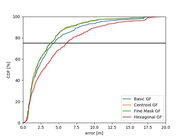
5.1. Considered Methods
The following approaches are applied to estimate user locations especially on predefined
checkpoints. These methods are compared with focus on the localization accuracy, computational
demands, and their reliability.
1. Basic Grid Filter (basic GF) with a two dimensional square-shaped grid introduced in the
referenced publication and recapitulated in Sections 3.1 and 3.2.
2. Fine Mask Grid Filter differs from the basic GF in the mask design. The fine mask construction
proposed in the Section 3.2 is used for the convolution to estimate the posterior grid state.
3. Hexagonal Grid Filter utilizes hexagonal grid cells as proposed in the referenced research and
the Section 3.1.
4. Centroid Grid Filter with square-shaped grid cells where the position is not attached to the
middle point but is chosen from a set of points, as introduced in Section 3.3.
5. Particle Filter (PF) is selected for the comparison with grid-based filters. The SIR particle filter
implementation introduced by Teammco and Xie [62] is adapted for the evaluation.
6. Advanced Point-Mass Filter (APM), proposed by Šimandl et al. [57], is applied on the indoor
localization according to the Section 4.
Various configurations of selected methods are investigated. Noise models, i.e., step length and
direction standard deviations, and step length estimations are analyzed for all six methods. The accentSensors 2020, 20, 5343 16 of 31
is on the step length selection. Other parameters are tested with various step lengths to demonstrate
how the solutions deal with underestimated and overestimated values.
5.2. Scenarios
The first set of experiments was conducted in the faculty building (Park Angelinum 9, 04001
Košice, Slovakia). Nine checkpoints were placed at positions which support the analysis of the
localization error (Figure 5). The scenario consists of a straight walk and two 90◦ turns performed in a
few steps. Six subjects, mostly students, were asked to walk along the path and mark the checkpoint on
the Lenovo tablet held in hand. Before the experiment, their approximate step lengths were calculated
using the distance measurement after 20 executed steps (one subject performs the experiment twice),
which are expressed in cm {79.1, 91.1, 79.1, 84.7, 66.4, 78.0, 84.7}. The main purpose of this scenario is
to evaluate and observe methods and parameter settings in the controlled environment with known
subjects and devices supported by external camera recordings. The path is 85 m long and its simple
layout, compared to other experiments, makes it suitable for proving concepts, observing tendencies in
data, and comparing the influence of some parameters, instead of the complex verification of methods.
Figure 5. Checkpoint positions in the first scenario. The route starts on #1 and ends on the marker #9
consisting of more than a hundred steps on average. Every subject traveled 85 m along the markers in
the ascending order.
The main part of the evaluation is performed on data acquired in the shopping mall Atlantis le
Centre near Nantes, France (Boulevard Salvador Allende, 44800 Saint-Herblain, France). Organizers of
the IPIN 2018 competition provide the dataset useful for the competition preparation but also for the
more objective comparison with other solutions. The dataset consists of testing and validation logfiles.
An additional single track for the off-site competition was not used in this evaluation. Every logfile
contains between 10 and 24 landmarks where the ground truth position is known and the localization
accuracy is computed. These files were used to calibrate parameters of the considered methods and to
systematically find the most suitable configuration, especially the major part of testing was executed
on the fourth testing path labeled by the logfile T04_01 in the referenced dataset, which is more than
220 m long. The validation logfiles are prepared to score the positioning system. Only a few best
configurations based on the testing logfiles are executed in the validation process. The validation
measurements were obtained on 6 routes. Every file from 13 available sensor logs has from 10 to
17 ground truth positions. Details regarding the device and the user are unknown.
In the same shopping mall, the on-site competition was held during busy hours on a Saturday
afternoon. The more comprehensive path was 800 m long with 70 ground truth locations andYou can also read