Land-Use Change and Future Water Demand in California's Central Coast - MDPI
←
→
Page content transcription
If your browser does not render page correctly, please read the page content below
land
Article
Land-Use Change and Future Water Demand in
California’s Central Coast
Tamara S. Wilson 1, * , Nathan D. Van Schmidt 2 and Ruth Langridge 2
 1   U.S. Geological Survey, Western Geographic Science Center, P.O. Box 158, Moffett Field, CA 94035, USA
 2   Social Sciences Division, University of California, Santa Cruz, 1156 High Street, Santa Cruz, CA 95064, USA;
     nvanschm@ucsc.edu (N.D.V.S.); rlangrid@ucsc.edu (R.L.)
 *   Correspondence: tswilson@usgs.gov

 Received: 1 August 2020; Accepted: 9 September 2020; Published: 14 September 2020

 Abstract: Understanding future land-use related water demand is important for planners and
 resource managers in identifying potential shortages and crafting mitigation strategies. This is
 especially the case for regions dependent on limited local groundwater supplies. For the groundwater
 dependent Central Coast of California, we developed two scenarios of future land use and water
 demand based on sampling from a historical land change record: a business-as-usual scenario (BAU;
 1992–2016) and a recent-modern scenario (RM; 2002–2016). We modeled the scenarios in the stochastic,
 empirically based, spatially explicit LUCAS state-and-transition simulation model at a high resolution
 (270-m) for the years 2001–2100 across 10 Monte Carlo simulations, applying current land zoning
 restrictions. Under the BAU scenario, regional water demand increased by an estimated ~222.7 Mm3
 by 2100, driven by the continuation of perennial cropland expansion as well as higher than modern
 urbanization rates. Since 2000, mandates have been in place restricting new development unless
 adequate water resources could be identified. Despite these restrictions, water demand dramatically
 increased in the RM scenario by 310.6 Mm3 by century’s end, driven by the projected continuation of
 dramatic orchard and vineyard expansion trends. Overall, increased perennial cropland leads to a
 near doubling to tripling perennial water demand by 2100. Our scenario projections can provide
 water managers and policy makers with information on diverging land use and water use futures
 based on observed land change and water use trends, helping to better inform land and resource
 management decisions.

 Keywords: land use; land cover; land change modeling; water demand; water use; California;
 Central Coast; state-and-transition simulation modeling; LUCAS model

1. Introduction
     Water availability and human land use are inextricably tied [1]. In water limited regions, available
freshwater supplies can often dictate land use intensity. However water withdrawals and diversions to
support land uses, especially for irrigated agriculture, directly impact freshwater supplies [2]. Adding to
the complexity are the associated feedbacks between land use, climate, and water supplies. Human land
use has been attributed to widespread increases in average global temperatures, contributing to global
warming [3–5], losses in species diversity, [6–9], changes in water quality [10–12], and groundwater
depletion [13]. Land use models have been widely used to examine future land-use change and water
resource assessments in global [14,15], national [16], and regional analyses [17–19]. Understanding
potential future land-use related water demand in a region serves as a first step in assessing prospective
outcomes and associated mitigation strategies to address potential vulnerabilities.
     California exemplifies these issues with water, arguably the state’s most contentious resource.
The state boasts one of the most productive agricultural regions in the world, worth ~$50 billion [20],

Land 2020, 9, 322; doi:10.3390/land9090322                                            www.mdpi.com/journal/land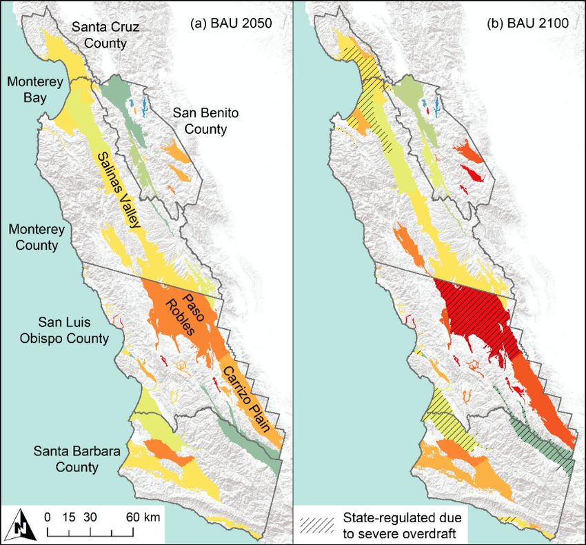
Land 2020, 9, 322                                                                                   2 of 21

which consumes between 60–80% of all water supplies, while residential and industrial consumption
is roughly 17% [21–23]. Surface water is over allocated, estimated at 400 billion cubic meters, 5 times
the average annual runoff [24]. The state’s Mediterranean climate is highly variable, characterized by
long-term droughts and atmospheric river flooding events [25], contributing to inter-annual water
supply uncertainty. Moreover, water demand is highest in the dry, summer months. A statewide
extreme drought from 2012–2016 led to water shortages, increased reliance on groundwater pumping,
and subsequent well drying [26], and contributed to saltwater intrusion in some groundwater
basins [27–29].
      Efforts to plan for water resource sustainability are more challenging now than ever, as these
drought and flood events increase in frequency and intensity due to a changing climate [3,30,31].
While the state has long experienced periodic droughts, many climate projections show increased
drought occurrence in coming decades [3,13,32–35]. Reduced surface water during drought often leads
to increased groundwater pumping in the state [36–38]. Recent work also projects a 25–100% increase
in extreme wet/dry events by century’s end, despite only modest changes in mean precipitation [39].
Such extreme events, combined with increased evaporative water demand due to climate warming,
as well as future population growth and agricultural expansion, will likely contribute to even greater
water demand, posing additional challenges to an already unsustainable situation. This may lead to a
pivotal juncture where water demand exceeds sustainable supply.
      Oversight of California’s groundwater has historically been limited. While surface water
withdrawals require permits, groundwater pumping has gone largely unregulated and is managed
locally [40]. Several legislative attempts have been made to incentivize groundwater management and
to better integrate land use in water supply planning. In 1992, AB 3030 passed, and was modified in 2002
by SB 1938, providing procedures and incentives for local agencies to voluntarily develop groundwater
management plans [41,42]. In 1995, Senate Bill (SB) 901 required that local governments conduct water
supply assessments during the environmental reviews for large projects (above 500 housing units) [43].
In 2001, Senate Bills 610 and 221 required local land use authorities to demonstrate long-term water
supply availability before approving new, large development projects [44,45]. Despite these restrictions,
none of these laws regulated groundwater pumping. By 2014, rapidly falling groundwater tables
combined with ongoing extreme drought led the state to pass the Sustainable Groundwater Management
Act (SGMA; AB 1739, SB 1168, and SB 1319) [46–48]. Passage of SGMA marked the first time,
local agencies were required to regulate and sustainably manage groundwater resources of critically
over-drafted groundwater basins. The implementation of SGMA is ongoing, with local agencies
actively designing their groundwater sustainability plans. However, many of these agencies lack the
ability to quantify sustainable groundwater yield driven by future land use related water demand.
      California’s Central Coast is an ideal system for examining the linkages between land use change
and land use driven water demand over time and exploring the long-term impacts of water laws and
policies on this process, as well as impacts on groundwater supplies, and resource and community
sustainability. The region has major agricultural and residential areas that are entirely reliant on local
groundwater. There is limited imported surface water, primarily in San Benito and Santa Barbara
counties, and groundwater overdraft (extraction exceeding recharge) occurs in an estimated 40% of
basins in the region [49]. Many of the coastal aquifers have seawater intrusion, exacerbated by the
recent droughts, rendering local groundwater unsuitable for drinking or irrigation [27–29]. Many of its
valley floors overlie groundwater basins and support extensive agriculture, while the vast majority
is largely undeveloped natural land, creating the potential for substantial new development. It is
home to some of the wealthiest and poorest communities in the state, including several disadvantaged
communities (annual median household incomes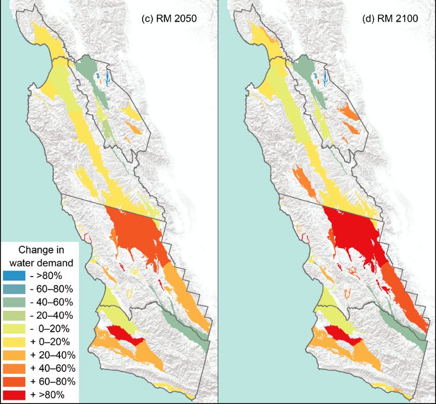
Land 2020, 9, 322 3 of 21
To assess the trajectory of land use driven water demand for California’s Central Coast and
explore whether the 1992–2001 water laws and policies were correlated with the pattern of demand for
the region, we ran two scenarios based on historical, empirical datasets of land use changes sampled.
The first was a business-as-usual (BAU) scenario fit to land use change rates from the entire historical
period, 1992–2016, while the second, recent-modern (RM) scenario only sampled from 2002–2016 rates
(i.e., after the second set of laws were put in place in 2001). We simulated projected land use change
and associated water demand for the years 2001–2100 at 270-m across 10 Monte Carlo simulations
across these two scenarios. Our model was based on the Land Use and Carbon Scenario Simulator
(LUCAS) [18,19,53–57], a stochastic, spatially explicit state-and-transition simulation model. Spatial
patterning of land use change was parameterized using local zoning datasets, identifying where land
change would and would not occur giving current zoning ordinances and local mandates. Our goal
was to understand the region’s unique potential water demand, assisting local water resource and land
managers in understanding the impacts of past policies to better identify and mitigate for possible
future vulnerabilities as they continue to develop and revise new groundwater sustainability plans
for SGMA. While SGMA is too new to definitively determine its impact on future water demand,
viewing an unregulated future with and without existing policy provides an important baseline for
more targeted mitigation planning.
2. Materials and Methods
The LUCAS state-and-transition simulation model (STSM) [19,54–56] was developed and modified
for our study region. An STSM is a stochastic, Markov chain, empirical simulation model used to predict
how defined variables transition between different specified states over a specified timeframe [58].
An STSM can also track age structure enabling age-dependent transitions as well as age-based triggering
events. STSMs have been widely used to simulate landscape level vegetation change [59] and changes
in land use and land cover (LULC) over time for assessing LULC scenario impacts on population and
carbon dynamics [53–55], protected areas [57], and future water resources [19,56]. The STSM divides
the landscape up into spatially discrete simulation cells, each with assigned state classes (i.e., LULC)
and transition types. Each state class has pre-defined transition type pathways, allowing or preventing
cells to move between different state classes over time. What follows is a description of the model
parameterization steps for the Central Coast region of California. For more comprehensive information
on STSMs, see Daniel et al. [60]. All modeling for this study was done using the ST-SIM software
application, which can be downloaded free of charge from APEX Resource Management Solutions
(http://apexrms.com). All model parameters are available as (1) a Microsoft Excel file and (2) a database
containing all model inputs and outputs (http://geography.wr.usgs.gov/LUCC/) and in the ScienceBase
USGS catalog (https://www.sciencebase.gov/catalog/).
We held three stakeholder meetings with individuals from regional municipal governments,
water agencies, and community groups while developing our models. Meetings were held at the start
of model development, the midpoint, and when presenting a draft version of the final model results.
Stakeholders provided information on local spatial planning datasets that were assimilated into the
models (see Section 2.5) as well as interpretation of results in the context of local concerns about water
sustainability and land use.
2.1. State Variables and Scale
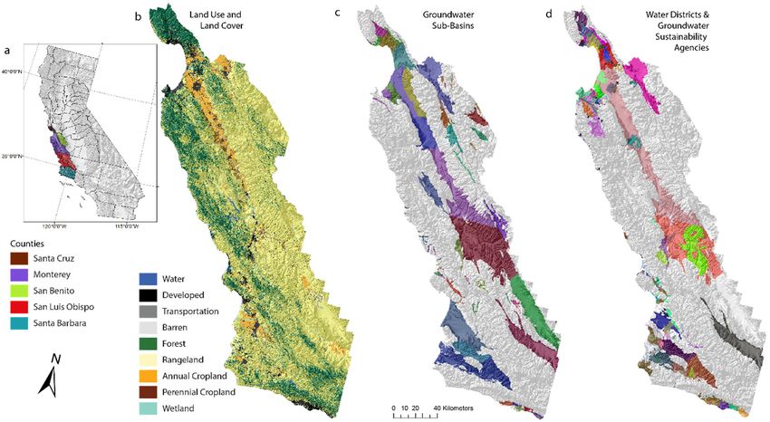
The current study area encompasses 28,534 km2 of the 5-county region in California’s Central
Coast (Figure 1a), covering Santa Cruz, San Benito, Monterey, San Luis Obispo, and Santa Barbara
Counties. The region was divided into 270-m × 270-m simulation cells (391,421 total cells). Each cell was
also assigned an initial LULC state class (Figure 1b) and three additional spatial identifiers including its
(1) county, (2) groundwater sub-basin (Figure 1c; n = 61) [61], and (3) water service agency(s) (Figure 1d;
n = 107), which are described below. Scenario simulations were initiated in 2001 and run through
the year 2100. The model tracks changes in state class, age, time-since-transition, and state attributes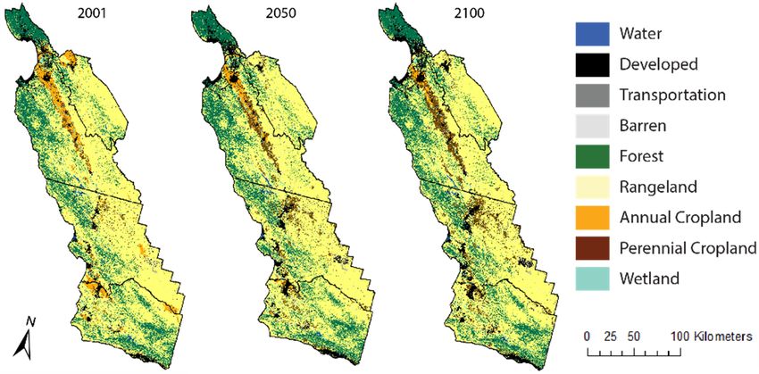
Land 2020, 9, x FOR PEER REVIEW 4 of 21
Land 2020, 9, 322 4 of 21
and run through the year 2100. The model tracks changes in state class, age, time-since-transition,
and state attributes (i.e., water demand). For each scenario simulation, we ran 10 Monte Carlo
(i.e., water demand). For each scenario simulation, we ran 10 Monte Carlo iterations to capture model
iterations to capture model variability and uncertainty in our projections.
variability and uncertainty in our projections.
We utilized the National Land Cover Dataset 2001 (NLCD01) [62], as our initial state class
We utilized the National Land Cover Dataset 2001 (NLCD01) [62], as our initial state class
conditions, modified for our study region were as follows: (1) all four developed classes were
conditions, modified for our study region were as follows: (1) all four developed classes were collapsed
collapsed into a single developed class and urban core areas defined per [63]; (2) the three forest
into a single developed class and urban core areas defined per [63]; (2) the three forest classes were
classes were combined into a single forest class; (3) the woody and emergent wetlands classes were
combined into a single forest class; (3) the woody and emergent wetlands classes were combined
combined into a single wetlands class; (4) the agriculture and hay pasture classes were combined into
into a single wetlands class; (4) the agriculture and hay pasture classes were combined into a single
a single annual agriculture class; (5) we used data from Sleeter et al. [55], for the 2001 perennial
annual agriculture class; (5) we used data from Sleeter et al. [55], for the 2001 perennial agriculture
agriculture class, described in more detail below; and (6) the “Developed-Roads” class from
class, described in more detail below; and (6) the “Developed-Roads” class from Landfire’s Existing
Landfire’s Existing Vegetation Cover 2001 was used to designate a transportation class [64], (Figure
Vegetation Cover 2001 was used to designate a transportation class [64], (Figure 1b). All datasets were
1b). All datasets were resampled from 30-m to 270-m and re-projected into a NAD 1983 California
resampled from 30-m to 270-m and re-projected into a NAD 1983 California Teale Albers map projection.
Teale Albers map projection.
Figure1.1. California’s
Figure California’s Central
Central Coast
Coast Study
StudyArea
Areaincluding
including(a)
(a)counties,
counties,(b)
(b)land
landuse
useand
andland
landcover
coverinin
2001, (c) groundwater sub-basins, and (d) aggregated water district and groundwater sustainability
2001, (c) groundwater sub-basins, and (d) aggregated water district and groundwater sustainability
agencyjurisdictions.
agency jurisdictions. Complete
Complete lists
lists of
of regions
regions included
included in
in (c)
(c) and
and (d)
(d)located
locatedin
inthe
theSupplementary
Supplementary
Materials Tables S1 and S2, respectively. The base map is from the U.S. Geological Survey’s
Materials Tables S1 and S2, respectively. The base map is from the U.S. Geological Survey’s National National
Map Atlas [65].
Map Atlas [65].
TheNLCD01
The NLCD01does doesnotnotcontain
containaaperennial
perennialorchard
orchardand andvineyard
vineyardclass.
class. We
Weused
usedaa2001
2001 perennial
perennial
cropland cover
cropland cover map
map [55],
[55], which
which generated
generated orchard
orchard and and vineyard
vineyard cover
cover using
using aa gradient
gradient boosting
boosting
machinealgorithm
machine algorithmframework.
framework.Any Any NLCD01
NLCD01 pixel
pixel classified
classified as agriculture
as agriculture whichwhich overlapped
overlapped the
the 2001
2001 perennial
perennial cover cover estimate
estimate was classified
was classified as perennial
as perennial cropland.
cropland.
Thewater
The wateragencies
agenciesmap map(Figure
(Figure1d)1d)was
wascreated
createdby bycombining
combiningthe theGroundwater
GroundwaterSustainability
Sustainability
Agency (GSA)
Agency (GSA) Service
Service Area
Area dataset
dataset [66],
[66], and
and thethe Water
Water Districts
Districts dataset
dataset [67].
[67]. Because
Because polygon
polygon
boundaries did
boundaries did not
notline
lineupupprecisely
preciselybetween
betweenthe thetwo
twoshapefiles,
shapefiles,polygons
polygonswereweremanually
manuallyeditededitedto to
removesmall
remove smallslivers
sliversororgaps.
gaps.Multiple
Multiple agencies
agencies cancanalsoalso
havehave overlapping
overlapping jurisdictions
jurisdictions (e.g.,(e.g.,
locallocal
city
city water
water systems
systems and and basin-wide
basin-wide GSAs),
GSAs), so each
so each polygon
polygon in in
thethe final
final datasetwas
dataset wasassigned
assigned0–2 0–2GSAs
GSAs
and 0–2
and 0–2 water
waterdistricts
districtseach.
each. If
If GSAs
GSAs were
were formed
formed from from pre-existing
pre-existing water
water districts
districts with
with the
the same
same
boundaries, we
boundaries, we included them only only as
as GSAs.
GSAs.FourFourcounty-wide
county-widewater waterdistricts were
districts werenot included,
not included, as
counties
as areare
counties already represented
already represented in the
in theLUCAS
LUCAS model.
model.Lastly, water
Lastly, districts
water servicing
districtsLand 2020, 9, 322 5 of 21
2.2. Model Formulation
The LUCAS model was formulated to simulate changes in state class variables for pathways
associated with urbanization, agricultural expansion and contraction, and agricultural change
(i.e., intensification associated with conversions of annual to perennial cropland).
2.3. Land Change Transitions Targets
Data from the Farmland Mapping and Monitoring Program (FMMP) [68], dataset was used to
supply LULC transition targets for agricultural expansion, agricultural contraction, and urbanization
in each scenario. The FMMP gathers bi-annual land change data using aerial photography and
human interpretation. The FMMP does not have multiple urban or agricultural classes, justifying the
aggregation of these LULC classes described in Section 2.1 above. We updated the existing historical
land change record (1992–2012) from Wilson et al. [19], with newly available data, extending the record
to span 24 years (1992–2016), from which both scenarios were sampled.
Changes between annual and perennial crop types (i.e., agricultural change) are typically harder
to quantify. Previous work used cropland statistics to set a single agricultural change transition target,
applied across a broader study area [19]. To improve upon this method and to better capture regional
variability in these trends, we used available spatial datasets, including our 2001 initial conditions map
and the 2018 perennial cropland map described in Section 2.5.3. Any pixel which began as annual
cropland in 2001 but converted to perennial cropland by 2018 was captured. This generated a 17-year,
county-level annual to perennial conversion value (2001–2018), converted into annual transition
targets of 0.12 km2 (Santa Cruz), 0.60 km2 (San Benito), 2.59 km2 (Monterey), 1.37 km2 (San Luis
Obispo) and 1.09 km2 (Santa Barbara). The same approach was used for calculating yearly perennial
cropland expansion into rangelands, resulting in 0.28 km2 (Santa Cruz), 1.63 km2 (San Benito), 3.99 km2
(Monterey), 10.58 km2 (San Luis Obispo), and 5.59 km2 (Santa Barbara).
To calculate the rangeland to annual cropland transition targets, we subtracted the rangeland to
perennial transition target from the overall agricultural expansion targets from FMMP. Where more
rangeland to perennial occurred than was reported as agricultural expansion, it was assumed that
0 km2 of rangeland was converted into annual cropland. We recognize this approach introduces some
data loss, however, lacking wall-to-wall spatial data and “from class—to class” conversion information
at higher temporal resolution, it is the most defensible approach to capture the large scale, notable shifts
of natural uplands into perennial production (~375 km2 between 2001 and 2018; [62,69,70], a trend
uncommon for annual cropland in this region.
2.4. Perennial Transition Probabilities
Conversions out of the perennial cropland class are also challenging to quantify. Perennial crops
are expensive to plant, cannot be fallowed, and take several years post-planting to reach maturation [71].
The average lifespan of vineyards and orchards in California is 25 years [72], after which productivity
often declines. In order to capture this lifespan, we extracted age values for our 2001 perennial cropland
from an age class map available from Sleeter et al., (2019). Since the LUCAS model can track pixel age
and time since transition, we set the following model rules following previous work [19,54,56]: (1) a
perennial pixel must reach a minimum age of 20 years before it is eligible for removal or conversion,
in any model year or iteration, (2) the annual transition probability for orchard removal was sampled
from a cumulative probability of 0.95 for ages 20 and 45, and (3) after removal the pixel age is reset to 1
and the cell is free to be converted into new development, agricultural contraction, or annual cropland
(with annual probability set at 0.05). If the cell does not convert in this age reset year, then the model
assumes it is replanted as perennial. Any perennial crop over 20 years in age has a 0.05 probability
of transitioning back to annual cropland. Lacking wall-to-wall spatial data on orchard removal or
comprehensive numerical data, we relied upon this previously published approach [19,54,56].Land 2020, 9, 322 6 of 21
2.5. Adjacency & Spatial Multipliers
For each potential LULC transition, adjacency multipliers were applied where the relative
probability of any transition increased linearly with the number of existing, neighboring “from class”
cells within a 405-m × 405-m moving window [18,19,53–55]. A cell would be eligible to transition if it
contained at least one neighbor of the destination class (or transitioning “to class”) within a 405-m
radius of the cell to be transitioned. The more neighbors of the “to class” increases the likelihood of
transition, which was linearly scaled between 0–1 based on the number of “to class” neighbors present.
This parameter was updated every 5 timesteps for every possible LULC transition pathway.
We developed region-specific LULC transition spatial multipliers for the each LULC transition:
(1) urbanization (2) agricultural expansion, and (3) agricultural change. Spatial multipliers are
raster-based, probabilistic surfaces that either increase or diminish the likelihood of the specified LULC
transition type [57,73]. A probability of 1 ensures a transition will occur in that specified raster space if
a transition target or multiplier is supplied, whereas a probability of 0 will prohibit the given transition
from occurring in a cell. What follows is a discussion of the datasets used in the development of the
LULC transition spatial multipliers.
Overall, we used national and state level land protection data from PADUS [74] to prohibit any land
change on protected lands and land owned by the Department of Defense. In addition, we incorporated
available county-level land use zoning data to improve the regional accuracy of projected land change.
This information was used to identify areas where LULC conversions are not currently allowed or
where future development is already planned and zoned for. Land use zoning has been shown to
be a strong predictor of urban growth and more accurately represents land change [75]. For land
change modeling, inclusion of spatial planning information generates better informed analyses [76–78].
Such an approach has been used by land change modelers to test alternative zoning scenarios [79],
and as factors in LULC transition decision rules [80]. We acknowledge that zoning data can and will
change over time and land area can be re-zoned with new designations. However, many zoning
designations are likely to persist into the future, including open space and resource conservation
areas. Alternatively, planned development areas are not likely to remain undeveloped for decades.
Supplementary Materials Table S3 shows the additional zoning datasets used in the development of the
spatial multipliers and their unique zoning designations. Zoning categories listed as No Conversion in
Supplementary Materials Table S3 were applied as 0 values in all LULC spatial multiplier probability
surfaces. We next describe each spatial multiplier in detail.
2.5.1. Urbanization
Additional constraints on the placement of new developed lands were derived from U.S. Census
Bureau [81], data and county-level land use zoning information (Supplementary Materials Table S3).
For conversions into new developed lands, we used the Urban Areas in 2011 dataset [81], with areas
designated as core urban areas (population > 50,000) assigned a probability of 1 for urbanization
transitions, while secondary urban areas or clusters (population 2500 to 50,000) were assigned a
probability of 0.5. All remaining areas not classified as 0 were given a 0.25 probability of conversion.
See Supplementary Materials Table S3 for a full list of data used to prohibit urbanization transitions
(i.e., “No Conversion”) or promote urbanization transitions (i.e., “To Developed”).
2.5.2. Agricultural Expansion
Areas designated as protected in the urbanization multiplier were also considered as unavailable
for transitions into new agricultural lands. For county-level zoning datasets, this included open space,
public recreation facilities, parks, protected lands, preserves, and more. See the “No Conversion”
category in Supplementary Materials Table S3 for all areas prohibited from conversion into agricultural
land uses for more detail. Agricultural expansion transitions into new perennial croplands were
supplied the spatial multipliers described in Section 2.5.3.Land 2020, 9, 322 7 of 21
2.5.3. Conversions to Perennial—Historical and Projected
Historical perennial cropland expansion in the Central Coast has been spatially disparate and has
not occurred near existing cropland areas [62,69,70]. Most new perennial crops have been planted in
previously open rangeland and valley uplands. In order to capture this spatially anomalous historical
trend with observed data, we developed a “To Perennial 2018” spatial multiplier for the historical
period (through 2018) by combining two spatial datasets. We used the Crop Mapping 2014 dataset
from the California Natural Resources Agency for orchard and vineyard classes [69]. We combined
this with parcel-level orchard and vineyard data, aggregating avocado groves, citrus groves, orchards,
and vineyards into a single perennial class with a probability of 1 for conversion into perennial cropland
during this timeframe [70]. All other pixels were set with a probability of 0 to force new perennial
crops into known locations.
In 2019 or the first projection year (i.e., year for which we do not know where new perennial crops
occurred), we developed a “To Perennial 2019” multiplier, based on the 2018 multiplier to include
probabilities of 0 for the “No Conversion” regions identified in Supplementary Materials Table S3,
and 10 s for the known historical locations. In addition, all other pixels classified as annual cropland or
rangeland in 2001 were assigned a probability of conversion into perennial cropland. We calculated
these probabilities of perennial conversion for each county based on the proportion of historical
conversion from each class, based on the conversion rates defined in Section 2.3.
2.6. Water Demand
In addition to tracking state class variables, the model was parameterized to track water use by
county and state class type using data from Wilson et al. [19]. They calculated average county level
applied water use for the annual and perennial cropland classes by reclassifying the USDA Cropland
Data Layer (CDL) [82], by cropland categories associated with the California Department of Water
Resources (CDWR) Agricultural Land & Water Use 1998–2010 dataset [83]. These were then aggregated
into annual and perennial cropland classes and assigned an area-weighted average applied water
use value for each combination of county and state class type. For the developed class, they derived
applied water use from a national dataset of water use in 2010 developed by various sectors [23].
Applied water use for the developed state class was calculated as a sum of public supply freshwater
and industrial self-supplied water and divided by the total developed area in each county based on the
NLCD 2011 [84]. The NLCD 2011 most closely aligned with the 2010 water data for generating a water
use per unit area estimate and captured both residential and industrial use values for each county.
2.7. Land Use and Land Cover Scenarios
Two LULC change scenarios were modeled to examine how projections of future land change
based on longer term land change would compare to projections based only on modern land change
trajectories. The first scenario, referred to hereafter as the Business-As-Usual (BAU) scenario, randomly
samples from the full 1992–2016 FMMP land change record. The second Recent-Modern (RM) scenario
samples from 2002–2016 FMMP record alone. The RM scenario is intended to both capture land use
policies implemented in 2001, restricting development in some regions, while also capturing recent
drought-related trends. Each model run was initiated in 2001 and the model uses the actual FMMP
LULC transition targets for the specified historical model year (2001–2016). For each scenario projection
year (i.e., 2017 and after), LUCAS randomly samples a single year, from the range of available historical
years (i.e., 24-year record was used for BAU; a 14-year record was used for RM), sampling all associated
LULC transitions, preserving LULC change covariance from this sampled historical year.
2.8. Model Validation
The same LUCAS model using the FMMP historical data has been validated as capable of
reproducing the desired amount of FMMP transition area based on the historical distributions forLand 2020, 9, 322 8 of 21
Land 2020, 9, x FOR PEER REVIEW 8 of 21
2.8. Model Validation
each transition group in previous efforts at both the regional [19,56], and state level [54]. The LUCAS
The same produces
model consistently LUCAS model using thehistorical
the expected FMMP historical
outcomedata has been with
(2001–2016) validated
meanasmodeled
capable results
of
reproducing the desired amount of FMMP transition area based on the historical
matching the input FMMP transition target amounts (Supplemental Materials Table S4). Modeled distributions for
each demonstrate
averages transition group in previous
that efforts
the model hasataccurately
both the regional [19,56],historical
replicated and state level [54].
rates; The LUCAS
however, for any
model consistently produces the expected historical outcome (2001–2016) with mean modeled results
timestep and Monte Carlo simulation, the modeled estimate could have been slightly higher or lower
matching the input FMMP transition target amounts (Supplemental Materials Table S4). Modeled
than the FMMP data. Lacking thematically, spatially, and temporally consistent data prohibits a more
averages demonstrate that the model has accurately replicated historical rates; however, for any
thorough pixel-to-pixel comparison for validation. Modeled water demand for the years 2005 and
timestep and Monte Carlo simulation, the modeled estimate could have been slightly higher or lower
2010 compared
than the FMMPto the USGS
data. water
Lacking data [85] for
thematically, the same
spatially, years show
and temporally modeled
consistent water
data demand
prohibits closely
a more
matching the empirical
thorough water
pixel-to-pixel data (Supplemental
comparison Materials
for validation. ModeledTable
waterS5).
demand for the years 2005 and
2010 compared to the USGS water data [85] for the same years show modeled water demand closely
3. Results
matching the empirical water data (Supplemental Materials Table S5).
3.1. Projected Land Use and Land Cover Change
3. Results
General LULC change trajectories were similar between scenarios but the overall magnitude of
3.1. Projected Land Use and Land Cover Change
change was markedly different (Figure 2). In both scenarios rangelands and annual cropland declined,
General LULC
being outcompeted by change trajectories
development andwere similar cropland
perennial between scenarios
expansionbut through
the overall magnitude
2100. of
The declines
change was markedly different (Figure 2). In both scenarios rangelands and annual cropland
were dramatic with BAU annual cropland declines averaging 80% (1029 km2 ) across Monte Carlo
declined, being outcompeted by development and perennial cropland expansion through 2100. The
simulations, while the RM lost 81.4% (1046 km2 ). The BAU projected greater increases in developed
declines were dramatic with BAU annual cropland declines averaging 80% (1029 km2) across Monte
land, Carlo
yet lower losses of rangeland overall. In comparison, the RM scenario projected
simulations, while the RM lost 81.4% (1046 km2). The BAU projected greater increases in
lower rates of
development
developed and greater
land, increases
yet lower lossesinof
perennial
rangeland cropland. Perennial
overall. In expansion
comparison, the RMinscenario
the region continued
projected
its robust historical trend, with planting of these specialty crops nearly doubling in the
lower rates of development and greater increases in perennial cropland. Perennial expansion in the BAU and nearly
tripling in the RM scenario. On average, the BAU was projected to gain 710 km 2 of new perennial
region continued its robust historical trend, with planting of these specialty crops nearly doubling in
the BAU
cropland and nearly
by 2100, with tripling
the RMinscenario
the RM scenario.
gainingOn 1084 km2 (Figure
average, the BAU2).was projected
Overall to gain 710
cropland km2
totals—the
sum ofof both
new perennial
annual and cropland by 2100,
perennial with the RM scenario
cropland—increased gaining
slightly 1084
(37.4 kmkm 2 ) in(Figure
2
the RM 2).scenario
Overall but
cropland totals—the sum of both annual and perennial cropland—increased slightly
declined an average of 19.3% in the BAU (Figure 2). Developed lands increased in both scenarios (37.4 km 2) in the
acrossRM scenario but declined an average of 19.3% in the BAU (Figure 2). Developed lands
simulations but were approximately 11.7% higher in the BAU (843.3 km2 ) than increased in
in the RM
both 2scenarios across simulations but were approximately 11.7% higher in the BAU (843.3 km2) than
(666.6 km ) (Figure 2). 2
in the RM (666.6 km ) (Figure 2).
Figure
Figure 2. Projected
2. Projected landland
use use
andand
landland cover
cover change
change from
from 2001–2100under
2001–2100 underaabusiness-as-usual
business-as-usual (BAU;
(BAU; red)
red) and
and recent recent(RM;
modern modern (RM;
blue) blue) scenarios
scenarios for the California
for the California Central Central Coast, including
Coast, including AnnualAnnual
Cropland,
Cropland, Cropland (sums Annual Cropland and Perennial Cropland), Developed, Rangeland,
Cropland (sums Annual Cropland and Perennial Cropland), Developed, Rangeland, and Perennial and
Perennial Cropland. Dark center trendline is the mean for each scenario and shaded area represents
Cropland. Dark center trendline is the mean for each scenario and shaded area represents the minimum
the minimum and maximum value ranges across 10 Monte Carlo simulations.
and maximum value ranges across 10 Monte Carlo simulations.
At the county scale, the greatest declines in annual cropland were projected in Monterey and
Santa Barbara Counties (Figure 3). The greatest increases in both developed and perennial croplandLand 2020, 9, x FOR PEER REVIEW 9 of 21
Land
Land 2020,
2020, 9, 9,
322x FOR PEER REVIEW 9 of921
of 21
At the county scale, the greatest declines in annual cropland were projected in Monterey and
At the county scale, the greatest declines in annual cropland were projected in Monterey and
Santa Barbara Counties (Figure 3). The greatest increases in both developed and perennial cropland
Santa Barbara
occurred Counties
in Monterey and(Figure 3). The
San Luis greatest
Obispo increasespredominantly
Counties, in both developed andexpense
at the perennialofcropland
rangeland
occurred in Monterey and San Luis Obispo 2Counties, predominantly at the expense of rangeland
2 expense
occurred
(Figure in Monterey
3) which declined and San Luis
between Obispo
181–186 kmCounties,
(BAU-RM) predominantly
and 365–479at the
km (BAU-RM), of rangeland
respectively.
(Figure 3) which declined between 181–186 km 2 (BAU-RM) and 365–479 km2 (BAU-RM), respectively.
In(Figure
Monterey3) which declined
County, betweenland
developed 181–186 km2 (BAU-RM)
increased between and 365–479
21.6% kmand
(RM) 2 (BAU-RM), respectively.
In Monterey County, developed land increased between 21.6% (RM) and 28.0% (BAU) by 2100. In
28.0% (BAU) by 2100.
In Monterey
In both scenarios,County, developed
development inland
San increased
Luis Obispobetween 21.6%
increased an (RM) and
average 28.0% (BAU)
28.5%. by 2100.trends
County-level In
both scenarios, development in San Luis Obispo increased an average 28.5%. County-level trends
both scenarios,
varied greatly development
between in San Luisin Obispo increased an average 28.5%.for
County-level trendsloss
varied greatly betweenscenarios
scenarios losses rangelands.
losses in rangelands. WhenWhen accounting
accounting overall
for overall percentpercent
loss from
varied
from greatly
2001–2100, between
Santa scenarios
Cruz Countylosses
was in rangelands.
projected When accounting for overall percent loss from
2001–2100, Santa Cruz County was projected toto losebetween
lose betweenananaverage
average25.9%
25.9%(RM)
(RM)and and 27.4%
27.4%
2001–2100,
(BAU) Santa Cruz County was projected to lose between an average 25.9% (RM) and 27.4%
(BAU) of its rangelands. Conversely, San Benito County had projected increased natural lands inin
of its rangelands. Conversely, San Benito County had projected increased natural lands
(BAU) of its rangelands. Conversely, San Benito County had projected increased natural lands in
rangeland,
rangeland,following
followingrecent
recentFMMP
FMMPtrends
trendsininagricultural
agriculturalcontraction. Figure 44 shows
contraction. Figure showsthe themapped
mapped
rangeland, following recent FMMP trends in agricultural contraction. Figure 4 shows the mapped
LULC projections
LULC projectionsunder
underthethe
RMRM scenario
scenario totodemonstrate
demonstratespatial
spatialplacement
placement of change.
change.
LULC projections under the RM scenario to demonstrate spatial placement of change.
Figure 3. Projected change in land use and land cover from 2001–2100 under a business-as-usual
Figure 3. Projected change in land use and land cover from 2001–2100 under a business-as-usual
Figure 3. Projected
(BAU) and recentchange
modern in land
(RM)use and land
scenario for cover from 2001–2100
each county under a business-as-usual
in the California’s (BAU)
Central Coast region,
(BAU) and recent modern (RM) scenario for each county in the California’s Central Coast region,
andexpressed
recent modern (RM) scenario
as average for each
net change county in
in annual the California’s
cropland (orange),Central Coast
perennial region, expressed
cropland (brown),
expressed as average net change in annual cropland (orange), perennial cropland (brown),
as average net change
development (blue),in and
annual cropland(yellow)
rangeland (orange), perennial
across croplandperiod
the modeled (brown), development
and (blue),
10 Monte Carlo
development (blue), and rangeland (yellow) across the modeled period and 10 Monte Carlo
andsimulations.
rangeland (yellow) across the modeled period and 10 Monte Carlo simulations.
simulations.
Figure
Figure 4. Projected
4. Projected land-use
land-use and
and land-cover(LULC)
land-cover (LULC)change
changefrom
from 2001–2100
2001–2100 inin 50-year
50-yearincrements
incrementsforfor
Figure 4. Projected land-use and land-cover (LULC) change from 2001–2100 in 50-year increments for
California’s
California’s Central Coast region under the Business-As-Usual (BAU) scenario. Each map represents
California’sCentral
CentralCoast
Coastregion
region under
under the Business-As-Usual(BAU)
the Business-As-Usual (BAU)scenario.
scenario. Each
Each mapmap represents
represents
one one
out out
of of possible
10 10 possible Monte
Monte Carlo
Carlo simulationsmodeled
simulations modeledfor
foreach
eachtime
time step.
step.
one out of 10 possible Monte Carlo simulations modeled for each time step.
3.2. 3.2.
Projected Future
Projected Water
Future Demand
Water Demand
3.2. Projected Future Water Demand
From 20012001
From to 2100, overall
to 2100, land-use
overall land-userelated water
related demand
water waswas
demand projected to increase
projected between
to increase 222.7
between
From 2001 to 2100, overall land-use
3 ) in
related water demand was projected to increase between
and222.7
310.6and 310.6cubic
million million cubic (Mm
meters meters (Mmthe3) in the BAU and RM scenarios, respectively (Figure 5). In
BAU and RM scenarios, respectively (Figure 5). In 2001,
222.7 and 310.6 million cubic meters (Mm3) in the BAU and RM scenarios, respectively (Figure 5). In
the Central Coast water demand was approximately 1.3 billion cubic meters (Bm3 ). By 2100, our model
shows water demand projected to rise between 1.5–1.6 Bm3 on average across Monte Carlo simulationsLand 2020, 9, 322 10 of 21
Land 2020, 9, x FOR PEER REVIEW 10 of 21
Land 2020, 9, x FOR PEER REVIEW 10 of 21
2001, the Central
and scenarios by 2100 Coast water5).
(Figure demand was approximately
This represents a 16.4%1.3 to billion
22.8% cubic
increasemetersin (Bm
water 3). By 2100, our
demand by the
2001,
model theshows
Central Coast
water water demand
demand projected was
to approximately
rise between 1.3 billion
1.5–1.6 Bm 3cubic
on meters across
average (Bm3). By Monte2100,Carlo
our
end of this century, assuming current land use trends persist. Continuing trends in perennial cropland
model shows water demand projected to rise between 1.5–1.6 Bm 3 on average across Monte Carlo
simulations and scenarios by 2100 3(Figure 5). This represents a 16.4% to 22.8% increase in water
expansion led to a projected
simulations 222.72100 Mm increase in water demand16.4% in thetoBAU (Figure 6). in
This increase
demand by and scenarios
the end of thisby century,(Figure
assuming 5). current
This represents
land use atrends 22.8%
persist. increase
Continuing water
trends in
is small in
demand comparison
bycropland
the end of to the near
this century, tripling
assumingof perennial
current water
land use demand
trends in in
persist. the RM scenario
Continuing trendsoverin 2001
perennial expansion led to a projected 222.7 Mm 3 increase water demand
3 , concentrated3 primarily in Monterey, San Luis Obispo,
in the BAU
use levels,
perennial rising by anexpansion
(Figure 6).cropland
This increase
estimated
is small
359.2
ledinto a Mm
projected
comparison to222.7 Mmtripling
the near increase in water demand
of perennial water demand in the inBAU the
and Santa
(Figure Barbara
6). This counties
increase is (Figure
small in 6). Water
comparison demand
to the near from developed
tripling
RM scenario over 2001 use levels, rising by an estimated 359.2 Mm , concentrated primarily of perennial
3 land uses
water was
demand projected
in thein to
RM
increase scenario
290.4 Mm 3 (53.8%)
over 2001 use
in levels,
the BAU rising
and by
230.8 an Mm 3 (42.7%)
estimated 359.2
in Mm
the 3, concentrated primarily in
RM scenario. The only demand
Monterey, San Luis Obispo, and Santa Barbara counties (Figure 6). Water demand from developed
Monterey,
declines
landprojected San projected
uses was Luis
wereObispo,
for toannualand Santa
increase Barbara
cropland
290.4 Mm cover, counties
with
3 (53.8%) in(Figure
dramatic
the BAU 6).and
Water
projected
230.8 demand
Mm from developed
decreases
3 (42.7%) from
in the between
RM
land uses
3 was projected to increase 290.4 Mm 3 (53.8%) in the BAU and 230.8 Mm3 (42.7%) in the RM
3
339.3 scenario.
Mm (77.9%) The onlyin the demand
BAU and declines
344.8projected
Mm (79.2%) were inforthe annual
RM incropland
all counties cover, with dramatic
(Figure 6). Opposite
scenario.
projected The only demand
decreases declines projected wereinfor annualand cropland cover, with in dramatic
demand increase trendsfrom are between
seen between 339.3 Mm
the33 BAU(77.9%)and theRMBAU scenarios, 344.8as Mm (79.2%)
the33BAU shows theincreased
RM
projected
in all decreases
counties from
(Figure between
6). Opposite 339.3 Mm
demand (77.9%)
increasein the
trends BAU areand
seen344.8 Mm
between (79.2%)
the BAU in the RM
and RM
demand
in
higher for(Figure
all counties
development
6). Opposite
thandemand
for perennial increase
crops,
trends
whereas the RM shows
are seen between
higher perennial
theperennial
BAU andcrops, RM
scenarios, as the BAU shows increased demand higher for development than for
demand and lower
scenarios, as thedemand
BAU shows caused by developed
increased demand higher land uses.
for development than for perennial crops,
whereas the RM shows higher perennial demand and lower demand caused by developed land uses.
whereas the RM shows higher perennial demand and lower demand caused by developed land uses.
Figure
Figure 5. Projected
5. Projected land-use
land-use related
related waterdemand
water demand in billions
billionsofofcubic
cubicmeters
meters(Bm 3 ) from
3) from
(Bm 2001–2100
2001–2100
Figure
in 5. Projected
California’s land-use
Central Coast related
under water
a demand in billions
business-as-usual of red)
(BAU; cubicand
meters (Bm
recent
3) from 2001–2100
modern (RM; blue)blue)
in California’s Central Coast under a business-as-usual (BAU; red) and recent modern (RM;
in California’s
scenarios. Central
Darker Coast
center under
lines a business-as-usual
represent the mean and (BAU;
shaded red)
areaand recent modern
represents the (RM; blue)
maximum and and
scenarios. Darker center lines represent the mean and shaded area represents the maximum
scenarios.
minimumDarker center 10
values across lines represent
Monte the mean and shaded area represents the maximum and
Carlo simulations.
minimum
minimum values across
values 10 10
across Monte
MonteCarlo
Carlosimulations.
simulations.
Figure 6. Net change in water demand in millions of cubic meters (Mm3) from 2001–2100 by land use
Figure
Figure 6. Net
Net
6. land
and change
change
cover in in
class andwater
water demand
demand
county inbusiness-as-usual
in
for the millions of
millions ofcubic
cubicmeters
meters
(BAU) (Mm
(Mm
and
3) from
recent 2001–2100
3 ) from byscenarios.
2001–2100
modern (RM) land
by use
land use
and land cover class and county for the business-as-usual (BAU) and recent modern (RM) scenarios.
and land cover class and county for the business-as-usual (BAU) and recent modern (RM) scenarios.Land 2020, 9, 322 11 of 21
Potential Changes in Groundwater Basin Overdraft
Projections of future land-use related water demand showed some groundwater sub-basins
experiencing much greater increases than others. Figure 7 shows the percent change in total water
demand per sub-basin, calculated as (Demand—Demand2001 )/(Demand2001 + 10). Table 1 summarizes
these results for each groundwater sustainability agency (GSA) and Table 2 summarizes them for other
Non-GSA water districts.
Land 2020, 9, x FOR PEER REVIEW 13 of 21
Figure 7. Projected change in water demand for groundwater sub-basins from the (a) business-as-
Figure 7. Projected change in water demand for groundwater sub-basins from the (a) business-as-usual
usual (BAU) by 2050, (b) BAU by 2100, (c) recent modern (RM) by 2050, and (d) RM by 2100. Hatched
(BAU) by 2050, (b) BAU by 2100, (c) recent modern (RM) by 2050, and (d) RM by 2100. Hatched lines
lines shown in (b) represent existing state-regulated groundwater basins already experiencing
shown in (b) represent existing state-regulated groundwater basins already experiencing overdraft.
overdraft. The base map is from ESRI World Terrain Base [86].
The base map is from ESRI World Terrain Base [86].
4. Discussion and Conclusions
Overall, our scenario results suggest that water supply challenges, overdraft, and overdraft-
driven seawater intrusion in the Central Coast region are likely to continue absent changes in
groundwater and/or land-use management.Land 2020, 9, 322 12 of 21
Table 1. Projected percent (%) change in water demand for SGMA groundwater sustainability agencies
of the Central Coast by 2050 and 2100 under two scenarios, a Business-as-Usual (BAU; fit to 1992–2016
land use change rates) and Recent-Modern (RM; fit to 2002–2016).
BAU RM
Groundwater Sustainability Agency
2050 2100 2050 2100
Arroyo Seco GSA −7.10 −8.40 −9.74 −11.54
Atascadero Basin GSA 30.39 58.03 18.42 42.30
City of Arroyo Grande GSA 47.55 68.24 47.84 70.63
City of San Luis Obispo GSA 0 0 0 0
Cuyama Basin GSA 9.24 12.94 8.02 11.06
Goleta Fringe GSA −2.28 −3.47 −2.11 −2.96
Montecito Groundwater Basin GSA 17.71 17.64 16.80 16.85
Paso Basin—County of San Luis Obispo GSA 6.77 10.57 6.90 10.07
Salinas Valley Basin GSA 23.43 19.88 26.72 24.11
San Antonio Basin GSA 15.49 17.01 15.66 18.82
San Benito County Water District GSA 8.61 11.06 7.63 11.06
San Luis Obispo Valley Basin—County of San Luis Obispo GSA 11.15 11.90 10.85 11.90
Santa Maria Basin Fringe Areas—County of San Luis Obispo GSA 9.24 9.81 9.14 10.03
Santa Maria Basin Fringe in Santa Barbara County GSA 1.51 1.51 1.51 1.51
Santa Ynez River Valley Basin Central Management Area GSA −4.15 0.38 −5.53 −2.87
Santa Ynez River Valley Basin Eastern Management Area GSA 9.52 11.37 8.64 11.37
Santa Ynez River Valley Basin Western Management Area GSA 53.43 76.80 53.13 77.10
Shandon-San Juan GSA 15.89 20.76 15.57 20.23
City of Paso Robles 12.50 14.09 12.23 14.37
County of San Luis Obispo 6 7.33 4.78 6.66
County of Santa Cruz 3.34 3.34 3.34 3.34
Heritage Ranch Community Services District 15.34 15.20 14.74 14.75
Marina Coast Water District 69.04 82 77.80 81.97
Monterey Peninsula Water Management District 44.75 40.83 84.96 102.01
Pajaro Valley Water Management Agency 9.79 10.38 9.49 10.38
San Miguel Community Services District 19.59 25.80 16.24 24.16
Santa Clara Valley Water District 178.78 383.94 157.66 374.79
Santa Cruz Mid-County Groundwater Agency 2.28 2.54 2.28 2.54
Santa Margarita Groundwater Agency 26.33 35.41 24.47 34.50
Table 2. Projected percent (%) change in water demand in water districts of the Central Coast (excluding
GSAs and county agencies) by 2050 and 2100 under two scenarios, a Business-as-Usual (BAU; fit to
1992–2016 land use change rates) and Recent-Modern (RM; fit to 2002–2016).
BAU RM
Water District
2050 2100 2050 2100
Alco Water Service −7.10 −8.40 −9.74 −11.54
Aromas Water District 30.39 58.03 18.42 42.30
Atascadero Mutual Water Company 47.55 68.24 47.84 70.63
CA Parks and Recreation Department—Hollister Hills SVRA 0 0 0 0
California American Water Company—Monterey District 9.24 12.94 8.02 11.06
California Water Service Company—Salinas −2.28 −3.47 −2.11 −2.96
California Water Service Company—Salinas Hills 17.71 17.64 16.80 16.85
Cambria Community Services District 6.77 10.57 6.90 10.07
Carpinteria Valley Water District 23.43 19.88 26.72 24.11
Central Coast Water Authority 15.49 17.01 15.66 18.82
Central Water District 8.61 11.06 7.63 11.06
City of Arroyo Grande 11.15 11.90 10.85 11.90
City of Goleta 9.24 9.81 9.14 10.03Land 2020, 9, 322 13 of 21
Table 2. Cont.
BAU RM
Water District
2050 2100 2050 2100
City of Grover Beach 1.51 1.51 1.51 1.51
City of Lompoc −4.15 0.38 −5.53 −2.87
City of Morro Bay 9.52 11.37 8.64 11.37
City of Paso Robles 53.43 76.80 53.13 77.10
City of Pismo Beach 15.89 20.76 15.57 20.23
City of San Luis Obispo 12.50 14.09 12.23 14.37
City of Santa Barbara 6 7.33 4.78 6.66
City of Santa Cruz 3.34 3.34 3.34 3.34
City of Watsonville 15.34 15.20 14.74 14.75
Golden State Water Company—Edna 69.04 82 77.80 81.97
Golden State Water Company—Lake Marie 44.75 40.83 84.96 102.01
Golden State Water Company—Los Osos 9.79 10.38 9.49 10.38
Golden State Water Company—Orcutt 19.59 25.80 16.24 24.16
Heritage Ranch Community Service District 178.78 383.94 157.66 374.79
Los Osos Community Services District 2.28 2.54 2.28 2.54
Montecito Water District 26.33 35.41 24.47 34.50
Monterey County Recycling Project −7.06 −16.89 −6.74 −16.49
Oceano Community Service District 5.20 5.81 5.40 5.60
Other Small Additional District 21.05 30.90 18.79 29.33
Pajaro Community Service District −8.23 −13.46 −9.60 −17.05
San Lorenzo Valley Water District 4.46 5.46 4.05 5.46
Santa Lucia Preserve Water System 0 0 0 0
Santa Maria Valley Water Conservation District −22.80 −37.25 −27.00 −37.78
Scotts Valley Water District 1.44 1.80 0.99 1.80
Soquel Creek Water District 4.38 4.38 4.38 4.38
Templeton Community Services District 58.51 73.66 54.91 73.19
Unmanaged −7.10 −8.40 −9.74 −11.54
Across both scenarios, increased water demand by 2100 was greatest in San Luis Obispo County
(Figure 7). This is largely due to perennial agriculture replacing rangeland in many areas, creating
unprecedented (percent increases >1000%) new perennial cropland water demand in Carrizo Plain
basin and other small basins in the area, and roughly doubling total water demand in the Paso
Robles area. In general, increasing urban water demand was uniformly spread across the study area,
with median increases of ~50% per sub-basin (range 0–215%). In the major sub-basins around Monterey
Bay, many of which are already critically overdrafted (Figure 7b), total water demand increased only
slightly. An exception was the critically overdrafted “180/400-foot” sub-basin of the Salinas Valley,
which underlies part of the disadvantaged city of Salinas and experienced a decrease in water demand
of −11% in both scenarios. This restrained growth or even reduction in total water demand was due
to urban expansion into previous annual agriculture resulting in a net loss of water. The greatest
decreases in total water demand was in San Benito County. This was particularly notable in the RM
scenario, where dramatically declining annual agriculture coupled with modest increases in urban
water demand, led to an overall decreasing water demand in most sub-basins (median decrease of
−8% in both scenarios). Increasing water demand was projected in basins where encroachment of
water-dependent human land uses occurred in previously open rangeland (Figure 1b, Figure 7).
4. Discussion and Conclusions
Overall, our scenario results suggest that water supply challenges, overdraft, and overdraft-driven
seawater intrusion in the Central Coast region are likely to continue absent changes in groundwater
and/or land-use management.Land 2020, 9, 322 14 of 21
4.1. Projected Water Demand Trends
Projections show increasing land-use related water demand by 2100 of between 222.7 and
310.6 Mm3 in the BAU and RM scenarios, respectively. Increased demand was driven by continued
perennial cropland expansion and urbanization, even as annual cropland water use declined. Additional
increased demand from continued urbanization leads to additional residential and industrial water
use needs. For the BAU scenario development-related increases in water demand outpaced increased
demand from perennial cropland, while the opposite was the case in the RM. This difference illuminated
trends noted in the historical FMMP dataset, showing marked declines in urbanization beginning
around 2003. The RM scenario only sampled from FMMP-based LULC change in the years 2002–2016,
thus capturing land use changes likely associated with legislative mandates which imposed water
use restrictions for new development. We sought to capture this declining urbanization trend as
well as the unprecedented 2011–2016 drought in our RM scenario projections. Despite slower rates
of development and a historic drought, the RM scenario showed a 22.8% increased water demand
overall, much higher than the 16.3% increase projected in the BAU. Notably, despite an historically
unprecedented drought, perennial cropland expansion was projected to nearly double (BAU) and
triple (RM), which may be cause for concern in a predominantly groundwater dependent region with
already strained water supplies.
These same trends in agriculture intensification have been occurring statewide for decades.
Between 1960 and 2009, while the amount of harvested acreage in California declined by more than a
half million acres, the proportion of fruit and nut crops (i.e., not field crops, vegetable, or melons) more
than doubled from 14% to 33% of all acres harvested [71]. Between 2004 and 2013 alone, statewide
harvested acres for almonds, pistachios, grapes, cherries, berries, and olives nearly doubled as well [71].
Cropland reports for the Central Coast show annual field and row crops dominating the landscape;
however, grape acreage between 2002 and 2017 expanded by nearly 25,000 acres (~100 km2 ) [87].
Neither the perennial nor urban expansion trends are likely to persist indefinitely into the future,
particularly given new water limitations under SGMA, increasing water scarcity, and the likelihood
of additional policies and management. Shifts in future development patterns due to other local
economic factors and demand for affordable housing, changing dietary preferences, and a warming
climate are likely to further deviate future rates from simply continuing historical trajectories. Specialty
perennial crops could slow their expansion, as high value annual crops retain their value and market
demand. Annual cropland losses are likely to be much lower than projected as market forces would
drive continued planting of high value, short-lived, multiple harvest annual crops (i.e., lettuce, kale,
spinach). Despite these limitations, these scenarios projections do provide an understanding of the
challenges facing the region if current trends persist and if water resources were unlimited, providing
a baseline from which additional mitigation and management scenarios can be developed, to explore
alternative potential futures.
4.2. Land Use and Water Use Sustainability Implications
Expansion of orchard and vineyard crops leads to the greatest increased water demand and most
perennial crops require year-round watering. Given limited water supplies, regional growers have had
to increasingly rely on advanced technology for watering vineyards, such as pressure chambers to detect
water needs through leaf moisture, soil moisture probes, and groundwater moisture meters [88], as well
as water recycling [89]. Implementation of the Sustainable Groundwater Management Act could also
incentivize greater reductions on groundwater pumping by perennial growers or improved efficiencies.
Given the 20–30 year lifespan of most of specialty perennial crops, their resilience to a changing
climate and shifting water availability is also limited [90]. Central Coast specialty crops show high
sensitivity to changing temperature under future climate projections [91]. Specifically, wine grapes,
strawberries, and lettuce—dominant crops in the Central Coast—had higher relative magnitude
of negative impacts from increased temperatures of the top 14 value-ranked specialty crops in the
state [91]. Yield declines have also been predicted with warmer winters and hotter summers [90].You can also read