The eROSITA View of the Abell 3391/95 Field: The Northern Clump - Argelander ...
←
→
Page content transcription
If your browser does not render page correctly, please read the page content below
Astronomy & Astrophysics manuscript no. main_NorthernClump                                                                          ©ESO 2021
                                                 June 25, 2021

                                                 The eROSITA View of the Abell 3391/95 Field: The Northern Clump
                                                   The Largest Infalling Structure in the Longest Known Gas Filament Observed
                                                                       with eROSITA, XMM-Newton, Chandra
                                                   Angie Veronica1 , Yuanyuan Su2 , Veronica Biffi5, 6, 7 , Thomas H. Reiprich1 , Florian Pacaud1 , Paul E. J. Nulsen3, 13 ,
                                                      Ralph P. Kraft3 , Jeremy S. Sanders4 , Akos Bogdan3 , Melih Kara12 , Klaus Dolag5 , Jürgen Kerp1 , Bärbel S.
                                                  Koribalski9, 10 , Thomas Erben1 , Esra Bulbul4 , Efrain Gatuzz4 , Vittorio Ghirardini4 , Andrew M. Hopkins8 , Ang Liu4 ,
                                                                                      Konstantinos Migkas1 , and Tessa Vernstrom11
arXiv:submit/3811126 [astro-ph.CO] 25 Jun 2021

                                                       1
                                                           Argelander-Institut für Astronomie (AIfA), Universität Bonn, Auf dem Hügel 71, 53121 Bonn, Germany
                                                           e-mail: averonica@astro.uni-bonn.de
                                                       2
                                                           Physics and Astronomy, University of Kentucky, 505 Rose street, Lexington, KY 40506, USA
                                                       3
                                                           Center for Astrophysics | Harvard and Smithsonian, 60 Garden Street, Cambridge, MA 02138, USA
                                                       4
                                                           Max-Planck-Institut für extraterrestrische Physik, Gießenbachstraße 1, 85748 Garching, Germany
                                                       5
                                                           Universitaets-Sternwarte Muenchen, Ludwig-Maximilians-Universität München, Scheinerstraße, München, Germany
                                                       6
                                                           INAF - Osservatorio Astronomico di Trieste, via Tiepolo 11, I-34143 Trieste, Italy
                                                       7
                                                           IFPU - Institute for Fundamental Physics of the Universe, Via Beirut 2, I-34014 Trieste, Italy
                                                       8
                                                           Australian Astronomical Optics, Macquarie University, 105 Delhi Rd, North Ryde, NSW 2113, Australia
                                                       9
                                                           CSIRO Astronomy and Space Science, P.O. Box 76, Epping, NSW 1710, Australia
                                                      10
                                                           Western Sydney University, Locked Bag 1797, Penrith, NSW 2751, Australia
                                                      11
                                                           CSIRO Astronomy and Space Science, PO Box 1130, Bentley, WA 6102, Australia
                                                      12
                                                           Institute for Astroparticle Physics, Karlsruhe Institute of Technology, 76021 Karlsruhe, Germany
                                                      13
                                                           ICRAR, University of Western Australia, 35 Stirling Hwy, Crawley, WA 6009, Australia
                                                      Received ; accepted

                                                                                                                   ABSTRACT

                                                      Context. Galaxy clusters grow through mergers and accretion of substructures along large-scale filaments. Many of the missing
                                                      baryons in the local Universe may reside in such filaments as the Warm-Hot Intergalactic Medium (WHIM).
                                                      Aims. SRG/eROSITA Performance Verification (PV) observations revealed the binary cluster Abell 3391/3395 and the Northern
                                                      Clump (the MCXC J0621.7-5242 galaxy cluster) are aligning along a cosmic filament in soft X-rays, similarly to what has been seen
                                                      in simulations before. We aim to understand the dynamical state of the Northern Clump as it enters the atmosphere (3 × R200 ) of
                                                      Abell 3391.
                                                      Methods. We analyzed joint eROSITA, XMM-Newton, and Chandra observations to probe the morphological, thermal, and chemical
                                                      properties of the Northern Clump from its center out to a radius of 1077 kpc (1.1 × R200 ). We utilized the ASKAP/EMU radio data,
                                                      DECam optical image, and Planck y-map to study the influence of the Wide Angle Tail (WAT) radio source on the Northern Clump
                                                      central Intra-Cluster Medium (ICM). From the Magneticum simulation, we identified an analog of the A3391/95 system along with
                                                      an infalling group resembling the Northern Clump.
                                                      Results. The Northern Clump is a Weak Cool-Core cluster centered on a WAT radio galaxy. The gas temperature over 0.2 − 0.5R500
                                                      is kB T 500 = 1.99 ± 0.04 keV. We employed the mass-temperature (M − T ) scaling relation and obtained a mass estimate of M500 =
                                                      (7.68 ± 0.43) × 1013 M and R500 = (636 ± 12) kpc. Its X-ray atmosphere has a boxy shape and deviates from spherical symmetry. We
                                                      identify a southern surface brightness edge, likely caused by subsonic motion relative to the filament gas in the southern direction. At
                                                      ∼ R500 , the southern atmosphere (infalling head) appears to be 42% hotter than its northern atmosphere. We detect a downstream tail
                                                      pointing towards north with a projected length of ∼ 318 kpc, plausibly the result of ram pressure stripping. The analog group in the
                                                      Magneticum simulation is experiencing changes in its gas properties and a shift between the position of the halo center and that of the
                                                      bound gas, while approaching the main cluster pair.
                                                      Conclusions. The Northern Clump is a dynamically active system and far from being relaxed. Its atmosphere is affected by interaction
                                                      with the WAT and by gas sloshing or its infall towards Abell 3391 along the filament, consistent with the analog group-size halo in
                                                      the Magneticum simulation.
                                                      Key words. Galaxies: clusters: individual: Northern Clump, MCXC J0621.7-5242, Abell 3391 – X-rays: galaxies: clusters – Galax-
                                                      ies: clusters: intracluster medium

                                                 1. Introduction                                                           sity nodes of the so-called Cosmic Web, connected by cosmic
                                                                                                                           filaments (Bond et al. 1996). These cosmic filaments are of
                                                 Clusters of galaxies are formed by the gravitational infall and           importance, such that they are the passages for matter being
                                                 mergers of smaller structures (Sarazin 2002; Springel et al.              accreted on to galaxy clusters (West et al. 1995; Bond et al.
                                                 2006; Markevitch & Vikhlinin 2007). They are the high den-

                                                                                                                                                                      Article number, page 1 of 24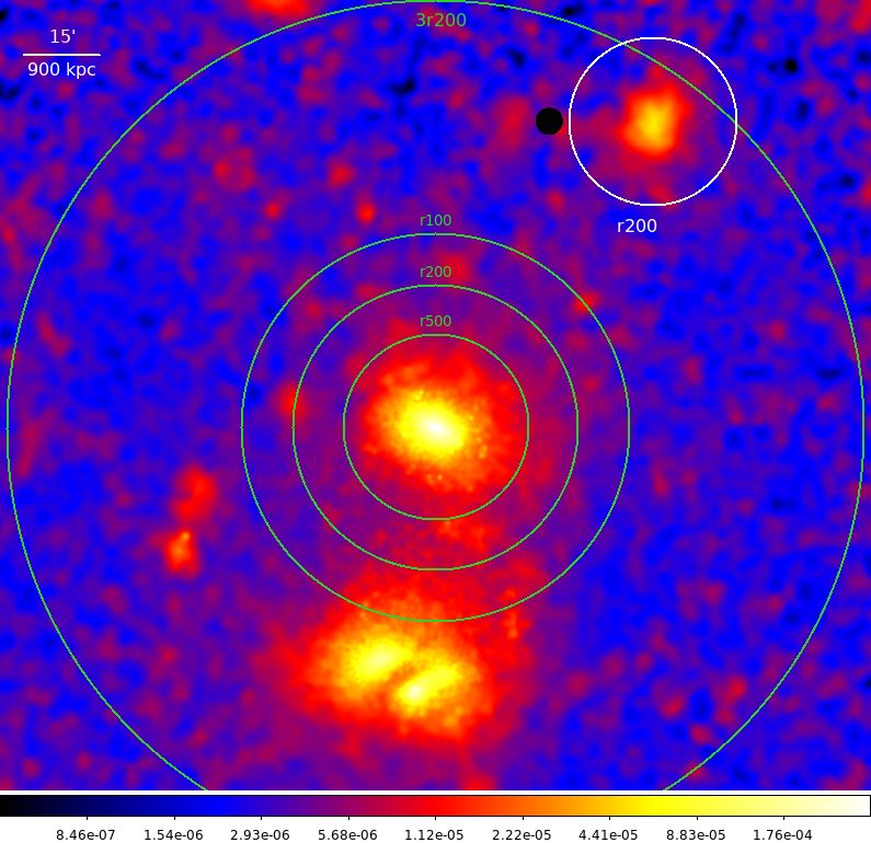
A&A proofs: manuscript no. main_NorthernClump

Fig. 1: eROSITA Particle-Induced Background (PIB) subtracted, exposure corrected, absorption corrected image in the energy band 0.5 − 2.0 keV,
zoomed-in to A3391 and the Northern Clump region. The image has been adaptively-smoothed with SNR set to 15. The point sources have been
removed and refilled with their surrounding background values. The green circles depict some characteristic radii of A3391, while the white circle
depicts the R200 of the Northern Clump.

2010), as well as where the Warm-Hot Intergalactic Medium                 Böhringer 1999; Werner et al. 2008; Fujita et al. 2008), and also
(WHIM) can be found (Rost et al. 2020). The large-scale cos-              in the outskirts of galaxy clusters (e.g., Reiprich et al. 2013; Bul-
mological simulations of a standard ΛCDM model (Cen & Os-                 bul et al. 2016; Nicastro et al. 2018). The binary galaxy cluster
triker 1999; Davé et al. 2001) predict that about 30 − 40% of             system Abell 3391 and Abell 3395 (A3391/95) is amongst the
the total baryons in the Universe reside in the WHIM, and thus            best candidates to conduct this search.
it is believed that the WHIM might be a solution to the miss-                 The A3391/95 system has been observed by numerous in-
ing baryon problem. However, with electron densities falling be-          struments of different wavelengths. Earlier studies of the system
tween ne ≈ 10−6 − 10−4 cm−3 and temperatures in the range of              using ROSAT and ASCA (Tittley & Henriksen 2001) show that
T = 105 − 107 K (Nicastro et al. 2017), detecting the WHIM                the gas from the region between the northern cluster (A3391)
is rather difficult (Werner et al. 2008). Bond et al. (1996) pre-         and the double-peaked southern cluster (A3395S/N) is consistent
dicted that the presence of the filaments are expected to be the          with a filament. Meanwhile, more recent studies using XMM-
strongest between highly-clustered and aligned clusters of galax-         Newton, Chandra, and Suzaku show that the properties of the
ies. Based on this prediction, it is sensible to conduct the search       gas are more in agreement with tidally-stripped Intra-Cluster
for the WHIM between a pair of galaxy clusters (e.g., Kull &              Medium (ICM) gas originated from A3391 and A3395, indi-

Article number, page 2 of 24
Angie Veronica et al.: The eROSITA View of the Abell 3391/95 Field: The Northern Clump

cating an early phase of cluster merger (Sugawara et al. 2017;              and the infalling group from the Magneticum Simulation. In Sec-
Alvarez et al. 2018).                                                       tion 5, we summarize our findings and conclude the results.
    The A3391/95 system is also one of the Performance Veri-                     Unless stated otherwise, all uncertainties are at the 68.3%
fication (PV) targets of the newly-launched German X-ray tele-              confidence interval. The assumed cosmology in this work is a
scope on board the Spectrum-Roentgen-Gamma (SRG) mission,                   flat ΛCDM cosmology, where Ωm = 0.3, ΩΛ = 0.7, and H0 =
the extended ROentgen Survey with an Imaging Telescope Ar-                  70 km/s/Mpc. At the Northern Clump redshift z = 0.0511, 100
ray (eROSITA). With large Field-of-View (FoV) of ∼ 1 degree                 corresponds to 0.998 kpc.
in diameter, the scan-mode observation, and superior soft X-ray
effective area (the effective area of the combined seven eROSITA
Telescope Modules (TMs) is slightly higher than the one of                  2. Data Reduction and Analysis
XMM-Newton (MOS1+MOS2+pn) in the 0.5 − 2.0 keV energy                       We list all eROSITA, XMM-Newton, and Chandra observations
band) (Merloni et al. 2012; Predehl et al. 2021), eROSITA al-               used for imaging and spectral analysis in Table 1.
lows us to capture the A3391/95 system beyond R100 with a good
spectral resolution.
    In total, four eROSITA PV observations were performed                   2.1. eROSITA
on the A3391/95 system, including three raster scans and one
                                                                            The A3391/95 PV observations are listed in Table 1. In this work
pointed observation. Combining all the available observations
                                                                            we use eROSITA data processing of configuration c001. The data
an area of ∼ 15 deg2 are covered. This reveals a breathtaking
                                                                            reduction of all 16 eROSITA data sets are realized using the ex-
view of the A3391/95 system that has only been seen in simu-
                                                                            tended Science Analysis Software (eSASS, Brunner et al., sub-
lations before, such as the discovery of a long continuous fila-
                                                                            mitted) version eSASSusers_201009. The eROSITA data reduc-
ment (∼ 15 Mpc) from the projected north towards the south of
                                                                            tion and image correction steps are described in great detail in
the A3391/95 system. This indicates that the system is a part of
                                                                            Section 2.1 of Reiprich et al. (2021). The image correction in-
a large structure. eROSITA also found that the bridge gas con-
                                                                            cludes Particle-Induced Background (PIB) subtraction, exposure
sists of not only the hot gas, which further confirms the tidally-
                                                                            correction, and Galactic absorption correction across the FoV.
stripped originated gas scenario, but also of warm gas from a
filament (Reiprich et al. 2021). A detailed eROSITA study focus-
ing on the bridge will be discussed in Ota et al. (in prep.) Addi-          2.1.1. Imaging Analysis
tionally, some clumps that seem to fall into the system are also
discovered, two of which reside in the Northern and the Southern            The energy band for the imaging analysis is restricted to 0.5 −
Filaments, namely the Northern Clump1 (MCXC J0621.7-5242                    2 keV, with the lower energy limit used for the Telescope Mod-
cluster, Piffaretti et al. 2011 and also referred as MS 0620.6-5239         ules (TMs) with on-chip filter (TM1, 2, 3, 4, 6; the combination
cluster, Tittley & Henriksen 2001; De Grandi et al. 1999) and the           of these TMs is referred to as TM8) set to 0.5 keV, while for
Little Southern Clump, respectively (Reiprich et al. 2021).                 the the TMs without on-chip filter (TM5 and 7; the combina-
    After eROSITA’s discovery, follow-up observations were                  tion of these TMs is referred to as TM9) it is set to 0.8 keV
performed by XMM-Newton and Chandra on the Northern                         due to the optical light leak contamination (Predehl et al. 2021).
Clump. This biggest infalling clump in the A3391/95 field is a              The count rates of the final combined image correspond to an
galaxy cluster, located at redshift z = 0.0511 (Tritton 1972; Pif-          effective area given by one TM with on-chip filter in the energy
faretti et al. 2011). It hosts a Fanaroff-Riley type I (FRI) radio          band 0.5 − 2 keV. The final PIB subtracted, exposure corrected,
source, PKS 0620-52 (Trussoni et al. 1999; Venturi et al. 2000).            and Galactic absorption corrected image is shown in Figure 1.
This source is associated with the cluster’s Brightest Cluster              The image has been adaptively-smoothed to enhance low sur-
Galaxy (BCG), 2MASX J06214330–5241333 (Brüggen et al.                       face brightness emission and large scale features, with Signal-
2021). This source is featured with a pair of asymmetric Wide-              to-Noise Ratio (SNR) is set to 15. We note that the Northern
Angle-Tails (WAT) radio lobes (Morganti et al. 1993; Trussoni               Clump appears boxy, which could be the result of ram-pressure
et al. 1999; Venturi et al. 2000), with the north-east lobe extend-         stripping as it interacts with the atmosphere of the A3391 cluster
ing up to 40 (240 kpc), while the north-western lobe up to 2.50             or the filament, or both. In this work, we will focus on study-
(150 kpc) (Brüggen et al. 2021).                                            ing the properties of the Northern Clump out to its R200 , while
    In this work, we investigate the morphology, thermal, and               a more detailed study about the filaments observed by eROSITA
chemical properties of the Northern Clump utilizing all avail-              around the A3391/95 system will be carried out by Veronica et
able eROSITA, XMM-Newton, and Chandra observations of the                   al. (in prep).
cluster. The cluster core is probed further with the help of the                 Thanks to the large eROSITA FoV and the SRG scan mode,
ASKAP/EMU radio data (Norris et al. 2011), Planck-y map,                    in which most of the observations were taken, the CXB could
and DECam optical data. Furthermore, we identify an infalling               be modelled from an annulus with an inner and outer radius of
galaxy group, resembling the observed Northern Clump, in the                250 and 350 , respectively. The annulus is centered at the X-ray
analog A3391/95 system from the Magneticum Simulation (Biffi                emission peak of the cluster determined by Chandra at (α, δ) =
et al. 2021, subm.) and discuss its properties in comparison to             (6 : 21 : 43.344, −52 : 41 : 33.0). Since the CXB region is at
observations to support their interpretation.                               1.5 − 2.1R200 2 , it ensures minimum cluster emission in the CXB
    This paper is organized as follows: in Section 2, we describe           region. This region also stays beyond R100 of A3391. Within the
the observations, data reduction, and the analysis strategy. In             13.50 radius, we utilize the XMM-Newton point source catalogue
Section 3, we present and discuss the analysis results. In Section          and beyond this radius we use eROSITA detected point source
4, we provide some insights about the analog A3391/95 system                catalogue, which was generated following the same procedure as
                                                                            2
1
   As the extended objects detected in the A3391/95 field are called           All the cluster radii in this work are calculated using the relations
"clumps", we refer this specific galaxy cluster found in the north of the   stated in Reiprich et al. (2013), e.g., r500 ≈ 0.65r200 , r100 ≈ 1.36r200 , and
main system as the Northern Clump                                           r2500 ≈ 0.28r200 .

                                                                                                                           Article number, page 3 of 24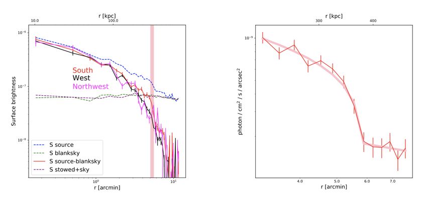
A&A proofs: manuscript no. main_NorthernClump

                                        Table 1: All observations of the Northern Clump used in this work.

        Observing Date               ObsID           Exposure∗ [ks]    R.A. (J2000)                                     Dec. (J2000)
                                                                 eROSITA
            October 2019         300005 (scan)             55         06h 26m 49.44s                                -54d 040 19.2000
            October 2019         300006 (scan)             54         06h 26m 49.44s                                -54d 040 19.2000
            October 2019         300016 (scan)             58         06h 26m 49.44s                                -54d 040 19.2000
            October 2019        300014 (pointed)           35         06h 26m 49.44s                                -54d 040 19.2000
                                                               XMM-Newton
             March 2020           0852980601           73, 77, 65     06h 21m 42.55s                                -52d 410 47.400
                                                                  Chandra
            October 2010              11499                20         06h 21m 43.30s                                -52d 410 33.300
             April 2020               22723                30         06h 21m 25.05s                                -52d 430 09.900
             May 2020                 22724                30         06h 21m 42.53s                                -52d 450 24.700
             April 2020               22725                30         06h 21m 22.30s                                -52d 420 10.700
        ∗
            The exposure times listed for eROSITA are the average filtered exposure time across the available TMs of each observation.
            The listed XMM-Newton exposure times are the values after the SPF filtering for MOS1, MOS2, and pn cameras, respectively.
            The exposure times listed for Chandra are also the filtered exposure time.

XMM-Newton (see Section 2.2). The point sources are excluded
both in imaging and spectral analyses.                                                                    0.1
                                                                           normalized counts s−1 keV−1

                                                                                                         0.01
2.1.2. Spectral Analysis
All eROSITA spectra, the Ancillary Response Files (ARFs), and                                            10−3

the Response Matrix Files (RMFs) for the source and back-
ground region are extracted using the eSASS task srctool. Un-                                            10−4

less stated otherwise, the spectral fitting for all eROSITA spectra
is performed with XSPEC (Arnaud 1996) version: 12.10.1.                                                  10−5

    The third eROSITA scan observation (ObsID: 300016),
                                                                           (data−model)/error

                                                                                                           2
where all seven eROSITA TMs are available, is employed for the
spectral analysis of the Northern Clump. Due to the contamina-                                             0
tion by the nearby bright star, Canopus, some portions of the data
are rejected from the analysis (see Reiprich et al. 2021), which                                          −2

further reduces the number of photons for the Northern Clump.                                                   1   2
                                                                                                                         Energy (keV)
                                                                                                                                        5

To ensure enough photon counts, the only eROSITA spectral fit-                                                                               averonica 26−May−2021 21:25

ting done for the Northern Clump in this work is to constrain             Fig. 2: eROSITA spectrum of the Northern Clump from an annulus of
the kB T 500 from an annulus with inner and outer radii of 2.40           2.4 − 60 , fitted in the energy range 0.7 − 9.0 keV. The spectra and the
and 60 (corresponding to 0.2 − 0.5R500 , see Subsection 2.2.2).           corresponding response files of TM3 and TM4 are merged for a better
The same definition of CXB region as in the imaging analysis              visualization. The black points are the Northern Clump spectral data,
is used. We follow the X-ray spectral fitting procedure described         while the black, red, green, and blue lines represent the total model, the
in Ghirardini et al. (2021) and Liu et al. (submitted) with some          cluster model, the instrumental background model, and the CXB model,
modifications for consistency with the XMM-Newton and Chan-               respectively.
dra spectral fitting.
    The total eROSITA model includes the absorbed thermal
emission for the cluster, which is modelled using phabs×apec,             2.2. XMM-Newton
two absorbed thermal models for the Milky Way Halo (MWH)                  The data reduction steps of the XMM-Newton data sets of the
and Local Group (LG), an unabsorbed thermal model for the                 Northern Clump observation are realized using HEASoft version
Local Hot Bubble (LHB), and an absorbed power-law for the                 6.25 and the Science Analysis Software (SAS) version 18.0.0
unresolved AGN. The parameters of the eROSITA CXB compo-                  (xmmsas_20190531_1155).
nents are listed in Table 2. The instrumental background is mod-              For all XMM-Newton instruments, we filtered out the time in-
elled based on the results of the eROSITA Filter Wheel Closed             tervals contaminated by Soft Proton Flares (SPF) (e.g., De Luca
(FWC) data analysis. The normalizations of the instrumental               & Molendi 2004; Kuntz & Snowden 2008; Snowden et al. 2008).
background components are thawed during the fit. The fitting is           The procedure started by constructing the light curve in the en-
restricted to the 0.7 − 9.0 keV band, with the lower energy limit         ergy band 0.3 − 10.0 keV from the entire FoV. The mean value of
set to 0.8 keV for TM5 and TM7 and to 0.7 keV for the other               the counts is estimated by fitting a Poisson law to the counts his-
TMs. Source and CXB spectra for the individual TMs are fitted             togram. Then a ±3σ clipping is applied, such that any time inter-
simultaneously. An example of eROSITA spectrum and its fitted             vals above and below the 3σ threshold are considered contam-
model is shown in Figure 2.                                               inated by the SPF and rejected from further steps. Lightcurves
    The solar abundance table from Asplund et al. (2009) is               from each of XMM-Newton’s detectors are shown in Appendix
adopted and the C-statistic (Cash 1979) is implemented.                   A. To check whether there is still any persisting soft proton back-
                                                                          ground in our data, we calculated the ratio of count rates within

Article number, page 4 of 24
Angie Veronica et al.: The eROSITA View of the Abell 3391/95 Field: The Northern Clump
Table 2: Information of the parameters and their starting fitting values Another contamination when studying the ICM gas might
of the eROSITA CXB components. come from the point sources that are distributed across the FoV.
Therefore, it is required to detect and excise the point sources,
component parameter value comment for example in the calculation of surface brightness profiles and
phabs NH† 0.04 fix spectral analysis. To detect the point sources in the observation,
apec (LHB) kB T [keV] 0.099 fix we implement the procedure described in Pacaud et al. (2006)
Z [Z ] 1 fix and Ramos-Ceja et al. (2019). Firstly, wavelet filtering is ap-
z 0 fix plied on the combined detector image in the soft energy band
norm∗ 1.0 × 10⁻⁸ vary (0.5 − 2.0 keV). Afterwards, an automatic detection of point
apec (MWH) kB T [keV] 0.225 fix sources and catalogue generation are performed on the wavelet-
Z [Z ] 1 fix filtered image by the Source Extractor software (SExtractor,
z 0 fix Bertin & Arnouts 1996). Lastly, we carry out a manual inspec-
norm∗ 1.0 × 10⁻⁸ vary tion on the soft and hard energy band images (2.0 − 10.0 keV)
apec (LG) kB T [keV] 0.5 vary to list any point sources that may be missed by the automatic
Z [Z ] 1 fix detection. To generate a surface brightness image, the areas
z 0 fix where the point sources are removed are refilled with random
norm∗ 1.0 × 10⁻⁸ vary background photons, i.e., the ghosting procedure. The ghosted-
pow Γ 1.4 fix surface brightness images are used only for visual inspection.
(unresolved AGN) norm∗∗ 3.4 × 10⁻⁷ vary
†
[1022 atoms cm−2 ] 2.2.1. Imaging Analysis
∗
[cm−5 /arcmin2 ]
∗∗
[photons/keV/cm2 /s/arcmin2 at 1 keV]
the FoV (IN) to those of the unexposed region of the MOS detec-
tors (OUT) (De Luca & Molendi 2004). The obtained IN/OUT
ratios for each detector are around unity, which implies the re-
tained data are not contaminated by soft protons. After this SPF
filtering, we are left with ∼ 73 ks, ∼ 77 ks, and ∼ 65 ks for MOS1,
MOS2, and pn, respectively.
We checked for “anomalous state” in the detectors’ chips.
This is usually indicated by a low hardness ratio and high total
background rate (Kuntz & Snowden 2008). Since, in such cases,
there is not yet a robust method to model the spectral distribution
of the low energy background, any CCD affected by this anoma-
lous state was rejected in further analysis. This resulted in the
conservative exclusion of MOS1-CCD4 and MOS2-CCD5. In
addition, MOS1-CCD6 and MOS1-CCD3 were not operational
during this observation, due to the previous micro-meteoride im-
pacts (ESA: XMM-Newton SOC 2020).
Utilizing the FWC data, the Quiescent Particle Background
(QPB) (Kuntz & Snowden 2008) is modelled and then sub-
tracted from the observation. We follow the procedure described
in Ramos-Ceja et al. (2019). First, the cleaned observation data
is matched with the suitable FWC data and then this FWC tem-
plate is re-projected to the sky position. Afterwards, rescaling
factors are calculated to renormalize the QPB template to a level Fig. 3: XMM-Newton count rate image of the Northern Clump in the
comparable with that of the observation. This renormalization is energy band 0.5 − 2.0 keV, overlaid with the ASKAP/EMU radio con-
calculated separately for each MOS CCD and pn quadrant based tour (black). The anomalous CCD chips are removed and the QPB is
on their individual count-rates in unexposed regions. The renor- subtracted from the image. The sectors are South (S), West (W), North-
malization of the central MOS CCD chips that do not have any West (NW), North (N), North-East (NE), and East (E). The white circle
and cyan square depict the outermost annuli of corresponding setups.
unexposed regions relies on the unexposed regions of the best The radius of the circle is 100 and the half-width of the square is 7.50 .
correlated surrounding CCD chips as determined by (Kuntz & Gaussian smoothing with kernel radius of 7 pixels is applied to the im-
Snowden 2008). For spectroscopic analysis, global renormaliza- age.
tion factors are calculated in the energy bands 2.5 − 5.0 keV and
8.0−9.0 keV for MOS cameras, and 2.5−5.0 keV for pn camera. We construct XMM-Newton’s X-ray surface brightness (S X )
This energy selection aims to include the bands were the instru- profiles using the combined photon image and exposure map
mental background would have the most impact on the spectral from the XMM-Newton detectors (MOS1, MOS2, and pn) in the
analysis, while avoiding the Fluorescence X-ray (FX) emission energy band 0.5 − 2.0 keV. Since the ghosting procedure used to
lines present for the EPIC cameras. For imaging analysis, on the generate surface brightness images does not represent the exact
other hand, the template renormalization process relies on the true counts from the ICM gas, we preferred to mask these point
exact same band that is used for the science analysis. source regions in the calculation of the S X profile. The first S X
profile is calculated from 60 concentric annuli placed around the
Article number, page 5 of 24A&A proofs: manuscript no. main_NorthernClump
Chandra X-ray emission peak at (α, δ) = (6 : 21 : 43.344, −52 : term, phabs×apec3 , represents the absorbed cluster emission
41 : 33.0). With 1000 increments between each annulus, the whole from the source region. The temperature kB T , metallicity Z, and
arrangement covers radial distance of 100 from the center. While normalization norm of this cluster emission component are left
the QPB was subtracted from the data, the CXB was estimated to vary and linked across the detectors.
from an annulus with an inner radius of 120 and an outer radius The apec’s parameter norm is defined as
of 13.250 , respectively. Then, the estimated S X from this back-
ground region was subtracted from the source regions.
10−14
Z
A second S X profile is also constructed. The setup consists norm = ne nH dV, (3)
of 45 concentric box-shaped “annuli” centered at the same peak 4π[DA (1 + z)]2
coordinates. Between each annulus there is a 2000 width incre-
where DA is the angular diameter distance to the source in the
ment. This implies that the width of each box-shaped annulus
unit of cm, while ne and nH are the electron and hydrogen densi-
corresponds to the diameter of each circular annulus. The half-
ties in the unit of cm−3 , respectively.
width of the outermost box annulus is 7.50 . The setup is angled at
173◦ , which is chosen visually to follow the shape of the North-
Table 3: Information of the parameters and their starting fitting values
ern Clump. The same X-ray background region as in the circular of the XMM-Newton CXB components.
annuli setup is used. To investigate, whether the boxiness could
be an artefact originating from the MOS detectors’ central chips,
component parameter value comment
a S X profile from pn-only data and using the box annuli setup is
calculated as well. phabs NH† 0.046 fix
We fitted each of the setups with a single β-model (Cavaliere apec1 (LHB) kB T [keV] 0.099 fix
& Fusco-Femiano 1976), which is written as Z [Z ] 1 fix
z 0 fix
!−3β+ 12 norm∗ 1.7 × 10⁻⁶ vary
R2 apec2 (MWH) kB T [keV] 0.225 fix
S X (R) = S X (0) 1 + , (1) Z [Z ] 1 fix
rc2
z 0 fix
where R is the projected distance from the center, S X (0) is the norm∗ 7.3 × 10⁻⁷ vary
normalization factor, rc is the estimated core radius, and β is the pow Γ 1.4 fix
surface brightness slope. (unresolved AGN) norm∗∗ 5 × 10⁻⁷ vary
To better address the features in any particular direction, the †
[1022 atoms cm−2 ]
S X profiles in the projected south, west, northwest, north, north- ∗
[cm−5 /arcmin2 ]
east, and east directions are constructed, as well. For these sec- ∗∗
[photons/keV/cm2 /s/arcmin2 at 1 keV]
torized S X profiles, all XMM-Newton detectors are employed in
both circular and box annuli setups. The configuration of the sec-
tors is displayed in Figure 3. To ensure a cluster-emission-free background region, the
ROSAT All-Sky Survey (RASS) data are utilized to constrain all
of the sky background components, in particular the MWH as
2.2.2. Spectral Analysis well as CXB normalization. The RASS data are extracted using
Unless stated otherwise, the spectral fitting for all XMM-Newton the X-ray background tool3 . The specified background region
spectra is performed with XSPEC (Arnaud 1996) version: 12.10.1 is an annulus centered at the Chandra center, with an inner ra-
using the following model, dius of 0.58◦ and an outer radius of 0.9◦ . To avoid having cluster
emission from A3391, we manually removed some of the RASS
ModelXMM = constant × (apec1 + phabs × (apec2 + background region that is within R100 of the A3391 cluster. This
powerlaw) + gauss1 + gauss2 + gauss3 + reduces the number of detected pixels from 38 to 34.
The variety of overlap area between each annulus and each
gauss4 + gauss5 ) + phabs × apec3 , (2) individual camera/CCD combination can result in some very low
SNR spectra being extracted, for which a background model can
where the first term consists of the CXB and XMM-Newton’s not always be robustly constrained. For this reason, we opted to
known instrumental lines, scaled to the areas of the source re- combine the spectra of all CCDs for a given annulus, and sta-
gions (constant, specified in units of arcmin2 ). phabs is the tistically subtract the rescaled FWC spectrum rather than mod-
absorption parametrized by the hydrogen column density, NH , elling their spectra. The co-addition of rescaled spectra for the
along the line of sight. The NH values used in this work are different CCDs implies that our background spectra no longer
taken from the A3391/95 total NH map described in Section 2.5 follow Poisson statistics and therefore we use the χ2 -statistic
of Reiprich et al. (2021). apec1 is the X-ray emission model to for parameter estimation, after ensuring that each bin contains
account for the LHB, while apec2 is for the MWH. powerlaw enough photons (>25). Additionally, since we use the RASS
is the power-law component for the unresolved AGN. The in- background, which is Gaussian data, to estimate the CXB nor-
formation regarding the CXB components and their starting fit- malizations, the choice is believed to be sensible. However, we
ting parameter values are listed in Table 3. Since the Fluores- also performed several tests using pgstat statistic from XSPEC,
cent X-ray (FX) emission lines of the XMM-Newton cameras where the source data is treated as Poisson data (C-statistic)
are not convoluted in the Auxiliary Response Files (ARF), we and the background as Gaussian. The resulting cluster param-
modelled the lines with the other background components as the eters of these tests are always consistent within the 1σ error bars
gaussi ’s. The modelled FX lines include the Al-Kα at 1.48 keV of the χ2 -statistic fitting results. Hence, the choice of the used
(for MOS and pn cameras), Si-Kα at 1.74 keV (MOS cameras), statistics for XMM-Newton spectral fitting would not change any
Ni-Kα at 7.47 keV (pn camera), Cu-Kα at 8.04 keV (pn camera),
3
and Zn-Kα at 8.63 keV (pn camera), respectively. The second HEASARC: X-Ray Background Tool
Article number, page 6 of 24Angie Veronica et al.: The eROSITA View of the Abell 3391/95 Field: The Northern Clump
N
E
400 kpc
Fig. 4: Left: Mosaic Chandra ACIS-I image of the northern clump. The image is blanksky background subtracted, exposure corrected, and point-
source refilled. Right: The mosaic exposure map corresponding to the left image. Red, black, and magenta pie regions represent the regions used
to derive the surface brightness profiles of the south, west, and northwest directions as shown in Fig 8.
main conclusions. We present the results of the pgstat tests in ting to take into account the emission originated from the AGN
Appendix D, Figure D.1. To minimize the effect of the detector of the BCG. Three different fitting methods are implemented for
noise in the lower energy, photons with E < 0.7 keV are ignored. this particular bin:
The solar abundance table from Asplund et al. (2009) is adopted.
1. The first method is to mask the AGN with a circle of 1500
We determined the kB T 500 in order to calculate the M500 , con-
radius. This is the method that is implemented to the central
sequently the R500 . kB T 500 is calculated through an iterative pro-
bin during the simultaneous fitting described above.
cedure, such that we extract and fit spectra from an annulus cen- 2. The second method involves constraining the AGN photon
tered at the Chandra center, varying the inner and outer radii index and normalization from Chandra observation. Here,
until they correspond roughly to the 0.2 − 0.5R500 cluster region. the masking is lifted out. Since XMM-Newton and Chan-
Based on this, we obtained kB T 500 = 1.99 ± 0.04 keV from an dra observations of the Northern Clump are performed al-
annulus with inner and outer radii of 2.40 and 6.00 , respectively. most simultaneously, little to no temporal variation from the
We input this value into the mass-temperature (M − T ) scaling AGN can be expected (e.g., Maughan & Reiprich 2019). The
relation by Lovisari et al. (2015), method and the resulting AGN parameter values from the
spectral fitting are discussed in Subsection 2.3.3. We freeze
log(M/C1) = a · log(T/C2) + b, (4) Chandra’s parameter values during the XMM-Newton spec-
tral fitting of the first bin.
where a = 1.65 ± 0.07, b = 0.19 ± 0.02, C1 = 5 × 10¹³ h−1 70 M ,
3. Lastly, to account for the expected multi-temperature struc-
and C2 = 2.0 keV. Assuming spherical symmetry and taking 500 ture in this region, we performed a two-temperature struc-
times the critical density of the Universe at the Northern Clump ture fitting in addition to the AGN component. Due to the
redshift as ρ500 (z = 0.0511) = 4.82 × 10⁻²⁷ g cm−3 , we obtain statistics, the normalization and the metallicity of the multi-
M500 = (7.68 ± 0.43) × 1013 M and R500 = (10.62 ± 0.20)0 ≈ temperature components are linked, while the second tem-
(636.03 ± 12.03) kpc. These values are 19% and 7% lower than perature are set to be half of the first.
the reported values in Piffaretti et al. (2011) (M500 = 9.47 ×
1013 M and R500 = 682 kpc), which were determined using the 2.3. Chandra
L − M relation, instead.
We also analyze the spectra in three different directions of the We analyzed a total of 110 ks Chandra observations on the
cluster, such as the south, west, and north with Position Angle Northern Clump as listed in Table 1, including three ACIS-
(P.A.) from 250◦ to 305◦ , 20◦ to 305◦ , and 70◦ to 100◦ , respec- I observations taken in 2020 and one ACIS-S observation in
tively. At larger radii, i.e., 4 − 12.50 , due to the removed MOS1- 2010. CIAO 4.12 and CALDB 4.9.3 are used for the Chandra
CCD chips we use pn-only spectra in the north, and MOS2+pn data reduction. All the observations are reprocessed from level
spectra in the south and west. 1 events using the CIAO tool chandra_repro to guarantee the
We always keep the first bin as a full annulus, instead of a latest and consistent calibrations. Readout artifacts from the cen-
sector in any specific directions. We conduct a more detailed fit- tral bright AGN are removed from the reprocessed events using
Article number, page 7 of 24A&A proofs: manuscript no. main_NorthernClump
acisreadcorr. We filtered background flares beyond 3σ using dex of 2.5±0.07 and a best-fit luminosity of 5.7±0.3×1041 erg/s
the light curve filtering script lc_clean; clean exposure times in the 2.0 − 10.0 keV when using the observation taken in 2020,
are listed in Table 1. We combine all the observations to resolve which is used for the AGN modelling in the XMM-Newton anal-
faint point sources. The Chandra PSF varies significantly across ysis.
the FoV. For each observation, we produce a PSF map for an
energy of 2.3 keV and an enclosed count fraction of 0.393. We
2.4. ASKAP/EMU, DECam, and Planck Data
obtain an exposure-time weighted average PSF map from these
four observations. Point sources are detected in a 0.3 − 7.0 keV We use the ASKAP/EMU radio image and DECam images, as
mosaic image with wavdetect, supplied with this exposure- well as the Planck y-map for overlays generated as described in
time weighted PSF map. The detection threshold was set to 10−6 . detail in Reiprich et al. (2021).
The scales ranged from 1 to 8 pixels, increasing in steps of a fac-
tor of 2. We adopt the blank sky background for the imaging and
spectral analyses. A compatible blank sky background file was 3. Results
customized to each of the event file using the blanksky script.
3.1. Boxiness, Tail, and X-ray Cavity in Images
As shown in Subsection 3.2, the surface brightness of our blank
sky background is consistent with the sum of the stowed back-
ground and the astrophysical background.
2.3.1. Imaging Analysis
We only include the three ACIS-I observations taken in 2020
for the imaging analysis due to the different backgrounds, re-
sponses, FoVs, and calibrations between these observations and
the ACIS-S observation taken in 2010. All the observations
are reprojected to a common tangent point using reproject_obs.
Images in the 0.5 − 2.0 keV energy band and their expo-
sure maps are produced using flux_obs. Point sources iden-
tified by wavdetect are replaced with the surface brightness
from the immediate surrounding regions using dmfilth. Scaled
blanksky images are produced using blanksky_image. A final
background-subtracted and exposure corrected mosaic image of
the Northern Clump is shown in Figure 4.
2.3.2. Spectral Analysis
We include all four existing Chandra observations for the spec-
tral analysis. Spectra are extracted using specextract from
point-source excised event files for regions of consecutive sec-
tional annuli in the south and west directions, ranging from
δr = 0.50 at the cluster center to δr = 1.670 at r = 6.680 . The cor-
responding response files and matrices were produced for each
spectrum using specextract. Blanksky background normal-
ized to the count rate in the 9.5 − 12.0 keV energy band of each Fig. 5: XMM-Newton surface brightness images (left) and
observation was applied. All the spectra were grouped to have at adaptively-smoothed images (right) in the energy band 0.5 − 2
least one count per energy bin and restricted to the 0.7 − 7.0 keV keV. The SNR of the adaptively-smoothed images is set to 15.
range. The spectral fitting was performed with PyXspec 2.0.3. Top: MOS1+2+pn combined. Bottom: pn-only.
Our spectral model takes the form of phabs×apec, representing
a foreground-absorbed thermal component. The total NH value As observed in the clean images shown in Figure B.1, the
of 4 × 1020 cm−2 is taken from the A3391/95 total NH map de- main body of the Northern Clump is well-embedded in the cen-
scribed in Reiprich et al. (2021). C-statistics (Cash 1979) is used tral chips of MOS1 (top left) and MOS2 (top right) cameras. A
for parameter estimation. The solar abundance table of Asplund question arises, whether the boxyness of the system is intrinsic to
et al. (2009) is adopted. Due to low photon counts, we find it the cluster itself, or rather an artefact caused by the central MOS
necessary to fix the metallicity at 0.3Z . chips. The boxy shape of the cluster can still be recognized in the
pn image (bottom left), although not as prominent. To further in-
vestigate this question, we generate exposure corrected images,
2.3.3. Central AGN
as well as adaptively-smoothed images using MOS1+2+pn data
We characterize the property of the central AGN detected at and pn-only data, where the latter should not be affected by the
equatorial coordinates of (α, δ) = (6 : 21 : 43.304, −52 : 41 : CCD chips placement. The adaptive smoothing procedure is re-
33.153). Spectra of the central r = 200 were extracted from clean alized using the SAS task, asmooth, smoothstyle=‘adaptive’.
events files with point sources included. Spectra from the sur- We set the SNR of the adaptive smoothing to 15. Through adap-
rounding r = 2−500 were used as the local background. We fit the tive smoothing we also aim to enhance any soft emission, espe-
spectrum to a simple absorbed power-law model and fixed the cially in the cluster outskirts. The resulting images are displayed
column density NH = 4×1020 cm−2 . We obtain a steep photon in- in Figure 5. We observe similarity in the morphology of the clus-
Article number, page 8 of 24Angie Veronica et al.: The eROSITA View of the Abell 3391/95 Field: The Northern Clump
100 kpc
4.61e-08 2.84e-08 1.03e-07 1.78e-07 2.53e-07 3.27e-0
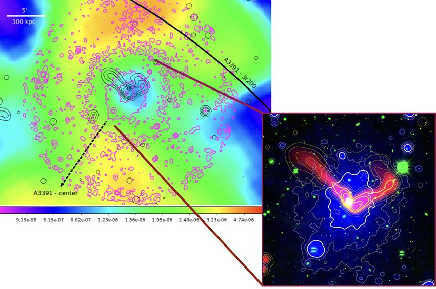
Fig. 6: Left: Chandra unsharp masked image of the central region of the Northern Clump. Right: XMM-Newton residual image. The northern
yellow arrow shows the 5.30 projected length of the tail emission. The enhancement in the south is indicated by the southern yellow arrow and
the center of A3391 cluster is pointed by the dashed-line white arrow. Gaussian smoothing with kernel radius of 3 pixels is applied to the image.
Black and white contours in both images represent the ASKAP/EMU radio continuum emission.
ter in the two types of images, i.e., the boxy shape and indication r ≈ 2.090 (125 kpc) to the east and west of the cluster center.
of tail-like emission projected northward. We further overlay the ASKAP/EMU radio continuum emission
We present a composite X-ray+radio+optical image in Fig- of the cluster center. A seeming picture of X-ray cavities filled
ure 12 (left), focusing on the central region of the Northern with radio lobes starts to emerge, as observed for other clusters
Clump. We utilize the XMM-Newton count rate image in soft (e.g., Bîrzan et al. 2004; McNamara & Nulsen 2007).
band (blue color and white contour), the ASKAP/EMU radio From the presented XMM-Newton and Chandra images, and
image (red color and yellow contour), and DECam Sloan g- with the help from ASKAP/EMU radio image, as well as the
band image (green). The denser X-ray emission of the North- DECam optical image, we identify clear indications of Northern
ern Clump shows an asymmetrical morphology and has a sharp Clump’s boxyness, tail-like emission in the north, and hint of
edge pointing at the projected southwest direction – towards the X-ray cavities that coincide with the radio lobes.
A3391 center. We notice that the opening angle of the WAT ra-
dio source indicates movement towards the south. While looking
3.2. X-ray Surface Brightness (S X ) Profiles
at the bent direction of both radio lobes towards the northeast,
the central radio source seems to move towards the southwest. 3.2.1. XMM-Newton
We speculate that the radio lobes might have ”escaped” from
hot gas confinement and the change in direction is due to mo- The full azimuthal S X profiles of the three different setups can
tion through a lower density medium, as indicated by the con- be found in Appendix C. In all three profiles we observe a steep
tours. The central radio source may be moving locally within drop at around 50 < r < 60 (299.4 kpc < r < 359.28 kpc). More-
the Northern Clump towards the southwest as a result of, e.g., over, the overall shapes and residuals seen in the S X profiles of
sloshing, while globally, the Northern Clump moves towards the the box annuli setups using all XMM-Newton detectors and pn-
southeast. only data support the case that the boxy appearance of the clus-
We use unsharp masks in the Chandra image to highlight ter is not an artefact caused by the placement of the central MOS
substructures in the ICM. The original image was smoothed us- chip.
ing two different scales and one smoothed image was subtracted We present the sectorized S X profiles (using the box annuli
from the other to make the edges more visually appealing. This setup) in Figure 7 (right, top plot). The bottom plot of the Figure
technique can be mathematically expressed as shows the relative differences with respect to the corresponding
S X of the full azimuthal setups, which is to examine any excess
Û = I ∗ g − I ∗ h (5) or deficit of the surface brightness. The 1σ confidence region
where I stands for the original image and g and h are the two of the full azimuthal S X is plotted in grey. Hereafter, the full
smoothing scales, for which we chose g = 30 and h = 100 azimuthal S X profile will be referred to as the average S X profile.
pixels. As shown in Figure 6 (left), the unsharp masked im- The sectorized S X profiles using the circular annuli setup can be
age reveals regions with possible deficient surface brightness found in Appendix C.
Article number, page 9 of 24A&A proofs: manuscript no. main_NorthernClump
101
r [kpc]
102 103
r [kpc]
101 102
r2500
r2500
r500
r500
r200
10 2
10 13
SB [counts/s/arcmin2]
SB [ergs/s/cm2/arcmin2]
10 3
10 14
0.5 2.0 keV
CXB
QPB
1 box annuli
South
West
10 15
North-West
10 4
North
North-East
East
0.5 2.0 keV 1 box annuli
CXB-XMM
CXB-eRO 0.5
difference
XMM CXB region in eROSITA
relative
Chandra 0.0
10 16
XMM-Newton
XMM-Newton, corrected 0.5
eROSITA
10 1 100 101 1.0
r [arcmin] 100 101
r [arcmin]
Fig. 7: Left: Instrument independent, absorption corrected, and background subtracted S X profiles of Chandra (green), XMM-
Newton (blue), and eROSITA (red) in the energy band 0.5 − 2.0 keV. The blue, red, and black horizontal dashed lines are the CXB
levels of XMM-Newton, eROSITA, and eROSITA with XMM-Newton defined CXB region, respectively. Black points are the CXB
corrected XMM-Newton S X . The various radii are plotted in brown. Right: XMM-Newton S X profiles in the different directions of the
Northern Clump using the box annuli setup (top) and the relative differences with respect to the average surface brightness (bottom).
The grey shaded areas in both plots are the 1σ confidence region of the average S X . The various radii are plotted in brown. The
CXB and QPB level are plotted in orange and cyan dashed lines.
Some noticeable features among the different directions are ness depression at around r ≈ 2.050 (122.75 kpc) to the north-
present, such as the S X depression in the northeast, excess of the east and northwest of the center are observed. They coincide
S X in the south, and the enhancement towards the north. These with the lobes of the WAT radio source and also in agreement
features are seen in both setups, but they are more pronounced with what is found in Chandra unsharp masked image (Figure
in the box annuli setup. 6, left). In the south, a density enhancement relative to other
The depression in the northeast is at 10 < r < 30 (59.88 kpc < directions is revealed at predominantly around 20 < r < 50
r < 179.64 kpc). The S X gets closer to the average at around 40 (119.76 kpc < r < 229.40 kpc). Furthermore, we detect a clear
(239.52 kpc) and drops rapidly beyond this point. The largest tail of emission north of the Northern Clump, ∼ 70 (419.16 kpc)
fractional decrement in this direction, of 42%, occurs at 1.670 away from the center. This tail has a projected length of ∼ 5.30
(100 kpc). (317.4 kpc), as indicated by the northern yellow arrow in Figure
In the southern sector, S X enhancement is observed at around 6 (right).
20 < r < 60 (119.76 kpc < r < 359.28 kpc). The peak is at 4.170
(249.70 kpc) with a 67% enhancement. We suggest that the ori-
3.2.2. Chandra
gin of the surface brightness excess in this specific direction is
either from compressed gas caused by ram pressure or an ac- We derive the X-ray surface brightness profiles in south, west,
creted clump of cold gas from the Northern Filament, where the and northwest directions, ranging from the cluster center to radii
cluster resides. In both scenarios, the Northern Clump should be of 11.700 (700 kpc) as shown in Figure 8. We note a region of
falling towards the A3391 cluster along with the filament and enhanced brightness at around r = 5.840 (350 kpc) in the south
within the region where its mean density dominates, collapses direction relative to other directions. We fit the profile to a broken
from the filament will continue onto the system. power law profile with a density jump projected along the line of
We observe significant enhancement at larger radii in the sight
north direction consistent with the observed tail feature in the Z
image. A relative difference of 126% occurs at 7.50 (449.1 kpc). S (r) = norm F(ω)2 dl, where ω2 = r2 + l2 . (6)
The features seen in the sectorized S X profiles are present
in the residual image (Figure 6, right). The residual image is F(ω) is the deprojected density profile:
the result of dividing the surface brightness image by the spher-
ically symmetric model. We overlaid the residual image with
the ASKAP/EMU radio contour (white contour). Surface bright- ω−α1 if ω < rbreak
F(ω) =
(7)
1
jump ω−α2 otherwise,
Article number, page 10 of 24Angie Veronica et al.: The eROSITA View of the Abell 3391/95 Field: The Northern Clump
Fig. 8: Left: Blanksky background subtracted surface brightness profiles of the south (red), west (west), and northwest (magenta) directions in units
of counts/s/arcsec2 as measured with Chandra. The level of the tailored blanksky background (green dashed) and that of the stowed background
plus the astrophysical background (purple dashed) for the south direction are consistent. The blue dashed line represents the total emission from
both the source and background of the south direction. The vertical pink line marks the position of a possible density jump in the south direction.
Right: surface brightness profile zoomed in around the surface brightness edge in the south direction in units of photon/s/cm2 /arcsec2 . We fit the
data with a broken powerlaw density model (pink) and obtain a best-fit density jump of 1.45.
where α1 , α2 , jump, and rbreak are free parameters. We ob- eROSITA, 7.55 × 10⁻¹² ergs/cm2 /counts for XMM-Newton, and
tain a best-fit density jump of 1.45 ± 0.32 at r = 5.74 ± 0.170 1.72 × 10⁻⁹ ergs/photons for Chandra.
(344 ± 10 kpc). As the ICM temperature appears to be uniform The annulus used to estimate the XMM-Newton CXB level
across the edge (Figure 9), we assume that the pressure disconti- (12.0 − 13.250 (1.13 − 1.24R500 ), shown with the horizontal blue
nuity equals the density jump and calculate the associated Mach line) may still contain some cluster emission. In order to cor-
number (Landau & Lifshitz 1959): rect for this, we calculated the surface brightness of this same
!γ/(γ−1) background region using eROSITA data (horizontal black dashed
p0 γ−1 lines) and estimated the excess cluster surface brightness as the
= 1+ M (8)
p1 2 difference between the two background estimate (horizontal red
dashed line). We added back this excess surface brightness to
for which we obtain M = 0.48+0.30 −0.34 . Given a sound speed of obtain corrected XMM-Newton data points (plotted in black).
802 km/s for a 2.5 keV ICM, the central region of the North- The CXB correction results in better agreement between XMM-
+239
ern Clump is moving towards south at a speed of 386−274 km/s Newton and eROSITA, especially in the 7.0 − 10.00 radial range.
relative to the motion of the gas in the southern direction. The CXB-subtracted surface brightness profile is nearly flat be-
yond the R500 and out to the R200 . This may imply that at this
3.2.3. eROSITA , XMM-Newton, and Chandra regime, there is still some emission either from the cluster or the
filament in which the Northern Clump resides, or both.
We present S X profiles of all the used X-ray instruments in the Through this exercise, we show the complementary nature of
energy band 0.5 − 2.0 keV in Figure 7 (left). the three instruments. For instance, Chandra (green points) with
To correct for the effective area of different instruments and the best on-axis spatial resolution can cover as far as 300 from
absorption, each of the three profiles has been multiplied by the center, XMM-Newton (blue and black points) covers the in-
a conversion factor. For eROSITA and XMM-Newton, this con- termediate radial range with good statistics, and eROSITA (red
version factor is calculated by taking the ratio of the unab- points) with its wide FoV and scan mode delivers the cluster
sorbed energy flux to the absorbed count-rates in the 0.5 − 2 surface brightness out to 1.1R200 . The discrepancies in the cen-
keV band. We supplied the best-fit cluster parameters in the ter can be well-explained by the PSF effect. Moreover, although
2.4 − 60 , the (kB T 500 ) region and the on-axis response files of masked, the bright point source in the cluster center is likely to
an on-chip TM and MOS camera. To account for possible tem- contribute some of its emission to the central bins of eROSITA
perature changes across the radial ranges, we computed the con- and XMM-Newton profiles. Other causes, such as point source
version factor for 3 keV and 1.5 keV cluster emission, as well. detection and different background treatment could also play a
The variation is found to be less than 3%. For Chandra, whose role in the observed differences among the profiles.
exposure maps already include a correction for the telescope ef-
fective area in addition to vignetting, the conversion factor is
simply the ratio of the unabsorbed energy flux to the absorbed
photon flux. The factor is 9.87 × 10⁻¹² ergs/cm2 /counts for
Article number, page 11 of 24A&A proofs: manuscript no. main_NorthernClump
0 100 200
r [kpc] 300 400 500 0 100 200
r [kpc] 300 400 500
(0.7 - 7.0) keV (0.7 - 7.0) keV
XMM, South XMM, West
norm/area [cm 5/arcmin2]
norm/area [cm 5/arcmin2]
Chandra, South Chandra, West
XMM, + AGN XMM, + AGN
10 4
XMM, + AGN + 2T-i 10 4
XMM, + AGN + 2T-i
XMM, + AGN + 2T-ii XMM, + AGN + 2T-ii
10 5
10 5
5.0 0 1 2 3 4 5 6 7(0.7 - 7.0) keV
8 5.0 0 1 2 3 4 5 6 7(0.7 - 7.0) keV
8
4.5 XMM, South 4.5 XMM, West
Chandra, South Chandra, West
4.0 XMM, + AGN 4.0 XMM, + AGN
XMM, + AGN + 2T-i XMM, + AGN + 2T-i
3.5 XMM, + AGN + 2T-ii 3.5 XMM, + AGN + 2T-ii
kBT [keV]
kBT [keV]
3.0 3.0
2.5 2.5
2.0 2.0
1.5 1.5
1.0 0 1 2 3 4 5 6 7 (0.7 - 7.0)8keV 1.0 0 1 2 3 4 5 6 7 (0.7 - 7.0)8keV
0.7 XMM, South 0.7 XMM, West
XMM, + AGN XMM, + AGN
0.6 XMM, + AGN + 2T 0.6 XMM, + AGN + 2T
0.5 0.5
Z [Z ]
Z [Z ]
0.4 0.4
0.3 0.3
0.2 0.2
0.1 0.1
0.0 0 1 2 3 4 5 6 7 8 0.0 0 1 2 3 4 5 6 7 8
r [arcmin] r [arcmin]
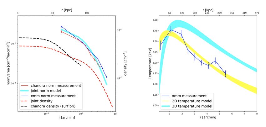
Fig. 9: The normalization (top), temperature (middle), and metallicity (bottom) profiles of the Northern Clump derived in the energy band 0.7−7.0
keV. Left: Southern region profiles. The blue and red data points represent XMM-Newton and Chandra, respectively. Right: Western region profiles.
The cyan and magenta data points represent XMM-Newton and Chandra, respectively. Due to modest photon counts, Chandra metallicity could
not be constrained in any sectors. The central data points fitted with AGN component are shown in grey, light green and dark green. These data
points are shifted for visualization purposes. The grey dashed lines indicate the R2500 of the cluster. The x-axis error bars are not the 1σ error range,
but the full width of the bins.
3.3. Spectral Analysis Table 4: eROSITA and XMM-Newton cluster parameters from the
kB T 500 region (0.2 − 0.5R500 ).
3.3.1. eROSITA Cluster Parameters
We list the eROSITA cluster parameters for the kB T 500 region (an norm† kB T Z
Instrument
annulus of 2.4 − 6.00 ) in Table 4. The metallicity returned by [keV] [Z ]
eROSITA is consistent with the one returned by XMM-Newton, full energy band∗
both in the wide and the small soft energy band, while the eROSITA 1.59+0.17
−0.19 1.67+0.20
−0.11
+0.11
0.36−0.12
normalizations and temperatures are lower. Fitting in the soft
band does improve the consistency between eROSITA and XMM- XMM-Newton 2.35+0.046
−0.045 1.99 ± 0.04 0.31+0.025
−0.026
Newton temperatures while not fully solving the discrepancies. 0.8 − 2.0 keV
While this could be an effect of instrumental calibration uncer- eROSITA 1.62+0.26 1.70+0.22 +0.19
0.36−0.14
tainties, it could also be caused by multi-temperature structure. −0.23 −0.11
As predicted by simulations, in the case of multi-temperature XMM-Newton 2.45+0.053
−0.052 1.99+0.050
−0.054 0.27+0.027
−0.025
plasma eROSITA that has superior soft response was shown to
return lower temperatures in comparison to other instruments
†
[10−5 cm−5 /arcmin2 ]
∗
(Reiprich et al. 2013). Fitting in the soft band only should 0.7/0.8 − 9.0 keV for eROSITA TM8/TM9.
minimize such effects as the relative effective areas are sim- 0.7 − 7.0 keV for XMM-Newton
ilar in this range for eROSITA and XMM-Newton. This issue
will be addressed further in the future, employing also eROSITA
mock observations based on hydrodynamical simulations, and 3.3.2. Inner of South and West
divising methodologies similar to the algorithm suggested by We plot the results of the spectral analysis of XMM-Newton and
Vikhlinin (2006) to predict the temperature in the case of multi- Chandra in the south and west directions of the Northern Clump
temperature plasma. in Figure 9 left and right panel, respectively. The top, middle,
and bottom panels are the normalization per area, temperature,
and metallicity profiles. Due to modest photon counts, the metal-
licities in Chandra can only be constrained using bins of full
azimuthal direction. The profile can be found in Appendix D,
Article number, page 12 of 24Angie Veronica et al.: The eROSITA View of the Abell 3391/95 Field: The Northern Clump
Figure D.2. The information regarding the source regions and are 56 (75)% and 83 (97)% higher, respectively. From XMM-
their best-fit parameter values are listed in Table D.2. Newton residual image (Figure 6, right), we estimated that the
In both directions, we observe a flattening towards the cen- excess emission in the north associated with the tail feature is
tral region of the cluster. The temperature profile towards the located at ∼ 70 (419.16 kpc) from the center and stretched out to
south indicates an elevated temperature around 20 < r < 30 12.50 (733.53 kpc). Therefore, we see an agreement between the
(119.76 kpc < r < 179.64 kpc). The metalicity also appears en- imaging and spectral analyses results. This tail feature is often
hanced in this region. Beyond the fourth bin, the temperature observed in other merging systems as a result of ram pressure
profile flattens at an average temperature of 1.94 keV. stripping. For example, the tail from M86 and M49 as they fall
into the Virgo Cluster (Randall et al. 2008; Su et al. 2019. Also
see Su et al. 2014, 2017a,b), the northeast tail feature observed
3.3.3. Outskirts of North, South, and West
in A2142 cluster (Eckert et al. 2014. Further confirmed through
dynamical study of the member galaxies in Liu et al. 2018), and
300 400
r [kpc]
500 600 700
a more extreme case of complete stripping is observed in the
galaxy cluster Zwicky 8338 (Schellenberger & Reiprich 2015).
In the south, higher temperature in comparison to the other
norm/area [cm 5/arcmin2]
10 5
two directions is apparent. At 11.250 (673.65 kpc), the tempera-
ture in the south is higher by 42 (20)% than in the north (west).
This elevated temperature may be associated with shock or com-
10 6
pression heated gas as the Northern Clump falls towards the
(0.7 - 7) keV south, into the A3391 cluster. At 5.00 (299.4 kpc), the normal-
XMM, North ization per area is higher than the other two directions, which is
XMM, South
XMM, West in agreement with the residual image (Figure 6, right) and the
10 7
4 5 6 7 8 9 10 11 12- 7) keV
(0.7
XMM, North
southern S X profile (Figure 7, right).
3.0 XMM, West The properties of the outskirts of the Northern Clump are
XMM, South
2.5 similar to those systems listed above, particularly the case of
kBT [keV]
M49 group residing beyond the virial radius of the Virgo Clus-
2.0
ter (Su et al. 2019). In addition to the stripped tail, a tempera-
1.5 ture enhancement is noted in front of the cold front in M49, re-
1.0 sembling the temperature elevation and surface brightness edge
(see Subsection 3.2.2) observed at ∼ 11.250 (673.65 kpc) and 50
0.5 4 5 6 7 8 9 10 11 12- 7) keV (299.4 kpc), respectively in the south of the Northern Clump.
(0.7
0.7 XMM, North
Our findings indicate that the Northern Clump may be undergo-
XMM, South
0.6 XMM, West
ing the same infalling process with M49.
0.5
Z [Z ]
0.4
0.3 3.3.4. Central AGN
0.2
We notice a metallicity drop in the core of the Northern Clump.
0.1
While it is commonly believed that this phenomena, which is of-
0.0
4 5 6 7 8 9 10 11 12 ten observed in galaxy groups and clusters with X-ray cavities,
r [arcmin] is the result of the AGN mechanical feedback and/or depletion
of Fe on to cold dust grains (Panagoulia et al. 2015; Lakhchaura
Fig. 10: XMM-Newton normalization (top), temperature (middle), and et al. 2019; Liu et al. 2019), it could also be an artefact that sur-
metallicity (bottom) profiles of the outer regions of the Northern Clump faces as the central AGN is not accounted properly in the spectral
in the different directions in the energy band 0.7−7.0 keV. The northern,
fitting (Mernier et al. 2017). To investigate this, we therefore im-
southern, and western regions are represented by orange, blue, and red
data points, respectively. The grey dashed (dotted) lines indicate the plement the second and third fitting methods (Subsection 2.2.2).
R2500 (R500 ) of the cluster. The x-axis error bars are not the 1σ error We present the best-fit parameter values of the three methods in
range, but the full width of the bins. The metallicity in the last two bins Table D.1 and the spectra with their best-fit model are displayed
of the south and west has been frozen to 0.3Z . in Figure D.3.
Since the on-axis Encircled Energy Fraction (EEF) for
We compare spectral properties of the north, south, and MOS1 camera is 68% at a 1500 radius4 , this indicates that there
west directions over R2500 to R500 (r = 4 − 12.50 = 239.52 − might be some AGN emission left in the source region while
733.53 kpc) as shown in Figure 10. We compare only XMM- performing the fit using the first method. While 92% of the to-
Newton values since, unfortunately, the outer north of the North- tal energy are encircled within a 6000 radius, having a mask of
ern Clump is not covered by the Chandra observations. We find this size in the core region is undesirable. The second and third
it necessary to fix the metallicity in the last two bins of the south methods are a better solution to this problem. However, as no-
and west to 0.3Z . The best-fit temperatures and normalizations ticed from the metallicity profiles, the low metallicity persists
vary within 1σ when we fix the metallicity of south and west to even when the AGN component is added.
the best-fit value of the north or fix the metallicity of the north to The apparent low core metallicity is better explained by
0.3Z . In general, our treatment of metallicity does not change the above-mentioned mechanical processes, for instance by the
the following results. AGN feedback, through which a fraction of the core metal-rich
We note a higher normalization per area in the last two bins ICM gas is distributed outwards (Sanders et al. 2016; Mernier
of the northern region. In comparison to the south (west) third 4
XMM-Newton Science Analysis System: Encircled energy
and fourth data points, the normalization per area in the north function
Article number, page 13 of 24You can also read