Petersen, G., Niemz, P., Cesca, S., Mouslopoulou, V., Bocchini, G. M. (2021): Clusty, the waveform-based network similarity clustering toolbox: ...
←
→
Page content transcription
If your browser does not render page correctly, please read the page content below
Petersen, G., Niemz, P., Cesca, S., Mouslopoulou, V., Bocchini, G.
M. (2021): Clusty, the waveform-based network similarity
clustering toolbox: concept and application to image complex
faulting offshore Zakynthos (Greece). - Geophysical Journal
International, 224, 3, 2044-2059.

https://doi.org/10.1093/gji/ggaa568

Institional Repository GFZpublic: https://gfzpublic.gfz-potsdam.de/
Geophys. J. Int. (2021) 224, 2044–2059                                                                                         doi: 10.1093/gji/ggaa568
Advance Access publication 2020 November 25
GJI Seismology

Clusty, the waveform-based network similarity clustering toolbox:
concept and application to image complex faulting offshore
Zakynthos (Greece)

                                                                                                                                                          Downloaded from https://academic.oup.com/gji/article/224/3/2044/6006268 by Geoforschungszentrum Potsdam user on 01 February 2021
G.M. Petersen,1,2 P. Niemz ,1,2 S. Cesca,1 V. Mouslopoulou3 and G.M. Bocchini                                                             4
1 GFZ  German Research Centre for Geosciences, Potsdam, Germany. E-mail: gesap@gfz-potsdam.de
2 Institute
          of Geosciences, University of Potsdam, Potsdam, Germany
3 National Observatory of Athens, Institute of Geodynamics, Athens 11810, Greece
4 Ruhr University of Bochum, Institute of Geology, Mineralogy and Geophysics, Germany

Accepted 2020 November 23. Received 2020 November 10; in original form 2020 July 30

                                     SUMMARY
                                     Clusty is a new open source toolbox dedicated to earthquake clustering based on waveforms
                                     recorded across a network of seismic stations. Its main application is the study of active faults
                                     and the detection and characterization of faults and fault networks. By using a density-based
                                     clustering approach, earthquakes pertaining to a common fault can be recognized even over
                                     long fault segments, and the first-order geometry and extent of active faults can be inferred.
                                     Clusty implements multiple techniques to compute a waveform based network similarity
                                     from maximum cross-correlation coefficients at multiple stations. The clustering procedure is
                                     designed to be transparent and parameters can be easily tuned. It is supported by a number
                                     of analysis visualization tools which help to assess the homogeneity within each cluster and
                                     the differences among distinct clusters. The toolbox returns graphical representations of the
                                     results. A list of representative events and stacked waveforms facilitate further analyses like
                                     moment tensor inversion. Results obtained in various frequency bands can be combined to
                                     account for large magnitude ranges. Thanks to the simple configuration, the toolbox is easily
                                     adaptable to new data sets and to large magnitude ranges. To show the potential of our new
                                     toolbox, we apply Clusty to the aftershock sequence of the Mw 6.9 25 October 2018 Zakynthos
                                     (Greece) Earthquake. Thanks to the complex tectonic setting at the western termination of the
                                     Hellenic Subduction System where multiple faults and faulting styles operate simultaneously,
                                     the Zakynthos data set provides an ideal case-study for our clustering analysis toolbox. Our
                                     results support the activation of several faults and provide insight into the geometry of faults
                                     or fault segments. We identify two large thrust faulting clusters in the vicinity of the main
                                     shock and multiple strike-slip clusters to the east, west and south of these clusters. Despite
                                     its location within the largest thrust cluster, the main shock does not show a high waveform
                                     similarity to any of the clusters. This is consistent with the results of other studies suggesting a
                                     complex failure mechanism for the main shock. We propose the existence of conjugated strike-
                                     slip faults in the south of the study area. Our waveform similarity based clustering toolbox is
                                     able to reveal distinct event clusters which cannot be discriminated based on locations and/or
                                     timing only. Additionally, the clustering results allows distinction between fault and auxiliary
                                     planes of focal mechanisms and to associate them to known active faults.
                                     Key words: Persistence, memory, correlations, clustering; Seismicity and tectonics; Frac-
                                     tures, faults, and high strain deformation zones.

                                                                               spatial and temporal seismicity patterns in great detail. In gen-
1 I N T RO D U C T I O N
                                                                               eral, earthquakes occur along pre-existing faults. Both, the extent
The world-wide increasing number of seismic stations, even de-                 and the stress state of seismogenic faults are of interest for struc-
ployed in areas of moderate seismicity, significantly lowers earth-            tural studies and for seismic hazard assessment at local, regional or
quake detection thresholds. This enables seismologists to study                global scale. The association of seismic events to faults is a major

2044
                                              C   The Author(s) 2020. Published by Oxford University Press on behalf of The Royal Astronomical Society.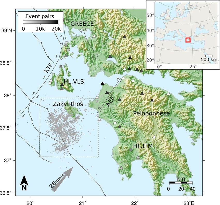
Waveform-based clustering offshore Zakynthos                 2045

but also challenging task. Depending on the location of active faults,     Shearer et al. 2005; Trugman & Shearer 2017). High waveform
fault identification may involve field investigations (i.e. mapping,       similarities among a small magnitude foreshock or afterhock with
trenching, etc.), aerial investigations (analysis of satellite images      a larger main shock with a known focal mechanism can be used to
or air-born lidar) or seismic-reflection/bathymetric data. Following       infer a similar mechanism for the weaker event. Such analyses can
large-magnitude earthquakes (Mw > 6), the geometry of the fault            also be used for a more advanced declustering of a catalogue, not
associated with the main rupture, as well as its slip distribution, is     only relying on occurrence times (Barani et al. 2007), as well as for
often estimated using seismological and geodetic tools (e.g. Koper         determining event pairs for an empirical green’s function analysis.
et al. 2011; Yokota et al. 2011; Grandin et al. 2015; Cirella et al.          Here we use a density-based clustering approach, which allows
2020).                                                                     grouping earthquakes with a wide range of magnitudes, locations
   Moment tensor inversion represents a powerful tool to identify          and focal mechanisms. End members of a density-cluster are not

                                                                                                                                                     Downloaded from https://academic.oup.com/gji/article/224/3/2044/6006268 by Geoforschungszentrum Potsdam user on 01 February 2021
earthquake faulting mechanisms. Focal mechanisms obtained for              required to be as similar as neighbouring events, if they are con-
seismic sequences are often used to obtain insight into the faulting       nected via multiple events with gradually changing locations or
style and the extent of an active fault (e.g. Örgülü & Aktar 2001;      mechanisms. Consequently, we are able to assign individual earth-
Serpetsidaki et al. 2010; Asano et al. 2011; Herrmann et al. 2011)         quakes assumed to be produced along an elongated fault into a
or the geometry of multiple faults (e.g. Cesca et al. 2017). Although      single cluster.
moment tensor inversion provides valuable insights, it has several            Here, we introduce a new open-source, user-friendly and highly
limitations that complicate the identification of active faults. First,    adaptable waveform clustering toolbox, named Clusty. The tool-
robust moment tensor inversions require a detailed knowledge of            box allows correlating and clustering hundreds to few thousands of
velocity structures and station instrumentation. Furthermore, the          events recorded by a network of stations based on what we refer to
quality of moment tensor solutions strongly depends on the radiated        as the network similarity of the event pairs. We implemented dif-
frequencies: for lower magnitude events moment tensor inversion            ferent approaches to combine the waveform similarities computed
is often not feasible. In these cases, the signal to noise ratio is only   for multiple stations across a network, allowing a comparison of the
sufficient at higher frequencies which cannot be modelled using            clustering methods and their results. In the development of the code
simple 1-D velocity models. Finally, the causative fault plane cannot      we put emphasis not only on computational efficiency and the sta-
be distinguished from the auxiliary plane of the moment tensor (MT)        bility of results, but also on a broad range of analysis and plotting
without additional geological (e.g. fault geometry) or geophysical         tools. Apart from the resulting catalogue of clustered events and
constraints (e.g. GPS displacements or aftershock distributions).          accompanying plots, Clusty provides a list of representative events,
   The clustering of earthquakes into groups of similar events is an-      i.e. one event for each cluster that is most similar to the rest of the
other approach to analyse the observed seismicity regarding under-         cluster. The representative events can be used to perform moment
lying seismogenic processes. The clustering analysis can be based          tensor inversions aiming for a representative focal mechanism for
on various parameters such as: (1) spatial and/or temporal distribu-       each cluster.
tions (e.g. Frohlich 1987; Shearer et al. 2005; Ansari et al. 2009;           In this study we apply the clustering toolbox to the aftershock
Ouillon & Sornette 2011; Mouslopoulou & Hristopulos 2011; Mes-             sequence of the 25 October 2018 Mw 6.9 Zakynthos (Greece) earth-
imeri et al. 2019; Czecze & Bondár 2019); (2) the smallest rotation       quake (Chousianitis & Konca 2019; Cirella et al. 2020; Ganas et al.
between moment tensors (e.g. Cesca 2020); (3) P and S polarities           2020; Karakostas et al. 2020; Mouslopoulou et al. 2020; Sokos et al.
(e.g. Shelly et al. 2016) or (4) waveform similarities, as for exam-       2020). The data set includes >2300 events with M ≥ 2.8 recorded at
ple in Tsujiura (1983), Maurer & Deichmann (1995), Shearer et al.          33 stations from 25/10/2018 to 14/11/2019. The catalogue is avail-
(2003), Barani et al. (2007), Trugman & Shearer (2017), Ruscic             able in Mouslopoulou et al. (2020). Zakynthos is located in the prox-
et al. (2019), Abramenkov et al. (2020) and in this study.                 imity of the western termination of the Hellenic subduction zone.
   The clustering based on waveform similarity favours fault map-          The region is known for its high seismic activity and a great variety
ping by considering locations and mechanisms, since waveforms              of faulting mechanisms (Mouslopoulou et al. 2020). Serpetsidaki
are inherently sensitive to both. Waveform similarity is generally         et al. (2010) studied another seismic sequence offshore Zakynthos
assessed by cross-correlating waveforms of earthquakes at one or           in April 2006 and emphasized the importance of the identifica-
multiple stations. Very high waveform similarities (i.e. >0.9–0.95)        tion of active faults for regional seismic hazard assessment. Our
are attributed to so-called repeaters (e.g. Geller & Mueller 1980;         waveform-based clustering analysis provides a better understand-
Igarashi et al. 2003; Baisch et al. 2008; Han et al. 2014). According      ing of the geometries and kinematics of the faults involved in the
to Geller & Mueller (1980) repeaters are located at distances smaller      2018–2019 aftershock sequence. Further, we associate moment ten-
than a quarter of the dominant wavelength, however, also larger            sors inverted for representative events to the individual clusters. The
spatial separation was reported (e.g. Arrowsmith & Eisner 2006).           identification of different waveforms excited by spatially clustered
Similar waveforms, observed at multiple stations, imply similar fo-        earthquakes provides evidence for the presence of various faulting
cal mechanisms and travel paths (locations and depths, e.g. Maurer         styles on neighbouring faults, an outcome that is in agreement with
& Deichmann 1995). Thus, the identification of clusters of similar         the local geology (Mouslopoulou et al. 2020) and the regional stress
events can shed light on the fault geometry and on the faulting style.     field (Konstantinou et al. 2017).
In favourable conditions, waveform similarity studies can help to             We use the Zakynthos application to assess the stability of the
identify faults and map their geometries (e.g. Tsujiura 1983; Maurer       clustering results, using different clustering settings, frequency
& Deichmann 1995; Shearer et al. 2003). The waveform similarity            ranges and discuss limits and opportunities of the toolbox. In Sec-
based clustering approach is independent from the uncertainty of           tion 2, we describe the work-flow of the clustering toolbox Clusty.
the hypocentral locations, therefore it can be applied even when           We applied our toolbox to the Zakynthos Earthquake aftershock case
hypocentral locations are poorly constraint. Only at a later stage of      study and present the results of the clustering analysis in Section 3.
this study, when fault planes are inferred from the clusters, the loca-    We discuss both, the methods and the application with respect to
tion uncertainties are considered. Waveform similarity is also used        the clustering results, inferred fault geometries and methodological
to identify groups of events for relative relocation methods (e.g.         limitations in Section 4.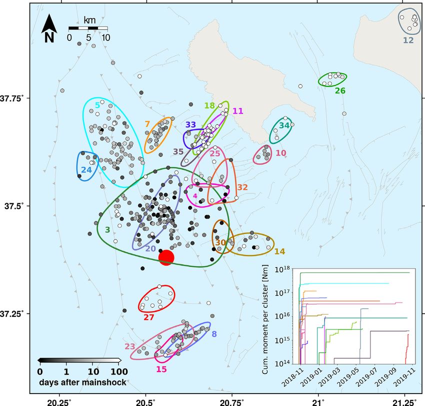
2046      G.M. Petersen et al.

                                                                        for layered earth models (Heimann et al. 2017). The user can ei-
                                                                        ther select a fixed time window for each phase or use our empirical
                                                                        relations (i.e. for surface waves: [tonset − 10s, tonset + (3/fmin ) +
                                                                        10s] and for body waves: P: [tP − 2, tS ], S: [tS − 2, 1.5(tS − tP )]).
                                                                        Clusty preprocesses the waveforms, that is downsampling and band-
                                                                        pass filtering, and applies thresholds for inter-event distances (either
                                                                        epicentral (in this study) or hypocentral), event-to-station distances
                                                                        and signal-to-noise ratio (SNR). While none of these thresholds are
                                                                        strictly required, we recommend using them for computational ef-
                                                                        ficiency. Distance-based thresholds should be set conservatively to

                                                                                                                                                   Downloaded from https://academic.oup.com/gji/article/224/3/2044/6006268 by Geoforschungszentrum Potsdam user on 01 February 2021
                                                                        avoid rejecting event pairs or station-event-pairs due to mislocated
                                                                        events. A minimum station–event distance is recommended as the
                                                                        clustering method assumes a station–event distance that is large
                                                                        compared to the event–event distance.
                                                                           The workflow can be quickly adjusted to three channel or single
                                                                        channel data. For all event pairs passing the thresholds, Clusty com-
                                                                        putes the maximum cross-correlation coefficient (cc) at each sta-
                                                                        tion and for each component. For computational efficiency, this step
                                                                        runs in parallel on a user-defined number of cores on the CPU. Only
                                                                        event-pairs, that exceed an additional cc threshold (e.g. >0.7) at a
                                                                        minimum number of stations (e.g. >5), with a minimum azimuthal
                                                                        station coverage (e.g. >60◦ ) are considered in the subsequent analy-
                                                                        sis. However, it is important to notice that once these conditions are
                                                                        satisfied, all stations which passed the primary SNR and distance
                                                                        thresholds (and not only those passing the cc threshold) will be
                                                                        considered for the network similarity computation to assure that the
                                                                        statistics are not biased. The cc threshold does not represent a mea-
                                                                        sure of the minimum similarity among events in the later applied
                                                                        clustering process. It only assures higher computational efficiency.
                                                                           By applying the above mentioned thresholds, we reduced the
                                                                        number of calculated cross-correlations in our test data set from
                                                                        more than 378 million (45 stations, 3 components, 2367 events)
                                                                        to about 5 million. The pre-processing of the waveforms and the
                                                                        calculation of the cc values is the computationally most expensive
                                                                        step within Clusty. In the frequency band of 0.05–0.20 Hz (allowing
                                                                        a downsampling to 10 Hz) it takes about 4 hr on a cluster using 16
                                                                        cores. All further steps within Clusty require only a few minutes on
                                                                        a single core. A memory saving option is available, so that Clusty
                                                                        can also be used on personal computers.
                                                                           The cc values of the event pairs at each station are combined to
                                                                        a network similarity for each component using one of the methods
                                                                        described below. Subsequently, the components can be combined or
                                                                        analysed individually, for example to compare the results obtained
                                                                        from horizontal and vertical components. The network similarity
Figure 1. Schematic workflow diagram for the waveform-based network     matrix is then used as input for the clustering algorithm DBSCAN
similarity clustering toolbox Clusty.                                   (Ester et al. 1996, see Section 2.2). The choice of appropriate clus-
                                                                        tering parameters is often difficult and sometimes subjective. To
                                                                        overcome these difficulties we implemented tools for testing vari-
                                                                        ous sets of clustering parameters and compare them using multiple
2 M E T H O D O L O G Y: T H E C L U S T Y
                                                                        analysis plots (see Section 2.3).
N E T WO R K S I M I L A R I T Y C LU S T E R I N G
                                                                           To analyse earthquakes with a broad range of magnitudes, the
TO O L B OX
                                                                        entire workflow can be repeated using different frequency bands.
Clusty is a flexible, efficient and user-friendly python toolbox ded-   The resulting cluster labels can be harmonized with respect to a
icated to seismic cluster analysis based on waveform similarity         defined reference frequency band to create a joint cluster result
across a network of stations. It is based on the seismological python   catalogue. The user can run Clusty in one flow, but tuning the
library Pyrocko (Heimann et al. 2017) and is running on Linux           settings of the network similarity computation and the clustering
systems including desktop and server environments.                      parameters is a crucial point in this analysis. Therefore all steps
   The general workflow is sketched in Fig. 1. As input Clusty          can be run separately and repeated (e.g. computation of cc, network
requires an earthquake catalogue, waveform data and station meta-       similarity, clustering, plotting of the results).
data. If phase picks are not available, it is possible to compute          Settings for the toolbox like frequency filters, downsampling,
theoretical arrival times using a chosen 1-D velocity model and         SNR thresholds to retain or reject events as well as the choice
cake, a tool implemented in Pyrocko to solve ray theory problems        of methods to compute the network similarity can be defined in a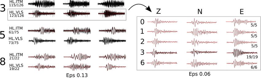
Waveform-based clustering offshore Zakynthos                 2047

configuration file. We provide an example configuration file in the git    However, we recommend to use a threshold for a required cc value
repository including information on the settings used for this study       at a minimum number of stations. Further, the resulting weights
(https://git.pyrocko.org/clusty/clusty, last accessed October 2020).       should be analysed along with the network similarity to avoid that
Clusty returns several figures to evaluate and present the results         the result is dominated by few stations only.
together with the output from the cluster analysis (i.e. clustering           Another approach to combine the cc values of all stations is a
matrices and event-cluster identification). In addition, Clusty can        composite correlation measure computed as the Mth root of the
provide stacked waveforms for each cluster as well as a list of            product of the cc values (Stuermer et al. 2011):
representative events for subsequent studies.

                                                                                            M
                                                                           nsim i j,c = [     (cci j,c,s )]−M .                               (3)

                                                                                                                                                     Downloaded from https://academic.oup.com/gji/article/224/3/2044/6006268 by Geoforschungszentrum Potsdam user on 01 February 2021
                                                                                            s=1
2.1 Network similarity computation
                                                                           Stuermer et al. (2011) combined P and S cc values extracted from
The network similarity nsim of two events with index i and j (event
                                                                           the same single component trace in the product. When using three
pair ij) across a network of stations s with components c can be com-
                                                                           component data, we first compute the Mth root of the product for
puted based on the maximum cross-correlation coefficients ccij,c,s
                                                                           each component c separately, and then combine the obtained net-
using a variety of methods implemented within the clustering tool-
                                                                           work similarities in a consecutive step.
box to allow an easy comparison of different techniques. The net-
                                                                              The network similarity matrices nsimij,c are computed for the
work similarity of each event-pair is a value between 0 and 1, with
                                                                           different components c (e.g. Z, N and E) separately and subsequently
1 being the highest correlation.
                                                                           combined as a weighted sum:
   For each pair of events i, j the maximum, the mean or the median
of the ccij,c,s value of all stations s (separate components c) can,
                                                                                        C

among other methods, be used as a measure for network similarity.          nsim i j =         nsim i j,c ωc .                                 (4)
These three methods are computationally very efficient. However,                        c=1

the mean of the cc values of all stations is generally prone to outliers   The weighting of the components ωc is defined in the configura-
especially when calculated from a small sample of events, while the        tion file. A component-based weighting allows compensating site-
maximum of the cc values can be distorted in case of highly corre-         effects, which can lead to complex horizontal traces. The weighting
lated monotonous noise or band-limited stations, for example due           can also compensate for variations in waveforms originating from
to high near-surface attenuation (Aster & Scott 1993). Moreover,           different mechanisms that affect horizontal and vertical components
the maximum-method is based on the cc value of a single station            differently. By comparing the results of independent phases (e.g. P
and cannot separate two different mechanisms which may radiate             and S or Love and Rayleigh) and components (i.e. Z, N and E)
similar, highly correlated waveforms in the particular direction of        one can learn about the sensitivity of the waveforms in regard to
the station. Therefore Aster & Scott (1993) suggest using the me-          different faulting types.
dian of the cc values of all stations as best practice to determine the
degree of similarity between two events. Consequently, the maxi-
mum value should only be used for testing, to adjust time windows          2.2 Event clustering
and select appropriate bandpass filters or in cases where only single
stations close to the epicentre have a sufficient SNR (Ruscic et al.       For the clustering algorithm input, the network similarity matrix
2019). For smaller magnitudes only the closest stations are expected       (with 1 being the highest correlation) is converted into a distance
to record an event, therefore it helps to use the mean or median of        matrix (with 0 corresponding to identical events). To avoid con-
those stations that comply with the given SNR threshold.                   fusion with the spatial distance we hereafter refer to it as the
   For the same reason Maurer & Deichmann (1995) introduced an             similarity-distance. At the current version of the clustering tool-
asymmetrically trimmed mean for the computation of the network             box, the density-based DBSCAN algorithm (Ester et al. 1996), as
similarity nsimij,c across a total number of M stations: For each event    implemented in the python package scikit-learn (Pedregosa et al.
pair the lowest k per cent of the cc values are removed before the         2011), is used for clustering. Other clustering algorithms, such as
mean is computed:                                                          OPTICS (Ankerst et al. 1999) or k-means (Lloyd 1982) can be
                                                                           added by the user depending on the clustering targets.
                  1    M
                      M−k
                                                                               Clusters derived using the DBSCAN algorithm can have any
nsim i j,c =               cci j,c,s ,                              (1)
               M − k M s=1                                                 shape and the number of clusters is not predefined. Further, the
                                                                           algorithm allows for unclustered events (a noise class). Following
where ccij,c,s is sorted by descending cc value. Lower cc values
                                                                           the definitions of Ester et al. (1996), events belonging to one cluster
between events at some stations do not necessarily imply weaker
                                                                           are either core events or border events. Core events have at least
correlation of the events in regard to mechanism and location but
                                                                           a minimum number of neighbouring events (MinPts) within the
can also be caused by other influences, such as variable site effects
                                                                           similarity-distance Eps. Events at the border of the cluster (bor-
or noise conditions (Akuhara & Mochizuki 2014).
                                                                           der events) are connected to at least one core point, but have less
   The network similarity of an event pair can also be computed as
                                                                           then MinPts neighbouring events within the similarity-distance Eps.
a weighted sum of the cc values at all stations. The weights wij,c,s are
                                                                           Clusters are formed based on the concept of density reachability. An
the absolute differences between the first and the second maximum
                                                                           event i is considered directly density-reachable from a core event j,
of the according cross-correlation function (Shelly et al. 2016):
                                                                           if it is within the similarity-distance Eps. Further the events i and j

               M                                                           are density-connected if they are density-reachable through one or
nsim i j,c =         cci j,c,s wi j,c,s .                           (2)    more density-connected core events.
               s=1                                                             The DBSCAN clustering procedure starts with the selection of an
The use of a weighted sum limits the influence of poorly correlated        arbitrary event of the data set. All events that are density-reachable
records from distant or noisy stations and stabilizes the computation.     from this very first event (with respect to Eps and MinPts) are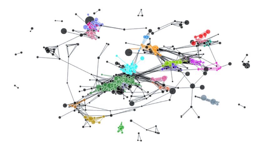
2048 G.M. Petersen et al.
retrieved. A cluster is only formed if there is at least one core event. reflect the ensemble of all clusters, while the influence of differ-
If not, DBSCAN visits the next point of the database. This process ent parameter sets onto single clusters can be analysed using more
is continued until all points have been processed (Ester et al. 1996). sophisticated analysis tools, introduced hereafter. Fig. 2(b) shows
Events not lying within similarity-distance Eps of any other event these metrics for Eps values between 0.01 and 0.30 and MinPtS
are assigned to a noise class (unclustered). Eps and MinPts need to values of 5 and 8. The trends of the three curves are similar for both
be tuned by the user according to the data set. MinPts values. The silhouette score is a measure of the homogeneity
of all clusters (Rousseeuw 1987), here neglecting the unclustered
events. It is the mean of the silhouette coefficients of all clustered
events. The silhouette coefficient of a single event expresses how
similar that event is compared to the other events within the same
Downloaded from https://academic.oup.com/gji/article/224/3/2044/6006268 by Geoforschungszentrum Potsdam user on 01 February 2021
2.3 Tuning of the clustering parameters and graphical
cluster and compared to the events of the nearest other cluster. The
analysis of clustering results
silhouette coefficient is defined as:
Our clustering toolbox provides several analysis plots that facilitate
s = (icd − ncd)/max(icd, ncd), (5)
the tuning of the clustering parameters and the evaluation of the
stability of the clusters. Further, these plots provide detailed insight where ncd is the mean nearest cluster similarity-distance for
into the clustering results. The plotting tools can also be used to each event and icd is the mean intracluster similarity-distance
analyse, compare and choose multiple target frequency bands to (Rousseeuw 1987). The silhouette coefficient ranges between –1
include surface waves for larger, distant events and body waves for and 1, where 1 corresponds to a cluster of identical events, that
smaller, local events. The graphical output is generated using GMT are completely different from events belonging to other clusters.
(Wessel et al. 2013) and the python plotting packages matplotlib Coefficients between –1 and 0 indicate that the similarity-distance
(Hunter 2007) and plotly (Plotly Technologies Inc. 2015). The plots of an event with respect to events of other clusters is smaller than
presented in this section illustrate the analysis that was performed the average similarity-distance to events of its own cluster. We use
to obtain optimal clustering settings and stable results for the appli- the implementation of scikit-learn (Pedregosa et al. 2011) to cal-
cation to the aftershock sequence of the 25 October 2018 Zakynthos culate the silhouette coefficients. The silhouette score in Fig. 2(b)
Mw 6.9 earthquake in Greece. is largest at very low Eps values, when only highly similar earth-
Clusty allows the user to run the entire clustering process for quakes are assigned to one or few clusters. Thereafter, the silhouette
different DBSCAN parameters (Eps and MinPts) in parallel to com- score decreases with increasing Eps value, so in fact we are visually
pare the results. As mentioned above, the input similarity-distance searching for local maxima or changes in the gradient of the curve,
matrix for DBSCAN is computed from the cross-correlations of but not for the global maximum. The shift between the two lines
waveforms. Therefore the similarity-distance radius (Eps) is di- for MinPts 5 and 8 (grey and black, respectively) in Fig. 2(b) is the
rectly related to the underlying physical process and a rough first result of an increased number of earthquakes required per cluster for
estimate of Eps can be made based on expected similarities. How- higher MinPts values. The first cluster can therefore only be found
ever, the expected cc values, and consequently, the optimal Eps for a slightly higher Eps value in case of a higher MinPts value.
value may vary depending on the length of the considered wave- In both curves a local maximum is seen at an Eps value of 0.06.
form time windows, the frequency content as well as on site and Several minor changes in the gradient are observed between 0.10
noise conditions at the stations. An Eps of 0.1 implies that a pair of and 0.14, followed by a major gradient change at 0.15 (black arrow
connected events has at least a network similarity of 0.9. Depend- in Fig. 2b). Below Eps 0.15, the silhouette score is relatively stable
ing on the chosen method for the network similarity computation, on a low level. By decreasing the Eps only by 0.01 or 0.02 we ob-
waveform cross-correlation values at single stations can be smaller tain significantly higher silhouette scores, thus more homogeneous
if other stations with higher values compensate for it. Eps needs clusters (Fig. 2b), a prerequisite for a reliable identification of ac-
to be adjusted to the purpose of the clustering. Using a small Eps tive faults. The total number of clusters and the number of clustered
value allows finding very similar events or repeaters. However, in events decreases with increasing MinPts, resulting from a higher
this case other events are omitted, which would still be considered required number of earthquakes to form a cluster. The number of
similar when clustering is performed using a higher Eps for fault clustered events increases rapidly until an Eps value of 0.13 (MinPts
identification and tracing. 5, green arrow in Fig. 2b) and 0.16 (MinPts 8) and shows a smaller
Ester et al. (1996) suggested a k-nearest neighbour (k-NN) gradient afterwards. Local maxima of the number of clusters are
plot (Fig. 2a) to choose the Eps parameter. Therein, the average found for 0.10 and 0.13 (blue arrow in Fig. 2b) for MinPts 5 and
similarity-distance of every sample to its k nearest neighbours (here 0.13 for MinPts 8. For larger Eps values single clusters collapse into
corresponding to the MinPts parameter) is calculated and plotted larger, more heterogeneous ones, as can be seen in the flow diagram
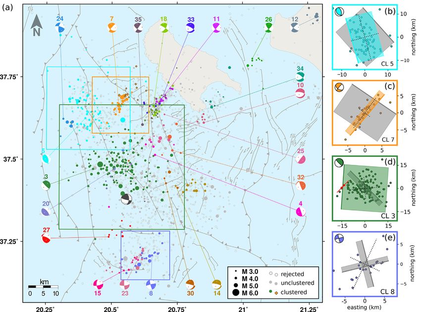
in an ascending order to visually find a ’knee’, that corresponds to (Fig. 3).
the optimal Eps value for the given data set (Ester et al. 1996). In The flow diagram helps to assess the stability of the clustering
Fig. 2(a), the sorted similarity-distances of the kth nearest neigh- results. It allows a comprehensive comparison of clustering results
bours are shown for MinPts values from 5 to 8. For MinPts 5, sig- obtained using different clustering parameters (Fig. 3) or waveform
nificant gradient changes are seen for Eps values of 0.16 and 0.21 frequency filters (Fig. S1). Fig. 3 shows the flow diagram of clus-
(red arrows in Fig. 2a). For increased MinPts values these gradient tering results obtained for an Eps range of 0.06–0.30. The width of
changes are observed for larger Eps values. However, we prefer the connecting bands between two clusters obtained with two sets
smaller Eps values, because otherwise we observe rather unstable of parameters is proportional to the number of common events. In
and heterogeneous clusters in our application (Fig. 2b and following this way, the diagram reflects conserved quantities as well as the
paragraphs). Therefore, we suggest three additional metrics to con- splitting or merging of clusters (Fig. 3). In Fig. 3 the small clusters
strain a range of appropriate DBSCAN clustering parameters for in the lower part of the diagram remain stable over a wide range
fault tracing purposes: (1) the silhouette score, (2) the number of of Eps values. The two largest and distinct green and light blue (3
clusters and (3) the total number of clustered events. These metrics and 5) clusters collapse into one heterogeneous cluster when Eps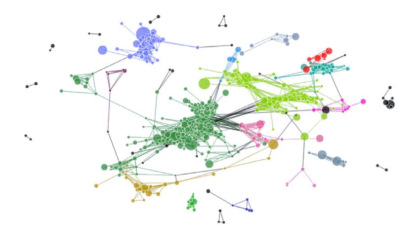
Waveform-based clustering offshore Zakynthos 2049
(a) (b)
Downloaded from https://academic.oup.com/gji/article/224/3/2044/6006268 by Geoforschungszentrum Potsdam user on 01 February 2021
Figure 2. Selection of the DBSCAN clustering parameters. (a) The k-nearest neighbour plot (here for MinPts of 5–8) helps selecting Eps by identify a ’knee’
(gradient changes, red arrows). (b) Silhouette score (black solid lines), number of clusters (blue dotted lines) and total number of clustered events (green
dashed lines) for Eps values between 0.01 and 0.4 and MinPts values of 5 (lighter colours) and 8 (darker colours). Arrows mark features discussed in the text
for MinPts 5. Blue: max. number of clusters, green: gradient change in number of clustered events, black: gradient change in silhouette score. Red dotted line
indicates the Eps value used in the application to the Zakynthos data set (0.13).
Figure 3. Screenshot of the interactive flow diagram for a comparison of clustering results obtained with Eps values between 0.06 and 0.30, MinPts 5
(0.05–0.2 Hz). Black represents the noise cluster (here reduced in size to emphasize the clustered events). Same colours represent the same cluster. The size of
the clusters varies depending on the required similarity (Eps value), the block size is proportional to the number of events within the cluster. The grey bands
connect clusters obtained with different clustering parameters which share at least one event. The thickness of the grey bands is proportional to the number of
shared events. This representation allows evaluating the stability of cluster results when changing clustering parameters.
increases from 0.14 to 0.15. For Eps values as small as 0.06 only few The silhouette coefficient plot (Figs 4a–c) shows how similar
small clusters are found. For Eps = 0.30 large clusters with clearly each event is to the events in its own cluster compared to the events
distinguishable event types (when using a smaller Eps) collapse into of the most similar cluster (Rousseeuw 1987). Each coloured block
one cluster. represents the events of one cluster, sorted by their silhouette coef-
When using multiple clustering settings, the resulting clusters as ficient. The silhouette plot helps to find appropriate Eps and MinPts
well as their labels will differ. Therefore, we implemented a function settings and the optimal number of clusters by evaluating the simi-
that provides harmonized cluster labels across the different cluster- larity of events within each cluster. The connectivity plot (Figs 4d–f)
ing results. The harmonization of labels can lead to a discontinuous provides a complementary visualization of the similarity between
cluster label numbering but assures that labels are persistent. events as well as between clusters. Within this force-directed projec-
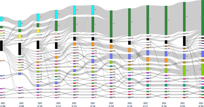
Finally, we introduce two more visualization tools to analyse tion (Fruchterman & Reingold 1991) the relative distance between
the clustering parameters and control the clustering results: the events or clusters of events represent their similarity. When choos-
silhouette coefficient plot (Figs 4a–c) and the event-connectivity ing Eps=0.06 (Figs 4a and d) only a few, very similar events are
plot (Figs 4d–f). Both depict the homogeneity and the connectivity clustered. However, the visualization of the connectivity (Fig. 4d)
within each cluster or among different clusters, respectively. shows that there are many more clusters of similar events. This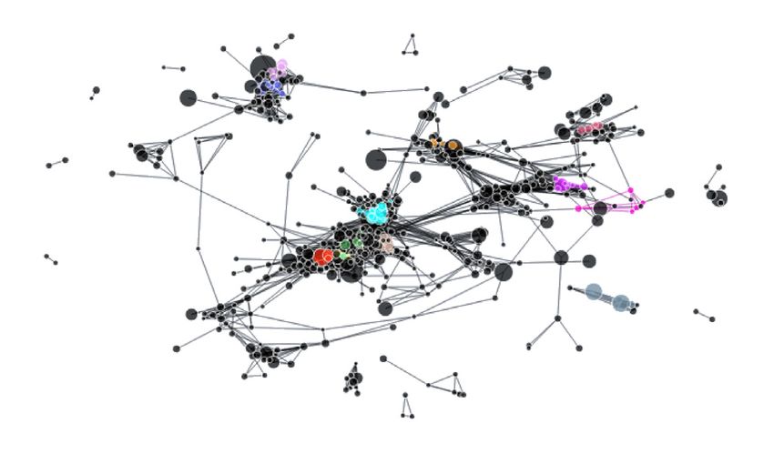
2050       G.M. Petersen et al.

             (a)                                                                  (d)

                                                                                                                                                                    Downloaded from https://academic.oup.com/gji/article/224/3/2044/6006268 by Geoforschungszentrum Potsdam user on 01 February 2021
             (b)                                                                  (e)

             (c)                                                                  (f)

Figure 4. Example for silhouette coefficient plots (a–c) and connectivity plots (d–f), obtained for the Zakynthos data set with Eps values 0.06, 0.13 and 0.3,
MinPts = 5. The numbers next to the clusters in (a–c) indicate the cluster label. The red vertical line is the silhouette score (mean of silhouette coefficients)
of the clustered events. The connectivity plots (d–f) provide an additional visualization of the similarity of events within the same cluster as well as among
different clusters. Events are coloured according to their cluster as in (a–c). Unclustered events are shown in black. In this projection the relative distance
between events or clusters represents their similarity. The absolute locations within the projection have no meaning.

cannot be seen from the silhouette plot alone (Fig. 4a). By increas-                with any other distance matrix provided by the user. For example,
ing Eps to 0.13 (Figs 4b and e) all clusters are well separated and                 these distance matrices could be based on Kagan angles or spatial
homogeneous, except for cluster 3 and 18. For Eps=0.30 (Figs 4c                     distances.
and f) the central clusters collapse into one. In the latter case, the
silhouette plot indicates that the clusters are generally more hetero-
geneous and larger. We want to stress the importance of the analysis                3 A P P L I C AT I O N : O F F S H O R E
of both, the similarity between separated clusters as well as among                 AFTERSHOCK SEQUENCE OF
the events that belong to the same cluster, before interpreting the                 T H E M 6 . 9 Z A K Y N T H O S E A RT H Q UA K E ,
results. The user can get insights into the quality of the performed                GREECE
clustering analysis by comparing the presented plots for a range of
parameters.                                                                         3.1 Study area
   Clusty provides maps and waveform plots as final graphical
                                                                                    The study area is located at the western margin of the Hellenic Sub-
output along with the catalogue of clustered events (for examples,
                                                                                    duction System (HSS), along which the oceanic lithosphere of the
see also Section 3). Station-wise waveform plots display all aligned
                                                                                    African Plate is subducted beneath the continental lithosphere of the
waveforms per cluster and component. The waveform plots provide
                                                                                    Eurasian Plate with a NE dipping slab (Fig. 5). Within the study area,
another direct visualization to evaluate the similarity of waveforms.
                                                                                    faults of varying geometries and slip movements (Mouslopoulou
We would like to point out that the clustering algorithm, the plots
                                                                                    et al. 2020) accommodate the northward kinematic transition from
to evaluate the stability of the results (flow diagram, silhouette and
                                                                                    convergence to strike-slip (i.e. Pérouse et al. 2017; Sachpazi et al.
connectivity plots) and the final maps may be used independently
Waveform-based clustering offshore Zakynthos 2051
Downloaded from https://academic.oup.com/gji/article/224/3/2044/6006268 by Geoforschungszentrum Potsdam user on 01 February 2021
Figure 5. Study area and station network. Triangles indicate seismic stations. Colour intensity depicts the contribution of each station to the clustering result
(number of clustered event pairs for which the station was used). The dashed square outlines the extent of Figs 6(a) and 7. The grey arrow indicates the relative
movement of the African Plate with respect to stable Eurasia (Pérouse et al. 2017). Active regional faults from Basilic et al. (2013), topography from SRTM
(Farr et al. 2007). KTF, Kefalonia Transform Fault; AEF, Achaia-Elia Fault.
2000). Although all types of faulting (thrust, normal and strike-slip) Our study is based on the catalogue of the aftershock se-
may occur (Konstantinou et al. 2017; Mouslopoulou et al. 2020), quence reported by Mouslopoulou et al. (2020). It consists of
thrust faulting appears to prevail south and southwest of Zakynthos ≥2300 events (Mw ≥2.8), including about 80 double-couple so-
(Papadimitriou et al. 2013; Wardell et al. 2014), while strike-slip lutions showing a large variability of thrust, normal and strike-slip
faulting is dominant to the northwest (Louvari et al. 1999; Sachpazi mechanisms. This hints at the activation of a complex fault sys-
et al. 2000), onshore Peloponnese (Feng et al. 2010; Stiros et al. tem, in accordance with local fault diversity (e.g. Konstantinou
2013) and in the offshore area between Zakynthos and Peloponnese et al. 2017; Mouslopoulou et al. 2020). Thanks to the complex
(Kokkalas et al. 2013; Haddad et al. 2020; Mouslopoulou et al. tectonic setting, together with the multitude of activated faults,
2020). Normal faulting is accommodated in the shallower sections we consider the Zakynthos data set an ideal case study for our
of the crust (above 15 km), often at high angles to the prevailing clustering analysis tool. The waveform data of the networks HA,
strike of the mapped thrust/strike-slip faults (Mouslopoulou et al. HC, HL, HP, HT, MN (University Of Athens 2008; Technologi-
2020). cal Educational Institute Of Crete 2006; National Observatory Of
The study region is characterized by intense seismic activity and Athens, I. O. G. 1997; University Of Patras, G. D. 2000; Aristo-
strong main shocks (M > 6, Papazachos & Papazachou 2003). On 25 tle University Of Thessaloniki Seismological Network 1981; Med-
October 2018, a magnitude Mw 6.9 earthquake struck southwest of Net Project Partner Institutions 1990) used in this study was ob-
Zakynthos (Chousianitis & Konca 2019; Cirella et al. 2020; Ganas tained using the pyrocko fdsn client to access the databases of
et al. 2020; Karakostas et al. 2020; Mouslopoulou et al. 2020; Sokos the National Observatory of Athens Seismic Network (NOA, http:
et al. 2020). It occurred after a 4-yr-long phase of seismic unrest //www.gein.noa.gr/en/), GEOFOrschungsNetz (GEOFON; https://
which was probably triggered by a slow-slip event (Mouslopoulou geof on.gfz-potsdam.de/), Observatories and Research Facilities for
et al. 2020) and was followed by strong aftershock activity, which European Seismology (ORFEUS; https://www.orfeus-eu.org/), In-
is still ongoing (Mouslopoulou et al. 2020; Sokos et al. 2020). corporated Research Institutions for Seismology (IRIS; https://ww
The complex moment tensor of the main shock, with a significant w.iris.edu/hq/) and Instituto Nazionale di Geofisica e Vulcanologia
non-double couple component, was attributed to subevents of thrust (INGV; http://webservices.ingv.it).
faulting and moderately dipping right lateral strike-slip faulting, in
accordance with the African–Eurasian Plate motion (Cirella et al.
2020; Mouslopoulou et al. 2020; Sokos et al. 2020). While seismo- 3.2 Results
logical results alone cannot clearly discriminate between a splay- Here, we present the clustering results for the Zakynthos data set
thrust and a subduction-thrust fault scenario for the main candidate obtained using a 30 per cent-trimmed mean for the calculation
earthquake fault, the scenario of a splay-thrust fault is supported by of the network similarity from waveforms of the seismic stations
published seismic-reflection and bathymetric data (Mouslopoulou presented in Fig. 5. Vertical (HHZ) and horizontal (HHN and HHE)
et al. 2020) and the recording of a minor tsunami that suggests components were combined with weightings of 0.4, 0.3 and 0.3,
rupture of the sea-bed (Cirella et al. 2020). respectively. Only event-pairs with cc values ≥0.7 and an SNR ≥ 22052 G.M. Petersen et al.
at more than five stations, covering a minimum azimuthal range of Due to the vicinity of these two clusters, the smaller strike-slip clus-
60◦ , are considered. We discuss the choice of the network similarity ter cannot be detected based on spatio-temporal clustering. While
computation method and the DBSCAN clustering parameters (here: the strike-slip clusters 7 and 24, which are located to the east and to
Eps 0.13, MinPts 5, primary frequency band 0.05–0.20 Hz, time the west of cluster 5, respectively, are active within the first ten days
window 80 s) in Section 4. after the main shock, the activity of the overlapping strike-slip clus-
We used four different frequency bands to account for surface ters 11, 18 and 35 starts two months later (Fig. 7). Cluster 33, which
waves (0.02–0.15 Hz and 0.05–0.20 Hz) and body waves (0.1– overlaps spatially with cluster 11, 18 and 35, in contrast is active
0.5 Hz and 0.2–1.0 Hz). The overall patterns of clustered events are within the first days after the main shock and shows a more oblique
similar in all four frequency bands. Considering the stability and mechanism (Fig. 6). South of the main shock, three spatially and
homogeneity as well as the total number of clustered events, the temporally overlapping strike-slip clusters (8, 15, 23) show a similar
Downloaded from https://academic.oup.com/gji/article/224/3/2044/6006268 by Geoforschungszentrum Potsdam user on 01 February 2021
frequency band 0.05–0.20 Hz provides the best results. Using this elongation in NE–SW direction (Fig. 6a). There, the activity starts
frequency band, the clustering toolbox grouped 387 of 2361 (16 per within the first week after the main shock. The mechanisms of the
cent) earthquakes with Mw > 2.8 into 22 clusters (Fig. 6a). 75 per three representative events of these clusters, together with the solu-
cent of the events in the catalogue were rejected because they did not tions from Mouslopoulou et al. (2020) (Fig. S2) indicate strike-slip
meet the quality thresholds (SNR, min. number of available traces) on NS or EW striking fault planes, incompatible with the distribu-
described above. Despite the small number of events compared to tion of hypocentres. The latest cluster in the aftershock sequence is
the total number of events in the catalogue, we consider the clustered cluster 27 (red cluster in Figs 6a and 7), located to the south of the
events representative for the entire aftershock sequence as they cover main shock. It is associated with a thrust slip on a NW–SE striking
70 per cent of the cumulative moment. plane. The cluster consists of eight highly similar events.
The results of the primary frequency band are combined with the
other, secondary frequency bands, mainly to account for smaller
events with a low SNR at low frequencies. About 50 events were 4 DISCUSSION
added to the clustering results, resulting in a total of approximately
In the introduction we briefly described the problem of the identifi-
430 clustered events. For each cluster, we computed deviatoric MTs
cation of active seismic faults and two related seismic methods,
(Fig. 6a) for one representative event using the probabilistic full
MT inversions and clustering of earthquakes based on selected
waveform inversion framework Grond (Heimann et al. 2018), fol-
precomputed features. Unlike the clustering of seismic events by
lowing the approach described in Mouslopoulou et al. (2020). The
their moment tensor, the clustering based on waveform similarities,
inversion includes 101 bootstrap chains with different weightings
which we propose here, is able to resolve closely located faults of
of the station-component-based misfits. The ten best MTs of each
different mechanisms without the limitation to larger magnitudes.
bootstrap chain, referred to as the ensemble of solutions, are used
Spatial clustering analysis is not limited by the magnitude, either,
to analyse the uncertainties of the best solution obtained in the
but is not able to resolve differences in the faulting mechanism.
inversion.
The clustering approach upon waveform similarity reflects the sen-
Fig. 7 shows the temporal activity and moment release of the
sitivity of mechanism, location and depth, thus, providing a tool
clusters. 84 per cent of the cumulative seismic moment of the af-
for the identification of active faults. Following a discussion on the
tershocks is released within the first month of the sequence. The
methodological implementation, we review how a joint analysis of
central clusters (3, green; 4, pink; 5, light blue and 20, blue) are
the clustering results and MT solutions for representative events can
activated soon after the main shock. Our representative mecha-
help to identify and describe active faults.
nisms (Fig. 6a) as well as the MT solutions of Mouslopoulou et al.
(2020) for events belonging to the central clusters (3, 4, 5, 20 in
Fig. S2) indicate predominantly thrust faulting. The thrust clus-
4.1 Discussion Part I: On the methodological
ters 3 and 5 release 50 per cent of the cumulative seismic moment
implementation
of the 1-yr aftershocks sequence or 70 per cent of the cumulative
seismic moment of the clustered events (Fig. 7, inset). The prox- The clustering toolbox presented here is dedicated to the study of ac-
imity to the main shock, the time of initiation and the thrust nature tive faults based on the waveform similarities of event pairs across a
of these events collectively suggest that they may be directly trig- network of seismic stations. Compared to a single station approach,
gered by slip during the main shock. This is further supported by the network similarity has several advantages. By taking into ac-
the representative mechanisms of cluster 3 and 5, which resem- count spatially distributed stations, a larger portion of the seismic
ble the geometry resolved for the thrust part of the main shock radiation pattern is considered. Therefore a network similarity al-
by Sokos et al. (2020) and Mouslopoulou et al. (2020), possibly lows distinguishing mechanisms which cannot be distinguished in
reflecting slip on the same (or neighbouring) fault. The represen- single station approaches. Especially in narrow frequency bands, it
tative mechanism of cluster 4 (Fig. 6a) shows a shallowly dipping is possible to achieve high correlations at single stations that are
(Waveform-based clustering offshore Zakynthos 2053
Downloaded from https://academic.oup.com/gji/article/224/3/2044/6006268 by Geoforschungszentrum Potsdam user on 01 February 2021
Figure 6. (a) Combined waveform-based clustering results for the aftershock sequence of the 25 October 2018, Mw 6.9 earthquake offshore Zakynthos, Greece
(black MT). Clusters and representative MTs are colour-coded. Cluster label numbers are discontinuous due to harmonization of different Eps values and
frequency bands (see Figs 3 and 4). Open grey circles represent events rejected from the clustering analysis due to selection criteria. The primary frequency
band results (0.05–0.20 Hz) are shown as dots, diamonds refer events added to the clusters using the secondary frequency ranges. For the four largest clusters
surface projections of the nodal planes of the representative MTs are shown in (b)–(e). Causative planes are coloured. For cluster 3 the strike angle is poorly
resolved in the MT solution. The red arrows show the slip direction on the shallow nodal plane (green rectangle). Dashed lines depict the principle axes of
principle component analyses of epicentres (see Section 4). Offshore faults are compiled and reinterpreted by Mouslopoulou et al. (2020) from bathymetric
data and seismic-reflection profiles provided by Kokkalas et al. (2013), Wardell et al. (2014) and EMODnet Bathymetry Consortium (2018).
correlation measure (see Section 2.1), return comparable results in contrast to density-based clustering algorithms like DBSCAN,
after slightly adjusting the clustering parameters. For the sake of centroid-based clustering like k-means require a predefined number
clarity, we only refer to the 30 per cent-trimmed mean network of clusters. Another common density-based clustering algorithm is
similarity when discussing the choice of the clustering parameters OPTICS (Ankerst et al. 1999). Contrary to DBSCAN, which has
and the clustering results. a fixed radius Eps, OPTICS can handle varying cluster densities.
In the methodological section, we introduced the density-based However, for the fault tracing, we intend to have fixed criteria in
DBSCAN clustering algorithm (Ester et al. 1996; Pedregosa et al. regard to the required similarity of events and therefore use a fixed
2011). DBSCAN does not require that all events within one cluster search radius. Thus, we rely on DBSCAN that assures that the event
are (highly) similar to all other events. Instead, it is sufficient that similarities, which result from physical processes and interevent
events within one cluster are connected by more similar events. distances, are comparable between the clusters. However, since our
Events with small differences in waveforms due to gradual changes toolbox is set-up in a modular fashion, more methods can easily be
in site effects, faulting mechanism or the travel path (location) can implemented.
still belong to the same cluster if there are other connecting events Clusty is applicable to different seismological scales since it di-
in between them. Consequently, this approach is not only able to rectly uses waveforms and does not require precomputed features,
identify repeaters (e.g. Figs 4a, d and 8) (Geller & Mueller 1980), such as moment tensors, characteristic functions, polarities or am-
but allows grouping of events located on elongated faults. In our plitude ratios. Potential applications range from acoustic emissions
clustering toolbox we allow for unclustered events: If an event is not in laboratory or mining experiments to sequences of regional seis-
exhibiting a high similarity to any cluster of events, it is assigned micity. Days to weeks long swarm activity as well as yearlong
to the noise class. In contrast, for instance the k-means clustering seismic sequences can be analysed. The flexibility in combining
algorithm assigns every event to one of the given clusters without results from different frequency bands allows to investigate events
allowing for a noise class (Lloyd 1982). Therefore, we do not rec- with a large range of magnitudes. Thanks to the output of repre-
ommend using k-means for fault mapping purposes. Furthermore, sentative events of each cluster and stacked waveforms (optional),2054 G.M. Petersen et al.
Downloaded from https://academic.oup.com/gji/article/224/3/2044/6006268 by Geoforschungszentrum Potsdam user on 01 February 2021
Figure 7. Spatial and temporal distribution of earthquake clusters during the Zakynthos aftershock sequence. The origin time of the clustered earthquakes are
relative to the main shock. Contours of clusters and cluster labels for orientation and comparison to Fig. 6(a). The red dot indicates the main shock epicentre.
Offshore faults are adopted from Mouslopoulou et al. (2020). Inset: Cumulative seismic moment of clusters over time.
Figure 8. Aligned waveforms of the events in the two thrust clusters 3 and 5 and in the strike-slip cluster 8 at stations HL.ITM and HL.VLS (left-hand
panel). See Fig. 5 for station locations. Numbers below the station name indicate the number of stacked traces versus the number of events within the clusters.
Differences arise from waveform quality thresholds or missing data. When lowering the Eps to 0.06, cluster 3 splits up into smaller, more homogeneous
subclusters (right-hand panel).
further analyses, such as subsequent moment tensor inversion, is testing different MinPts values, we find that the parameter does not
facilitated. significantly influence the observed pattern of earthquake cluster-
The clustering toolbox returns several analysis plots to cali- ing. To allow for smaller clusters to be included in the results, we
brate the settings for each study and to avoid black-box like usage. set MinPts to 5.
The DBSCAN parameter Eps should always be carefully adjusted. Fig. 8 (left-hand panel) shows the aligned waveforms of clusters
Larger values result in larger and more heterogeneous clusters. In 3, 5 and 8 at two stations located north and east of the epicentral
contrast, low Eps values result in a higher similarity within the single region (Fig. 5). The stacked waveforms of cluster 3 are clearly
clusters at the cost of a smaller number of clustered events, eventu- more diffuse than those of the other clusters. When lowering the
ally losing information on the fault orientation. This trade-off needs Eps to 0.06 the large cluster 3 splits up into multiple homogeneous
to be considered when choosing an Eps value. We recommend test- subclusters (right-hand part of Fig. 8 and see also Fig. 3). While the
ing different Eps values in parallel, for example from 0.05 to 0.30, homogeneity within the subclusters is much higher, this approach
and inspect what can be learned with respect to event clusters. We substantially reduces the total number of clustered events (40 in 5
chose the Eps value of 0.13 for the cluster analysis after the joint subclusters versus 126 in one cluster), showing a trade-off which
consideration of the analysis tools as presented in Section 2. By was previously described.Waveform-based clustering offshore Zakynthos 2055
4.2 Discussion Part II: On the application to the literature (e.g. Lee et al. 2014), while an angle 60◦ still indicates
Zakynthos sequence a good correspondence (Pondrelli et al. 2006; d’Amico et al. 2011).
The large clusters 3 and 5 have increased mean Kagan angles of 40
By applying the clustering toolbox to the aftershock sequence of
and 55◦ , respectively. The variations of mechanisms in clusters 3
the Zakynthos Earthquake, we are able to assign about 430 events
and 5 might primarily reflect varying dips of thrust fault planes.
to 22 distinct clusters. This is five times the number of aftershocks
For cluster 3, Mouslopoulou et al. (2020) report oblique strike-
(∼80) that were clustered using the Kagan angle in Mouslopoulou
slip MTs for four earthquakes besides the predominant thrust mech-
et al. (2020). The increased number of clustered events enables
anism. The oblique strike-slip and thrust mechanisms within this
a more precise characterisation of seismic patterns. Contrary to
cluster cannot be distinguished, even when the Eps value is as low
other clustering approaches that use event locations and/or times
as 0.06. In our clustering approach we use a broader frequency band
Downloaded from https://academic.oup.com/gji/article/224/3/2044/6006268 by Geoforschungszentrum Potsdam user on 01 February 2021
(e.g. Mouslopoulou & Hristopulos 2011; Ouillon & Sornette 2011;
(0.05–0.20 Hz) compared to the MT inversions by Mouslopoulou
Karakostas et al. 2020), here we are able to distinguish events that
et al. (2020). Repeating the MT inversion for all events for which
are located close to each other but have different focal mechanisms
solutions are reported by Mouslopoulou et al. (2020) in a broader
and, thus, are expected to excite different waveforms, as seen for
frequency band (0.02–0.07 Hz), we obtain thrust mechanisms with
thrust cluster 5 and strike-slip cluster 24. Karakostas et al. (2020)
minor oblique components. Kagan angles between our representa-
identify 8 clusters for the same aftershock sequence based on event
tive event for cluster 3 and our own MT solutions for the events that
locations. We identify several additional small clusters (e.g. 24, 14
were also reported by Mouslopoulou et al. (2020) result in a mean
and 30), extending the insight into the complex fault system. Spatial
angle of 25◦ , indicating similar event mechanisms. We assume that
or temporal clustering cannot separate events in complex faulting
the narrower bandwidth used by Mouslopoulou et al. (2020), along
patterns as seen for the southernmost strike-slip clusters 8, 15, and
with the unfavourable station distribution along the coast, results in
23. Cluster 33 overlaps spatially with clusters 11, 18 and 35, but the
two possible mechanisms that could not be distinguished in the MT
waveform similarity clearly separates these event groups, which are
inversion in the case of these four events.
also separated temporally by 2 months.
Varying fault plane dip angles could be attributed to listric thrust
Location errors need to be taken into account in the analy-
faults offshore Zakynthos (Kokinou et al. 2005; Papoulia & Makris
sis of structures inferred from the clustering results. Earthquake
2010; Kokkalas et al. 2013). Cluster 3 was active immediately after
(re-)location offshore Zakynthos is challenging due to the effects
the main shock (Fig. 7). As the cluster is located within the main
of a non-homogeneous velocity model, large azimuthal gaps and
shock rupture area (Sokos et al. 2020), its heterogeneity may be
a sparse station coverage (e.g. Karastathis et al. 2015; Sachpazi
linked to the complexity of the main shock, which possibly involves
et al. 2016). The locations and their uncertainties in the catalogue
two overlapping events (Mouslopoulou et al. 2020; Sokos et al.
of Mouslopoulou et al. (2020) that we use here, were obtained using
2020). The main shock itself does not belong to any of the clusters.
NonLinLoc (Lomax et al. 2000, 2009). The clustered events in this
Its waveforms are different probably because of its larger magni-
study have median uncertainties of 1.8 km and 2.7 km in horizontal
tude (and lower corner frequency) and/or because of its rupture
and vertical direction, respectively (95 per cent confidence interval:
complexity.
3.8 and 4.5 km). Due to the location errors, we do not consider any
Strike-slip clusters are activated to the south and to the north
small structures (You can also read