Heterogeneous Effects of Urban Public Transportation on Employment by Gender: Evidence from the Delhi Metro - No. 207 March 2020
←
→
Page content transcription
If your browser does not render page correctly, please read the page content below
Study on the Methodology of Impact Analysis for Infrastructure Projects

Heterogeneous Effects of Urban Public Transportation on
Employment by Gender: Evidence from the Delhi Metro
Mai Seki and Eiji Yamada

                       No. 207

                   March 2020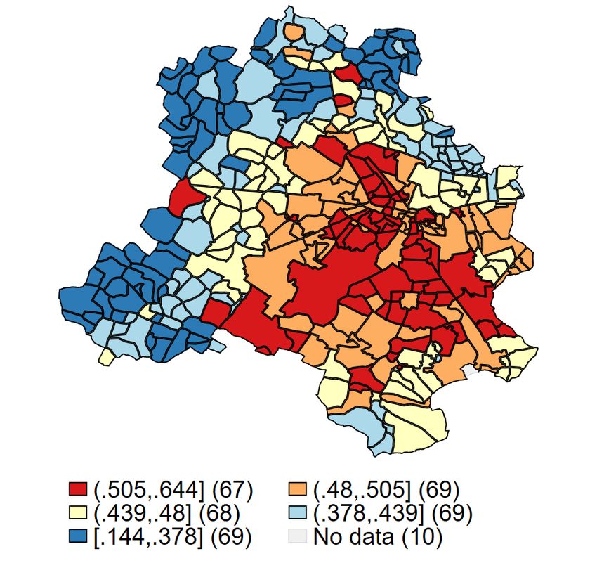
Use and dissemination of this working paper is encouraged; however, the JICA Research

Institute requests due acknowledgement and a copy of any publication for which this

working paper has provided input. The views expressed in this paper are those of the

author(s) and do not necessarily represent the official positions of either the JICA

Research Institute or JICA.

JICA Research Institute

10-5 Ichigaya Honmura-cho

Shinjuku-ku

Tokyo 162-8433 JAPAN

TEL: +81-3-3269-3374

FAX: +81-3-3269-2054
Heterogeneous Effects of Urban Public Transportation on

       Employment by Gender: Evidence from the Delhi Metro∗

                                   Mai Seki† and Eiji Yamada‡

Abstract
The Delhi Metro is one of the leading examples of a recent urban mass transit infrastructure
project in a developing country where women have traditionally suffered from constrained
mobility. In this paper, we analyze the effects of the Delhi Metro on the work participation
rate of women and men, using a three-period (1991, 2001, and 2011) panel data of township-
level zones within the city of Delhi. While the data has limitations in understanding the
characteristics of individual residents in detail, we employ a difference-in-differences
estimation controlling for a location fixed-effect, with a parallel trend test. The results
suggest that the proximity to the Delhi Metro stations significantly increases the female
work participation rate (WPR), whereas its effect on the male WPR is ambiguous with the
potential to have an opposite sign. While there are number of potential mechanisms that
can deliver this result, we develop a theoretical urban commuting model and argue that a
larger reduction in the commuting cost for females (by offering a safer commuting mode of
transportation, for example) can generate the quantified patterns of the effects on the WPR.
Overall, our results relate to the literature on the quantification of the contribution of urban
transport infrastructure towards inclusive growth and poverty reduction.

Keywords: India, gender gap, equilibrium commuting model

JEL: O18, J20, R00
   ∗
    This paper was prepared under a JICA-RI project titled "Study on the Methodology of Impact Analysis
for Infrastructure Projects". We are thankful to the seminar participants at Lisbon 2017, GRIPS 2017,
Niigata 2017, ISEC Bengaluru 2018, JEA Kobe 2019, and JASID Tokyo 2019. We are also grateful to Prof.
Takashi Kurosaki, Prof. Kensuke Teshima, and two anonymous reviewers for their valuable comments for
the earlier versions of this paper. The study was prepared by the authors in their own personal capacity.
The opinions expressed in this article are the authors’ own and do not reflect t he o fficial p ositions o f
either the JICA Research Institute or JICA. All errors are ours.
   †
     Ritsumeikan University (maiseki@fc.ritsumei.ac.jp)
   ‡
     JICA Research Institute (Yamada.Eiji@jica.go.jp)

                                                     1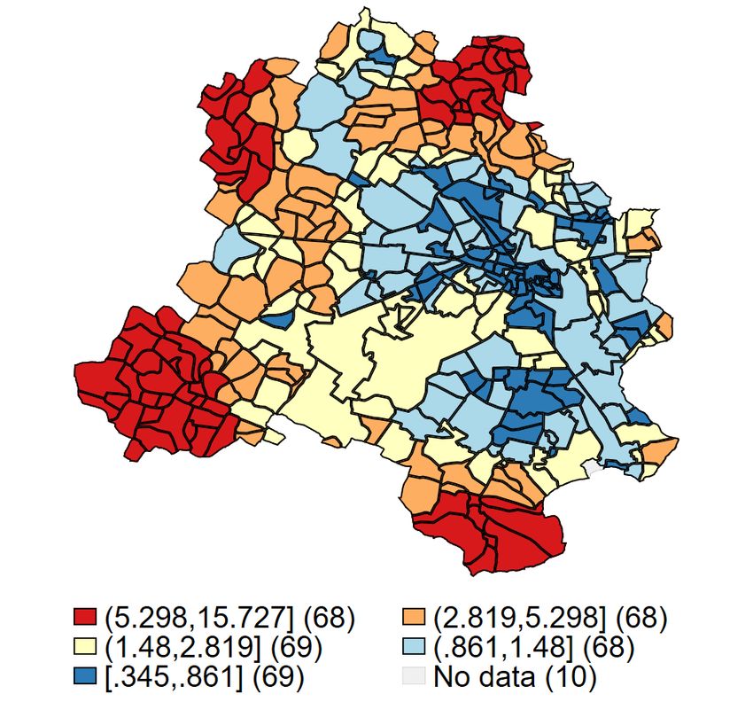
1. Introduction

In the past seventy years, the share of urban dwellers has steadily increased in developing
countries, and this trend will continue in the coming decades (United Natations 2019).

India is one of the main contributors to the global urban population growth, which is

projected to add 416 million urban residents by 2050. To mitigate traffic congestion ac-

companied by the continuing urbanization, many countries including India are investing in

urban public transportation systems. While the overall mobility of residents improves and
city production capacities expand, gender inequality of mobility in urban areas remains an

unresolved issue (Peters 2013; Uteng 2011; Hyodo et al. 2005). According to previous stud-

ies, women in the urban areas of the developing countries go out of home less frequently,

and depend more on public transportation than men. The provision of safe and accessible

public transportation could potentially improve female mobility, a necessary conditoin for

their further active participation in the economy.

    In fact, a gender mainstreaming in the infrastructure projects of developing countries

has gained attention from policy makers over the past decade (Asian Development Bank

2013; African Development Bank Group 2009; UN Women 2014; World Bank 2010). How-

ever, there is still only a limited amount of research quantifying the development impact,

especially on how women and men are differentially affected by urban transport develop-

ment.   1   There are studies that have discussed gender heterogeneity in commuting time to

work and its impact on labor supply (Gutiérrez-i-Puigarnau and Ommeren 2010; Gimenez-
nadal and Molina 2014; Gimenez-Nadal and Molina 2016; Zax 1991; Black, Kolesnikova,

and Taylor 2014); however, they do not necessarily focus on public transportations in a
   1. There is a large literature on the effect of subways on employment density in the developed countries
such as that by Redding and Turner (2015). However, very few impact evaluations of urban transportation
exist in the developing countries. Majority features rural roads and some major studies discuss inter-city
highways or railroads (Seki, 2016).

                                                    2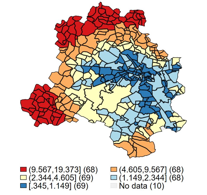
given country context, except the ones by Kawabata and Abe (2018) and Gaduh, Grac-

ner, and Rothenberg (2018). Kawabata and Abe (2018) analyze the commuting and labor

supply patterns of married couples, resident in the greater Tokyo metropolitan area using

GIS. Gaduh, Gracner, and Rothenberg (2018) estimate an equilibrium model of commuting

choices with endogenous commuting time to assess the impact of counterfactual transporta-

tion policies, using the data collected for the detailed urban transport plannings in Jakarta

before and after the Bus Rapid Transit (BRT) system was commissioned. Each of these

studies on gender-heterogeneous commuting time suggest the importance of examining the

heterogeneous impact of public transportation on employment by gender, rather than sim-

ply an overall effect. More closely related studies have documented the correlations between

the access to transportation and labor market outcomes such as income or employment in

developing countries (Hyodo et al. 2005; Goel and Tiwari 2016; Glick 1999). These studies

use cross-sectional data, so we decide to further extend this line of research by utilizing

panel data. A similar line of research using panel data from Lima, Peru on BRT and light

rail system is summarized in a working paper by Martínez et al. (2018). But the most

relevant analysis, which is ongoing, can be found in the field-experiments being conducted

in Lahore, Pakistan for assessing the impact of providing women-only-wagons (a safety

measure) to feed into a BRT system on female employment (Majid et al. 2018).2

   In this paper, we analyze the effects of the Delhi Metro, one of the largest mass rapid

transit systems in the current world that has been developed since the early 2000s, on

the work participation of women and men, to provide quantitative evidence on whether a

high quality urban public transportation system contributes to an improvement in female

economic participation. We focus on the Delhi Metro for three reasons. Firstly, Delhi is
   2. Majid et al. (2018) reports the effects of BRT on congestion, and a progress of the
RCT based impact analysis of safe commuting for female is available in the J-PAL’s website:
https://www.povertyactionlab.org/evaluation/impact-public-transport-labor-market-outcomes-pakistan

                                                3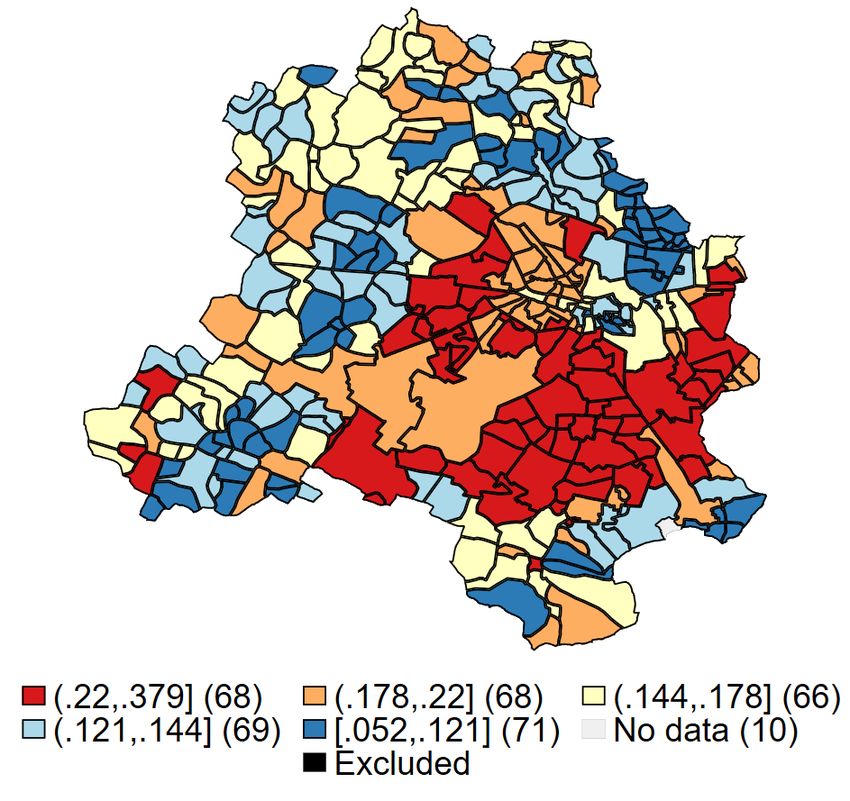
one of the cities in the world fighting a gainst s evere c oncerns f or f emale s afety i n public

spaces and transportations (Jogori and UN Women 2011; Safetipin 2016). According to a

Thomson Reuters Foundation Annual Poll in 2017, “New Delhi, the world’s second most

populous city with an estimated 26.5 million people, was ranked as the worst megacity

for sexual violence and harassment of women alongside Brazil’s Sao Paulo."3 Also, an UN

Women supported survey in Delhi shows that 95 percent of women and girls feel unsafe

in public spaces in their 2013 report. Even after the introduction of the Delhi Metro, the

situation is still severe but it was even worse before. Recent studies reveal that safety

matters to females that have choices in their lives. For example, Borker (2017) finds that

safety of school-commuting route has a direct impact on the university choice among the

female students in the city of Delhi. In her study, she finds that the willingness to pay for

women for a school-commuting route that is one standard deviation safer is an additional

18,800 rupees (290 USD) per year, relative to men, which is an amount equal to double

the average annual college tuition. Secondly, India faces challenges over female economic

participation and empowerment. Female non-agricultural labor participation has been

historically stagnant in South Asia, and there has even been a declining trend in India at

the national level (Klasen and Pieters 2015; Andres et al. 2017). For the city of Delhi,

while the labor participation of women has not declined, its growth has been stagnating

compared to that of men. Lastly, Delhi Metro is one of the best cases to analyze the

impact of high quality urban transport infrastructure in developing countries, given its

reputations for high service standards. This reputation is not only for its stability and

convenience, but also for the safety and comfortable travel of its female passengers. Based

on the interviews with users, the introduction of Delhi Metro is shown to have drastically

changed transportation choice for women, due to the high standard of safety in the Metro
  3. https://poll2017.trust.org/

                                                4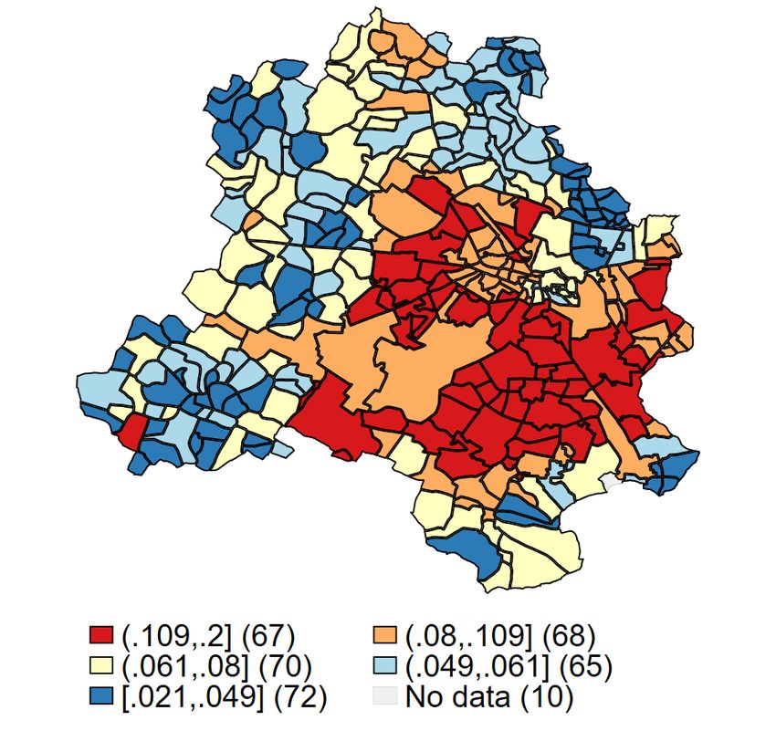
system (Takaki and Hayashi 2012; Onishi 2017). Motivated by these factors, the existence

of the female mobility issue, concerns for female labor supply, and a suitable treatment, we

hypothesize the introduction of a safe mode of public transportation in Delhi would have

had a non-negligible effect on the supply of female labor (the commuting-safety hypothesis),

along with other factors, such as residential relocation, compositional change in labour

demand and/or family-level joint labor supply decisions. In this study, we try to quantify

the gender-heterogeneous effects of the Delhi Metro system on work-participation rates as

the first step in our analysis, solely due to the data limitation.

   While our aim has a great policy relevance, it is a difficult research question to obtain

a rigorous quantitative answer on because of severe data limitations. First, the standard

identification concerns from the non-random location of physical infrastructure are in-

evitably applicable. This fundamental identification challenge cannot be resolved even if

there will be more detailed data available except when there is a suitable natural exper-

iment. Moreover, other impeding facts, like the lack of appropriate individual-level data

that covers the period before and after the commission of the Metro as well as the fact

that a long time has past since the initial commission of the Metro in 2002, keep us away

from making a rigorous causal arguments in an ideal empirical setting.

   Our strategy is therefore to use the best-available data and carefully argue its empirical

limitations. More specifically, we use the Primary Census Abstract (PCA) which provides

various tabulations from the Population Census data for finely disaggregated geographical

areas within the National Capital Territory (NCT) of Delhi. We construct a panel of PCA

zones for three consecutive census years, 1991, 2001, and 2011. As the measure of interven-

tion, we calculate an accessibility from each PCA zone to the nearest metro station, using

maps of PCA zones and the alignment of the Delhi Metro. With the calculated treatment

variable, proximity to the Delhi metro, we conduct a difference-in-differences (DID) analy-

                                              5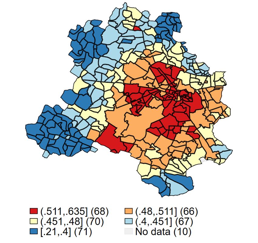
sis, controlling for location fixed effect (time-invariant unobserved heterogeneity), to assess

whether the proximity to metro stations contributes to the area’s growth in female and

male participation in non-agricultural economic activities. Since we construct these panel

data at the level of the PCA zone-level geographical unit for three rounds (1991, 2001, and

2011) with two pre-treatment periods, we can examine the parallel trend hypothesis which

is the prerequisite for DID, by including the “lead" term in the estimation equation.

   We find that the effect of the proximity to the Delhi Metro on female work participation

rate is positive, and that the same does not seem to hold for men (rather the opposite).

This is suggestive evidence that there could be a gender-heterogeneous impact from the

Delhi Metro system on the decision of economic participation. In other words, women

might respond more positively than men to the proximity to the Delhi Metro stations in

deciding whether or not to work.

   To understand these empirical findings, we develop a spatial model of urban trans-

portation and commuting. We explicitly model the commuting choice of female and male

urban residents who face different commuting costs (fees and travel time plus safety-related

welfare cost). We study the model’s comparative statics to see how a hypothetical Metro

project would affect female and male work participation rates across different zones in a

city. We find that if the Metro reduces female commuting costs more than men’s, female

WPR increases in zones closer to the Metro despite male WPR exhibiting a more ambigu-

ous (or opposite) relationship. This theoretical example shows consistent patterns with

our empirical results.

   Our empirical findings have a limitation, however, in that the rigorous causal identifi-

cation of the impact or investigation of a mechanism is affected by the nature and extent of

the available data. For example, the gender wage gap or gender-heterogenous comparative

advantage in specific skills may result in higher demand for female workers rather than male

                                              6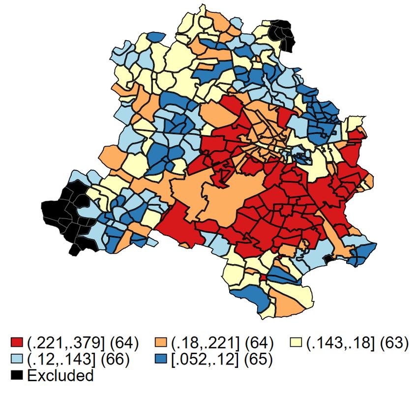
workers near the metro. However, we do not have gender-specific w age d ata o r skill-level
employment information by gender at such a fine g eographical u nit, s o t hese hypotheses
are currently unable to be separated from the commuting-safety hypothesis. Nevertheless,
our study is one of the first attempts to quantitatively measure the gendered implication of
a large scale urban public transport development in the context of megacities in developing
countries.
The rest of the paper is organized as follows. In Section 2, we briefly g o o ver the
background of the Delhi Metro project. Section 3 describes the data and Section 4 discusses
empirical specifications. S ection 5 r eports t he r esults. I n S ection 6 , w e d evelop a spatial
urban model that shows that the commuting-safety hypothesis has an equilibrium that is
consistent with our empirical findings. S ection 7 d iscusses t he l imitation o f o ur method
and potential directions for future research.
2. Background of Delhi Metro
As the country’s third urban mass rapid transit system (MRT) and the first of its kind in
the capital city, the Delhi metro project has been developed over the past seventeen years.
The first phase of Delhi Metro project consisted of the 58 stations and lines covering 65km
and commissioned during 2002-2006. Following the Phase I, Phase II built 85 stations and
lines covering 125km, which were commissioned during 2008-2011. As of the end of 2011,
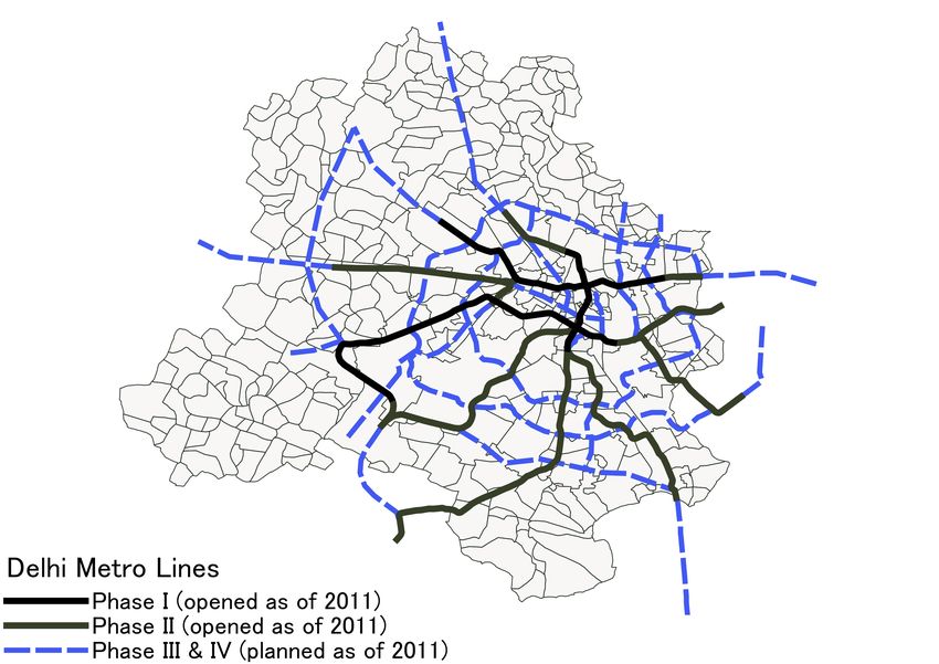
Phase III and Phase IV were in the planning stage. The geographical alignments of the Delhi
Metro lines in the different phases are shown in Figure 1.
The novelty of the Delhi Metro project is the fact that it focused on the safety and
inclusiveness from its planning stage. Adaptation of women-only car, barrier-free design,
rubbish control for keeping train clean, and security check at the entry have contributed
towards providing safe public mass urban transportation for the citizens of Delhi. Overall,
7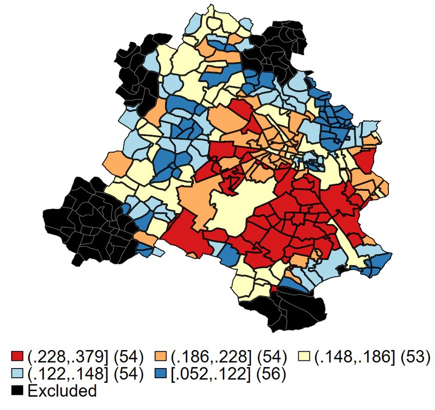
the Delhi Metro has gained a reputation for high standard of facility and operation that

ensures safety and comfort for female passengers (Takaki and Hayashi 2012; Onishi 2017).

   Prior to the introduction of the Delhi Metro, safety concerns in the public transporta-

tion system had been severe for women in Delhi (Jogori and UN Women 2011; Safetipin

2016). While affordable and reliable urban transportation plays a vital role in engaging in

either income-generating activities and schooling in optimal locations, or other activities

such as household chores, family visits, or leisure, it is not difficult to hypothesize that the

limitation of safe modes of transportation was taxing for women in trying to get access to

these social and economic opportunities. Given such a context, the introduction of a rela-

tively safe public transportation system has had a potential impact to drastically change

women’s behavior in Delhi.

                              Figure 1: Delhi Metro Alignment

   Source: The authors construct this map based on GIS maps procured from the following GIS map
 vendors. Base-map with zone boundaries: Zenrin Co., Ltd. Metro Alignment: Compare Infobase Ltd.

                                                8
3. Data
We use the Primary Census Abstract (PCA) of India’s Population Census in 1991, 2001,
and 2011, published by the Office of the Registrar General and Census Commissioner,
Ministry of Home Affairs. The PCA provides aggregates of population census enumeration
at the level of a small local administrative unit and/or a ward of constituency. In 1991, entire
area of the NCT of Delhi was divided into towns, villages, and charges.4 Since the
geographical boundaries of administrative units change overtime, we interpolate the data
of 2001 and 2011 based on area size so that the boundary is consistent with that of 1991.
We carry out spatial interpolation as follows. To simplify the explanation, we consider
the case of two period, period 0 and period 1. Suppose there are a total of J0 zones in
the period 0, indexed as j0 = 1, ..., J0. In period 1, suppose there are a total of K1 zones
indexed as k1 = 1, ..., K1. The boundaries of zones are not in general consistent between
the two periods, which means that a zone in period 0 intersects with multiple zones in
period 1. Consider a particular zone j0 of the period 0 which intersects with multiple
period 1 zones. Let Sj10 denote the set of these period 1 zones intersecting with j0. For
each of these period 1 zones k1 ∈ Sj10 , the area can be divided into a part intersecting with
j0 , denoted as ajk01 , and the remaining part, a−j0
k1 which does not intersect with j0 . Our
spatial interpolation calculates the period 1 value of zone j0 statistics by taking a weighted
average of the statistics of the intersecting period 1 zones in Sj10 . More specifically, the
interpolated value of variable x for zone j0 in period 1 is given by:
X ajk01
x̃1j0 = xk1 (1)
k1 ∈Sj1
ajk01 + a−j
k1
0
0
4. Charge is an electorate unit which disintegrated the central part of Delhi in the 1991 Census. In the
1991 Census, disaggregated data for the MCD (Municipal Corporation of Delhi), consisting the central part
of the NCT of Delhi, were reported at the level of Charge.
9This interpolation only applies to the variables in levels, such as population and the number
of workers. For the variables in rates, we calculate them using the interpolated level
variables. For example, a rate variable r which is defined as the ratio of two level variables
ỹj1
x and y, or r = xy , we obtain the period 1 interpolated value by r̃j10 = 0
x̃1j
. To check the
0
robustness of the key results of this interpolation, we add the analyses using only those
zones with consistent boundaries over time in Section C of the appendix.
To represent the economic participation of each gender group from the available statis-
tics, we calculate “(non-agricultural) work participation rate” (“WPR” hereafter). The
work participation rate is measured by the ratio of the number of “main workers” (works
more than 6 months per year) in “other sectors”(other than cultivators, agricultural labour-
ers, or household industry workers)5 divided by the adult population6 , for each gender. This
indicator is different from the labor force participation rate (LFPR). While the denomina-
tor of LFPR is usually the working-age population above the age of 15, the denominator of
WPR is the (imputed) adult population. Moreover, the numerator is also different because
the definition of being a labor force includes those who are employed and unemployed,
while that of work participation rate does not include those who are seeking for a job.
These definitional differences make WPR either smaller or larger than LFPR, which is
an empirical question because the difference in the denominators depends on how all-ages
population minus two times the 0-6 population differs from the population over 15. In
fact, the urban areas’ LFPR during these periods has increased from 14.7 percent to 15.5
5. The “Other Sector”: All workers, i.e., those who have been engaged in some economic activity during
the last one year, but are not cultivators or agricultural labourers or in the Household Industry, are ’Other
Workers(OW)’. The type of workers that come under this category of ’OW’ include all government servants,
municipal employees, teachers, factory workers, plantation workers, those engaged in trade, commerce,
business, transport banking, mining, construction, political or social work, priests, entertainment artists,
etc. In effect, all those workers other than cultivators or agricultural labourers or household industry
workers, are “Other Workers”.
6. Since the adult population is not given in PCA, we impute it by “total population - 2 x (population
of 0 to 6 ages)”, base on the population pyramid of India.
10percent, while Delhi’s WPR increased from 7.06 percent to 7.91 percent. Though the lev-
els are different due to the definitional difference discussed above, the trend is consistent
across the two measures.
Our treatment variable is the proximity of a zone (a town, a village, or a charge based
on the 1991 administrative boundaries) to its nearest Metro Phase I and II stations. To
represent the proximity to Metro stations, we measure the average distance using the
coordinates of boundaries of towns and villages, as well as the alignment of the Metro
stations. The average distance measure is constructed as follows: (i) A large number of
equally spaced points (about 0.5 million) are generated and plotted over the entire area of
Delhi; (ii) From each point, the nearest Metro station is searched and the distance from the
point to the nearest Metro station is calculated. For a point k located within the boundary
of zone i, this distance is denoted as dk(i) ; and (iii) The average distance to the nearest
Metro station(s) of the zone i, Di , is then calculated as
P
k(i) dk(i)
Di = (2)
Ni
where, Ni is the number of points in zone i. Di is smaller (i.e. the treatment inten-
sity is larger) if i is closely located to Metro stations opened during 2002-2011, after the
commission of the Phase I and II Metro network. Average distance measures to the the
Metro Phase III and IV (only under the planning phase in 2011) are also calculated in
the same manner to better define the comparison group that is more likely to share the
similar unobserved characteristics regardless of the assigned treatment. In addition, we
use the total population, the number of children, the number of households, the number
of literal residents, and the number of residents scheduled caste (each by gender) from the
PCA tables as control variables in the main analysis (the analysis without these controls
11are available in the robustness check).7
The descriptive statistics is shown in the Table 1. The upper table summarises our
time-invariant variables, and the lower one is for time-variant variables. Our time-invariant
variables are the distances to the Phase I and II metro stations that had commissioned by
2011, and those of the Phase III and IV which had not yet opened. On average, distance
to the nearest Phase I or Phase II metro station is 5.2 km. Since the location of the
planned metro stations, those of Phase III and IV, are more stretched out to the suburbs,
the average distance to the Metro station is shorter 3.3km.
The time-variant variables are the outcome variables and control variables used in the
estimation. Female WPR has been substantially lower than that of males throughout two
decades since 1991. However, their average WPR has increased from 5.3 percent in 1991
to 7.9 percent in 2011, while men’s WPR has grown from 40.4% to 45.3% during the same
period. In contrast to the national level decline in labor force participation of women, the
small increase of their WPR in Delhi might be partially due to the contribution of the
Delhi Metro.
Figure 2 depicts kernel density estimates for the distribution of female and male WPRs
for years 1991, 2001, and 2011. First, we can observe that the WPR distributions are
distinctly different between the two gender groups in each year. That of females are
clustered at lower rate of WPR with smaller variance, in contrast to that of males. Secondly,
there is a subtle, but universal shifts of female WPR distribution towards the right. This
suggests that the rate was improving almost everywhere in the distribution for women.
Male WPR initially had a flat distribution in 1991 while it had evolved into a single
peaked one in 2001. We do not observe a distinct shift in the distribution from 2001 to
7. Under the constitution of India, scheduled caste is defined as follows. http://socialjustice.nic.
in/writereaddata/UploadFile/Compendium-2016.pdf. India’s Census follows this definition. See http:
//censusindia.gov.in/Census_And_You/scheduled_castes_and_sceduled_tribes.aspx.
122011.8
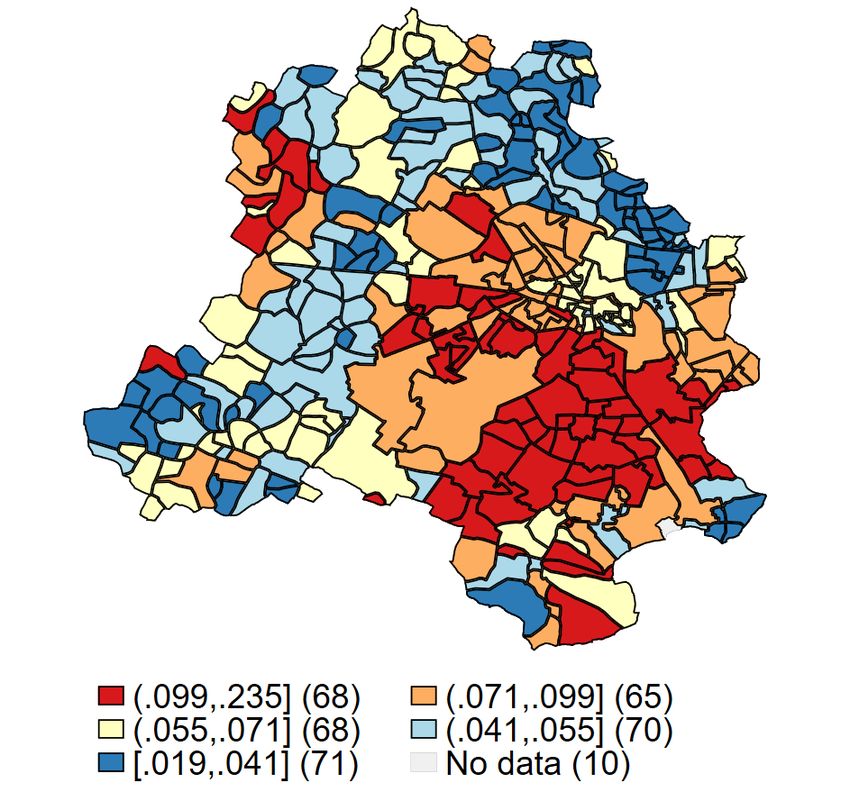
Figure 3 shows the spatial distribution of WPR of females and males for the two census
years, 2001 and 2011. The dark-red zones are places with the highest WPR and the dark-
blue zones are with the lowest WPR. The top two panels, 3a and 3b show women’s WPR.
The bottom two, 3c and 3d are those for men.
Table 1: Summary Statistics
(1) (2) (3)
Time-invariant variables N mean sd
Dist. to Phae I or II Metro St. (km) 342 5.239 4.763
Dist. to Phae III or IV Metro St. (km, used for 342 3.274 3.145
sub-sample selection)
1991 2001 2011
(1) (2) (3) (4) (5) (6) (7) (8) (9)
Time-variant variables N mean sd N mean sd N mean sd
Female WPR 332 0.0531 0.0599 342 0.0706 0.0369 342 0.0791 0.0371
Male WPR 332 0.404 0.131 342 0.439 0.0812 342 0.453 0.0674
Female to male WPR ratio 332 0.118 0.0993 342 0.161 0.0864 342 0.171 0.0644
Household Size 332 5.562 0.982 342 5.283 0.478 342 5.038 0.396
Children Share 332 0.184 0.0369 342 0.150 0.0235 342 0.124 0.0171
Female to male literacy ratio 332 0.698 0.163 342 0.817 0.0679 342 0.865 0.0485
Female to male SC ratio 327 1.007 0.155 342 1.042 0.0574 342 1.027 0.0362
Note: The upper table summarizes the time-invariant variables. The lower one is for the time-
variant variables.
8. The T-test comparing the means of WPR across different years show that the mean WPR has signifi-
cantly increased over time for both genders. We also conduct the Kormogolov-Smirnov test to statistically
assess whether the WPR distribution changes across years. The results indicate that women’s WPR has
different distribution across three census years, while the men’s distribution between 2001 and 2011 are not
statistically distinguishable. The results are reported in Table A.1 in the Appendix.
13Figure 2: Kernel Distribution of Female and Male WPR, 2001 and 2011
Source: Authors
14Figure 3: Spatial Distribution of WPR for females and males, in 2001 and 2011
(a) 2001 Female WPR (b) 2011 Female WPR
(c) 2001 Male WPR (d) 2011 Male WPR
Source: Authors
15Figure 4: Distance to Commissioned and Planned Metro Stations
(a) Distance to Commissioned (PH I & II) (b) Distance to Planned (PH III & IV)
Metro Stations Metro Stations
Source: Authors
164. Empirical Strategy
As described in Section 3, our data is neither experimental nor quasi-experimental. The
unit of observation is aggregated at the level of zones (town or ward), which divide the
NCT (National Capital Territory) of Delhi into 342 geographical units. Using a panel
data of zones in Delhi for 1991, 2001 and 2011, we employ the difference-in-difference
(DID) method with two pre-treatment periods (1991, 2001). In estimation, we check for
parallel pre-trend by exploiting these two pre-treatment periods. Specifically, we estimate
the following equation:
Yit = β0 + β−1 (Di × P ret ) + β(Di × P ostt ) + δXit + θt + αi + it , (3)
Where, Yit is the outcome variable of zone i at year t; Di is the treatment variable, the log
of average distance to nearest Phase I or II metro station, P ret is a time dummy taking
1 when t = 1991 and 0 otherwise. P ostt is another time dummy taking 1 if t = 2011 and
0 otherwise. Coefficient β is our central interest. This is the post-treatment effect of the
distance to the metro station on the outcome. β−1 captures the correlation between a zone’s
distance to the metro station and the outcome variables in 1991. If β−1 is insignificant, we
will not reject the hypothesis that pre-trend is not associated with the distance to a metro
station, suggesting that the parallel pre-trend hypothesis holds. The same strategy has
been used in studies such as Autor (2003) and Kearney and Levine (2015). Xit is a vector
including other time-variant location specific characteristics such as average household size,
share of children (under 6 years old) in the population, female literacy rate relative to male,
17and ratio of share of scheduled caste between female and male.9 The first two variables are
introduced to control for the variations in the presence of dependents in household (i.e.
elderly and children) which are not directly measured in the PCA. The latter two control
for the variation in the gender inequality.10 Lastly, θt is year fixed effect, α i is a zone-level
fixed e ffect, a nd it i s t he e rror term.
The goal of this paper is to empirically assess how the Delhi Metro differently affects
the economic participation of women and men. More specifically, w e i nvestigate whether
the zones closer to the Delhi Metro station have observed more increase in work partici-
pation of the residents than those in zones further away from metro stations, separately
for women and men. In the empirical analyses below, we focus on four measures of work
participation, female WPR, male WPR, a ratio of a zone’s female WPR to male WPR
(= W P R(women)/W P R(men)), or “WPR ratio” in short; and WPR for total residents
(sum of females and males).
For the treatment variable, Dj , we define the (log) distance to the nearest Phase I or II
Delhi Metro station. The reason for this choice of continuous treatment variable is twofold.
Firstly, we would like to avoid a discretionary construction of a treatment variable, which
is unavoidable when using discrete variables (i.e., we do not know from which kilometer it
is “proximate” to the metro). Secondly, it is rather easier to interpret the results.
We estimate this equation 3 with a standard fixed e ffects e stimator. T he coefficient
β will capture the treatment effect, and the sign and the magnitude of this coefficient is
our central concern. β−1 is the coefficient on the “lead” term. We expect that β−1 is
insignificant u nder t he c ommon t rend a ssumption. P lease n ote t hat t he i nsignificance of
Population
9. For clarity, variables are given by; average household size = Number of Household
; share of chil-
Number of Children (under 6)
dren (under 6 years old) in the population = Population
; female literacy rate rela-
female literacy rate
tive to male = male literacy rate ; and ratio of share of scheduled caste between female and male =
share of scheduled caste in female population
share of scheduled caste in male population
10. In the separate regression, we check that these variables do not seem to be the consequences of the
treatment Di × P ostt , allowing us to included them as controls in the equation.
18β−1 , is only suggestive evidence that the two sets of zones (in this case near and far from
the new metro stations) would have evolved similarly in the absence of the intervention. It
is not decisive as to whether there is unobserved heterogeneity across regions affecting the
change in outcome variables or not. In fact, recent studies such as Kahn-Lang and Lang
(2019) as well as Jaeger, Joyce, and Kaestner (2018) note that the parallel pre-trends do
not necessarily imply parallel trends.
We conducted the estimation across various sub-samples to see how the results are
sensitive to the selection of the comparison group. We compare five sub-sample defined as
follows; (1) All the zones in Delhi (Figure 5a); (2) includes only the zones within 10km
reach from the nearest commissioned (Phase I or II) station or the nearest planned (Phase
III or IV) Metro station (Figure 5b); (3) includes only the zones within 5km reach from
the nearest commissioned (Phase I or II) station or the nearest planned (Phase III or IV)
Metro station (Figure 5c); (4) trims the zones in the subset (2) so that it include only
zones at least 10km further from the CBD of Delhi, Connaught Place (Figure 5d); and (5)
trims the zones in the subset (3) so that it include only zones at least 10km further from
the CBD of Delhi, Connaught Place (Figure 5e).
19Figure 5: Subsample Definition and “WPR ratio” in 2011
(b) Within 10km reach from commissioned and
(a) All zones in Delhi (1)
planned Metro Stations (2)
(d) Within 10km reach from commissioned and
(c) Within 5km reach from commissioned and
planned Metro Stations and at least 10km further
planned Metro Stations (3)
from the CBD (4)
(e) Within 5km reach from commissioned and
planned Metro Stations and at least 10km further
from the CBD (5)
Source: Authors
205. Results
Tables 2-5, report the results of the estimations across different specifications. Table 2
reports the estimation results of equation (3) taking the female WPR as the outcome.
For all the five s ubset a nalyses, o ur t reatment variable, D it , i s s ignificant at th e 1 percent
significance l evel w ith n egative s ings, e xcept f or c olumn ( 5) w here s ignificance is at th e 5
percent significance l evel. N egative c oefficient i ndicates t hat b eing c lose t o t he commis-
sioned Metro station makes female work participation rate higher. For example, for the
full sample case, shown in column (1) of the Table 2, if the distance to the nearest Phase
I or II station becomes doubles, female WPR decreases by 0.558 percentage points. Given
that the mean of female WPR in 2011 was 7.91 percent, this implies that doubling the
distance around the mean distance of 5.239km will reduce WPR of females to 7.35 percent.
Columns (2) and column (3) of Table 2 limit the sample zones to within 10km and 5km
access to any Metro station regardless of whether they had already been commissioned as
of 2011 (i.e., "control group" is restricted to the areas near Phase III or IV). We regard that
the zones closer to the planned network are “selected” for Delhi Metro intervention, but
the metro service is not yet available at that point in time, so they may share the similar
unobserved heterogeneity with zones close to the commissioned stations, which affect the
change in outcomes.11 By estimating the model of columns (2) and (3), we compare the
outcomes in zones for those who got access to metro stations earlier with those who would
get it later. Therefore, by estimating the model only in those areas close to either the
commissioned or planned metro stations, we compare outcomes in zones between the areas
gaining access to the metro stations earlier (before 2011) and those would gain access later
11. To identify the causal impact of transport system, it is common to use planned but never developed
routes as control group; however, there is no such locations in Delhi Metro’s case. Instead, we adopt an
idea close to the phase-in approach for improving our identification. T he p hase-in a pproach i n o ur context
(or in transportation infrastructure projects in general) still suffers from the remaining endogeneity bias
due to the non-random construction timing/order of projects.
21(post 2011).
We also note that the effect seems to be stronger outside the central area. The mag-
nitude of the coefficient is greater for column (4), the outer area subsample, than that of
column (2) (the cut-off at 10 km). The same argument applies to the comparison between
columns (3) and (5), where the cut-off is 5km.
The results shown in the Table 2 suggest that a positive effect of the accessibility to
the Delhi Metro for females exists throughout all the specifications. Furthermore, for all
columns, the coefficients on the “lead” term are insignificant, which means that the common
pre-trend assumption holds for these sets of analyses.
Table 3 shows the results for the effects on male WPR. Contrary to the case for fe-
males, all the coefficients on the distance to a commissioned Metro station are positive
and significant at the 1 or 5 percent significance level. The parallel pre-treatment trend
assumption is overall satisfied except for column (3) whose coefficient β−1 term is negative
and statistically significant at the 10 percent level. Furthermore, the magnitude of the
effect does not vary across subsamples, ranging from 0.00801 to 0.00975, compared to the
case for females as shown in Table 2. From the results in Table 2 and Table 3, it turns
out that the proximity to the Delhi Metro station affects positively for female WPR while
its effects is negative for that of male. Given that the mean of WPR for males in 2011 is
45.3%, this implies that doubling the distance around the mean distance of 5.239km will
increase the WPR of males to 46.2%.
Table 4 reports the results when the outcome variable is the WPR ratio between female
and male. Consistent with the results in Table 2 and Table 3, the coefficients on the distance
to commissioned station are negative and significant at the 1 percent level. The results
implies that the gap of WPR between females and males becomes slightly smaller (i.e.
WPR ratio increases) in zones closer to commissioned Metro station. The key identifying
22assumption is again the common trend, and it seems to be satisfied for the trend between
1991 and 2001 as the coefficient β−1 is insignificant.
Finally, Table 5 reports the results when the total WPR is used as the outcome. Total
WPR is the sum of female and male main workers in the non-agricultural sector divided by
total adult population. For the first three columns show significantly positive coefficients
on the distance to the nearest commissioned Metro station, meaning that proximity to
a Metro station has a negative effect on total work participation. However, as shown in
columns (4) and (5), the effect becomes no longer significant in suburban subsamples. This
is mainly due to the imprecision in smaller sample sizes as the point estimates do not change
in magnitude comparing to columns (1)-(3), whiles the standard errors are larger. In the
area outside of the CBD premises, proximity to the Metro does not change the overall work
participation.
We add several robustness checks to address a series of technical concerns. The first
relates to the control variables we included in the estimation equation. If the control
variables are endogenous to the treatment variable, the inclusion of the controls in the
equation is problematic (Angrist and Pischke 2009). Therefore, we conduct the same
estimations without the control variables, as reported in Tables B.2-B.5 of Section B of
the Appendix. For women, the results are qualitatively the same as our main estimation.
For men, we have qualitatively similar results for our variable of interest (“Dist. to Metro
(2011)") without control variables compared with the case of our main model reported in
Table 3. However, the β−1 term becomes highly significant in this case. This implies that
the control variables we include in the main analyses capture the pre-trend heterogeneity
for the case of male WPR well.
We also check the sensitivity of the results against our method of interpolating the data
so that the boundary definition of the “zones" would be consistent with that of 1991. In
23Appendix C, we introduce an illustrative explanation of our interpolation method and its
potential effects on the statistical outcomes. We also report the estimation results only
using the data of zones with consistent boundaries. Again, the female results are stable,
while the male ones are sensitive to the choice of sample zones.
From the empirical findings above, we can summarize the effects of the Delhi Metro on
the work participation as follows. Firstly, female WPR in 2011 is higher in zones close to
the Delhi Metro station, while it is lower in the more distant zones whereas male WPR
is instead higher in these zones. From the results of robustness checks, estimating the
equation without controls and using only the 1991-boundary consistent subsample, we find
that the results for male WPR are sensitive to the settings while female ones are stable
overall. Therefore, it is safe to conclude that in the areas closer to Metro, the economic
participation of women expanded more intensively than that of men. Secondly, for women,
the magnitude of the effects is larger in the suburban subsamples. This means that the
heterogeneous responses by gender caused by the access to the Delhi Metro might be more
pronounced in the suburban area than in the CBD. Thirdly, partially reflecting the fact
that women are positively affected by proximity and men are negatively affected, the total
WPR is negatively affected, because the effects on men surpass those on women. The
last point suggests that it is important to separately analyze the effects of transportation
between females and males without averaging out the overall effects.
What is the mechanism that delivers this gender differentiated outcomes? One potential
story could be an additional mobility benefit that the Delhi Metro may provide for women.
The Delhi Metro is a mass rapid transit system which did not exist before in that city,
where road vehicles such as buses, three-wheelers, and rickshaws, are the major mode of the
transportation. The Delhi Metro has given citizens a faster and more reliable (predictable)
method for travel in the city. The time-saving effect of the Metro system contributes to
24a reduction of the travel cost of both males and females who use the system. Before the
introduction of the Metro, it is a plausible conjecture that female mobility was substantially
more constrained than men, considering the safety issues including sexual violence on public
transport. If the Delhi Metro secures a mode that allows females to travel more safely than
on other traditional modes, the effective travel cost for might be reduced by more than
just the time-saving effect. If this additional benefit is large, then whether to live in the
neighbourhood of the Metro station should matters more to the mobility of females than to
that of males. To argue this implication more formally, Section 6 introduces a theoretical
model that explains this potential mechanism.
Other than that, there are a couple of other mechanisms that could generate gender-
heterogeneous effects. Firstly, labor demand might change by the introduction of the
Metro and that could be gender-heterogenous. For example, the manufacturing sector
might relocate its factories and offices outside of the downtown core, while service sector
jobs might flourish downtown. Each sector might attract workers of a different gender.
One possibility is that males are mainly in manufacturing, and this causes their residences
to move further away from the metro, which is rather concentrated near the downtown
core, as the factories relocate to the suburbs. An alternative possibility is that women
tend to take job openings in service sector, and residents near the metro start working
as it stimulates demand for service sector jobs. Secondly, a reduction of congestion and
travel time that can plausibly benefit both females and males but in different magnitudes,
encourages the residents to commute further. Nevertheless, it also induces in-migration of
workers into areas near the Metro stations, and this results in higher work participation
rates and housing prices in those areas.12 The resulting residential relocation itself is hard
12. How WPR and housing price react also depends on the elasticity of housing supply, the spatial allo-
cation of industries within cities, and wage and many other things, making the actual signs and magnitude
of the impact ambiguous.
25to analyze due to the data limitations, but the imapct through this channel could be gender-
heterogenous as well. Thirdly, it is also important to note that the family level decision
process can complicate male and female labor supply decisions. For example, if a family
(couple) faces a reduction of travel time by the Metro and a high paid job becomes available
to the husband, one of the possible responses is the wife’s withdrawal from labor market
activity (increase home production), substituting for this an increase in the male labor
supply (i.e., intensification of division of labor). When all of these effects are combined, it
is possible that the family with a male-bread winner moved away from the metro into more
reasonably priced residential areas and his wife resigns job or does not seek employment.
This story, however, cannot fully explain a subtle but statistically significant gain in female
WPR closer to the metro stations, so we still think our safe-commuting hypothesis will
survive the further tests in future research. The remaining challenge would be to separately
identify the safe-commuting hypothesis versus gender-heterogeneous shifts in labor demand
(with crowd-out and/or location segregation by industry-gender combination) because both
stories can explain the current empirical findings on females.
26Table 2: Effects of Proximity to the Delhi Metro on the Female Work Participation Rate
(Difference-in-Differences)
(1) (2) (3) (4) (5)
ALL d < 10km d < 5km d < 10km d < 5km
VARIABLES & CBD > 10km & CBD > 10km
Dist. to Metro(2011, β) -0.00558*** -0.00688*** -0.00418*** -0.00906*** -0.00453**
(0.00146) (0.00166) (0.00152) (0.00230) (0.00207)
Dist. to Metro(1991, β−1 ) 0.00186 0.00173 0.00505 0.00152 0.00479
(0.00316) (0.00355) (0.00376) (0.00362) (0.00430)
Household Size -0.0855*** -0.0852** -0.0810** -0.0898* -0.0797*
(0.0317) (0.0344) (0.0317) (0.0463) (0.0439)
Children Share -0.124*** -0.131*** -0.136*** -0.113*** -0.129***
(0.0215) (0.0226) (0.0256) (0.0222) (0.0263)
Female to male literacy ratio -0.0923** -0.0938** -0.0589 -0.123*** -0.0911**
(0.0396) (0.0397) (0.0419) (0.0330) (0.0376)
Female to male SC ratio -0.0629*** -0.0727*** -0.0454* -0.0831*** -0.0553*
(0.0214) (0.0256) (0.0261) (0.0295) (0.0295)
Constant -0.0402 -0.0519 -0.0636 -0.0192 -0.0593
(0.0650) (0.0690) (0.0758) (0.0739) (0.0804)
Year Dummy YES YES YES YES YES
Observations 1,006 948 801 654 507
R-squared 0.443 0.449 0.431 0.529 0.470
Number of id 342 322 271 224 173
Adj-R 0.438 0.444 0.426 0.523 0.462
Note: Standard errors are clustered at the individual zone
*** pTable 3: Effects of Proximity to the Delhi Metro on the Male Work Participation Rate
(Difference-in-Differences)
(1) (2) (3) (4) (5)
ALL d < 10km d < 5km d < 10km d < 5km
VARIABLES & CBD > 10km & CBD > 10km
Dist. to Metro(2011, β) 0.00862*** 0.00993*** 0.00975*** 0.00801** 0.00829**
(0.00217) (0.00225) (0.00237) (0.00327) (0.00329)
Dist. to Metro(1991, β−1 ) -0.00638 -0.00829 -0.0102* 0.00160 -0.00281
(0.00493) (0.00525) (0.00609) (0.00428) (0.00485)
Household Size -0.347*** -0.332*** -0.334*** -0.360*** -0.359***
(0.0334) (0.0333) (0.0330) (0.0404) (0.0410)
Children Share -0.0362 -0.0432 -0.0719* -0.00120 -0.0471
(0.0412) (0.0427) (0.0368) (0.0460) (0.0308)
Female to male literacy ratio 0.0268 0.0191 0.0522 -0.0329 -0.0140
(0.0525) (0.0522) (0.0649) (0.0202) (0.0263)
Female to male SC ratio 0.0353 0.0163 0.0451 0.0510 0.0742
(0.0433) (0.0450) (0.0477) (0.0460) (0.0506)
Constant 0.951*** 0.918*** 0.883*** 1.011*** 0.943***
(0.103) (0.104) (0.0986) (0.106) (0.0808)
Year Dummy YES YES YES YES YES
Observations 1,006 948 801 654 507
R-squared 0.462 0.456 0.455 0.609 0.600
Number of id 342 322 271 224 173
Adj-R 0.457 0.451 0.449 0.604 0.594
Note: Standard errors are clustered at the individual zone
*** pTable 4: Effects of Proximity to the Delhi Metro on a ratio of the Work Participation Rate
of Females over that of Males (Difference-in-Differences)
(1) (2) (3) (4) (5)
ALL d < 10km d < 5km d < 10km d < 5km
VARIABLES & CBD > 10km & CBD > 10km
Dist. to Metro(2011, β) -0.0166*** -0.0210*** -0.0120*** -0.0278*** -0.0160***
(0.00438) (0.00476) (0.00395) (0.00676) (0.00542)
Dist. to Metro(1991, β−1 ) 0.000604 0.00132 0.0120 -0.00377 0.0101
(0.00674) (0.00748) (0.00760) (0.00919) (0.00969)
Household Size -0.138** -0.145** -0.131** -0.164** -0.134*
(0.0556) (0.0598) (0.0546) (0.0809) (0.0753)
Children Share -0.265*** -0.279*** -0.230*** -0.280*** -0.219***
(0.0412) (0.0411) (0.0410) (0.0532) (0.0459)
Female to male literacy ratio -0.130** -0.128** -0.0700 -0.172*** -0.117**
(0.0567) (0.0569) (0.0614) (0.0466) (0.0541)
Female to male SC ratio -0.153** -0.131** -0.0770* -0.164** -0.0952*
(0.0614) (0.0563) (0.0460) (0.0730) (0.0539)
Constant -0.136 -0.151 -0.0805 -0.120 -0.0575
(0.117) (0.120) (0.120) (0.149) (0.135)
Year Dummy YES YES YES YES YES
Observations 1,006 948 801 654 507
R-squared 0.348 0.361 0.387 0.379 0.365
Number of id 342 322 271 224 173
Adj-R 0.343 0.356 0.381 0.372 0.355
Note: Standard errors are clustered at the individual zone
*** pTable 5: Effects of Proximity to the Delhi Metro on the Work Participation Rate of the
Sum of Females and Males (Difference-in-Differences)
(1) (2) (3) (4) (5)
ALL d < 10km d < 5km d < 10km d < 5km
VARIABLES & CBD > 10km & CBD > 10km
Dist. to Metro(2011, β) 0.00326** 0.00326** 0.00406** 0.00131 0.00289
(0.00152) (0.00163) (0.00160) (0.00233) (0.00218)
Dist. to Metro(1991, β−1 ) -0.00233 -0.00328 -0.00299 0.00170 0.000285
(0.00381) (0.00419) (0.00475) (0.00321) (0.00364)
Household Size -0.254*** -0.248*** -0.249*** -0.266*** -0.263***
(0.0264) (0.0278) (0.0261) (0.0359) (0.0351)
Children Share -0.0787*** -0.0859*** -0.103*** -0.0578* -0.0900***
(0.0295) (0.0309) (0.0284) (0.0317) (0.0232)
Female to male literacy ratio -0.0296 -0.0339 -0.000773 -0.0773*** -0.0543**
(0.0444) (0.0443) (0.0518) (0.0210) (0.0229)
Female to male SC ratio 0.0118 0.00323 0.0314 0.0116 0.0355
(0.0295) (0.0296) (0.0315) (0.0281) (0.0297)
Constant 0.539*** 0.519*** 0.499*** 0.582*** 0.531***
(0.0757) (0.0785) (0.0778) (0.0779) (0.0648)
Year Dummy YES YES YES YES YES
Observations 1,006 948 801 654 507
R-squared 0.474 0.466 0.467 0.642 0.634
Number of id 342 322 271 224 173
Adj-R 0.469 0.461 0.461 0.638 0.629
Note: Standard errors are clustered at the individual zone
*** p6. Theoretical Explanation with a Spatial Commuting Model
The empirical results indicate that the commission of the Delhi Metro raises the work
participation rate of women living nearby the Metro stations, while its effect is ambiguous
for men (this is the opposite of women in our main specification, b ut i t i s h ighly sensitive
to the inclusion of control variables).
In what follows, we try to argue that the observed results in WPR for women and men
can be caused by the heterogeneous reduction of commuting cost by gender, owing to the
Metro. Here, the commuting cost includes not only fees and opportunity cost, but also a
safety-related welfare cost. Especially, using a simple theoretical model of urban spatial
economy, we find t hat w omen’s W PR i s p ositively a ssociated w ith p roximity t o t he Metro
while men’s response is opposite (or ambiguous), if the reduction of commuting cost by
the metro is much larger for women than men.
Our theoretical model basically follows the modelling strategy by Ahlfeldt et al. (2015)
and Monte, Redding, and Rossi-Hansberg (2018), who study the residence-commuting
choice of households within an urban area. Like their approach, we model the hetero-
geneity of individual choice following Eaton and Kortum (2002), and introduce an Fréchet
distributed idiosyncratic welfare shock across destination and employment status that gives
a convenient functional form for the destination choice in the equilibrium.
6.1 The Spatial Commuting Model
Let us assume a square-shaped city which consists of J equally sized zones. In each zone j,
Mj number of men and Fj number of women live for all j for 1, 2, ..., J. They don’t move to
other zones in the city, for the sake of simplicity. Thus, the residential population in each
zone is fixed i n t h e m o del. W e d e note g e nder a s G , w h ich t a kes F o r M i n w h at follows.
For each region and gender, a fixed reservation wage rjG is assured for every residents if an
31individual does not receive labour wage. Each person can work anywhere in the city and
will be compensated with a zone j specific wage wj . If a resident in j works in j 0 , she or
G ≥ 1.13 Therefore, effective wage that
he has to incur an iceberg type commuting cost τjj 0
a zone j resident of gender G working in j 0 receives wj 0 /τjj
G.
0
An individual consumes a homogeneous variety (numeràire) at an unity price. In addi-
tion, he or she draws an idiosyncratic utility shock for all the potential employment status,
denoted by jm (i). This is a shock of individual i living in j, whose employment status is
m. The employment status m takes H if i chooses not to work and m takes j 0 if she com-
mutes to j 0 for work. jm (i) follows Fréchet distribution with mean Bm , which corresponds
to the average amenity level of m, and dispersion parameter η with the CDF given by
F (jm ) = exp[−Bm −η ]. Given these idiosyncratic shocks (jm ), the effective wage rates in
all destination zones (wj0 /τjj
G ), and the reservation wage level in the own residential zone
0
(rjG ), the individual i chooses whether he or she works and where to commute so that his
or her welfare is maximized. Thus the welfare of individual i can be defined as
w1 wJ
VG,j (i) = max{jH rjG , j1 G
, ..., jJ G }. (4)
τj1 τjJ
Each zone produces a homogeneous product using labor and land. Land is a fixed
endowment to zones. Let Nj denote the supply of labor to city j and Dj is the land
endowment. We assume a simple Cobb-Douglass production function;
Yj = Aj Njβ Dj1−β . (5)
where Aj is j’s productivity shifter and β ∈ (0, 1). The goods market is perfectly com-
petitive, and workers regardless of their gender receives wage, wj , which is equal to the
G
13. Within the same zone, we do not assume no commuting cost, meaning that τjj = 1.
32marginal productivity of labor.
In the equilibrium, the residents choose whether to work (m = H if they do not work)
and the destination of commuting if they work (m = j 0 ). Labor and land are fully employed
in each zone in the city, and the goods market clears. Therefore, the equilibrium of the
urban economy can be defined by the equations below. Firstly, thanks to the property
of Fréchet distribution of individual’s idiosyncratic utility shock , the probability that a
gender G resident in j decides to commute to zone j 0 is equivalent to the share of gender
G residents in j commuting to j 0 as follows
G )η
Bj 0 (wj 0 /τjj 0
G
πjj 0 = , ∀G = {F, M }. (6)
BH (rjG )η + G )η
P
k Bk (wk /τjk
Given the above shares and the fixed population of men and women in each zone, the total
labour supply to zone j is then given by
X X
Nj = πjM0 j Mj 0 + πjM0 j Fj 0 . (7)
j0 j0
Finally, the equilibrium wage is equal to the marginal product of labour,
wj = βAj Dj1−β Njβ−1 . (8)
The equilibrium work participation rate (WPR) of gender G in j is 1 minus the inactive
rate. From equation (6), this is given as
BH (rjG )η
W P RG,j = 1 − , ∀G = {F, M }. (9)
BH (rjG )η + G )η
P
k Bk (wk /τjk
336.2 Comparative Statics of Transportation on WPR by Gender
Our main concern is how a heterogeneous change in commuting cost across gender (tG
j j0 )
induced by the development of urban transportation network would affect the work par-
ticipation rates of men and women in each zone (W P RG,j ). Especially, we are interested
in whether there are cases where the decline in commuting cost has opposite WPR results
for men and women.
Since the model is not analytically solvable, we conduct numerical simulations to ex-
amine its properties. We consider a square-shaped model economy consisted with total
J = J˜ × J˜ tiles. For simplicity, we assume that the productivity (Aj ), land (Dj ), and
average amenity level (Bj ) take the value of 1 for every zone. Each zone is populated with
a normalised population of men and women, namely Mj = 1 and Fj = 1, ∀j = 1, ..., J.
There are two universal parameters in the model, the share of labour in production, β,
and the shape parameter for the Fréchet distribution of destination preference, η. We set
β = 0.8 and η = 4 following the literature.14
The transportation network is defined a s t he s et o f g ender d ifferentiated i ceberg com-
muting cost between any pair of adjacent zones. For any pair of adjacent zones j and j 0 ,
the link (node) between the two zones has either “traditional" or “metro" transit mode,
denoted by t(jj 0 ) which takes value 0 if the link jj 0 has "traditional" transit or 1 if it has
"metro" transit. Let pG
t denote a per unit distance traveling cost for a particular gender G
by a specific m ode o f t ransportation t . Traditional m ode o f t ransportation i ncurs p G
0 > 1
of wage per unit distance for a gender G commuter. Here, we are trying to replicate the
situation before the Delhi Metro is commissioned. With the "metro", travelling one unit
14. β = 0.8 refers to the choice by Ahlfeldt et al. (2015) in their calibration of the model which has a
similar production assumption. Both Ahlfeldt et al. (2015) and Monte, Redding, and Rossi-Hansberg (2018)
estimate the parameters corresponding to our η for Berlin and the U.S. cities, respectively, and obtain the
values between 3 to 5. Thus, we pick 4 for our analysis. Note that their shape parameters for the shock
govern people’s simultaneous choice of residence and commuting. Instead, in our model, residence is fixed.
34You can also read