The impact of the Employment Equity Act on female inter-industry labour mobility and the gender wage gap in South Africa - WIDER Working Paper ...
←
→
Page content transcription
If your browser does not render page correctly, please read the page content below
WIDER Working Paper 2020/52

The impact of the Employment Equity Act on
female inter-industry labour mobility and the
gender wage gap in South Africa

Mattie Susan Landman1 and Neave O’Clery1,2

April 2020
Abstract: The Employment Equity Act No. 55 of 1998 was introduced by the South African
government to address the legacy of apartheid and ensure equitable representation of black people
and women in the South African labour market. Although the impacts of the Act are highly
controversial, its widespread adoption among firms opens up questions on its impact on the
structure of the South African labour market. This study primarily focuses on determining the
impact of the Act on female inter-industry labour mobility and the gender wage gap. Using a
regression discontinuity design, we show that as a firm becomes compliant with the Act, this
increases the diversity of sectors from which the firm hires new female workers (the female inflow
diversity), and increases the firm’s average female wage. We also find that the more male-dominant
an industry is, the higher its female inflow diversity and the smaller its gender wage gap. This
relationship is significantly stronger among the group of firms that comply with the Act compared
to those that are exempt. These results suggest that firms that comply with the Act, and particularly
those in male-dominant industries, have adopted the following two recruitment strategies in order
to feminize their workforce: they have diversified recruitment to a larger number of sectors, and
they have increased the average female wage.
Key words: Employment Equity Act, gender wage gap, industry networks, labour dynamics
JEL classification: D04, J24
Acknowledgements: The authors would like to thank the United Nations University and the
South African National Treasury for supporting this research.

1 Mathematical Institute, University of Oxford, Oxford, UK; 2 Centre of Advanced Spatial Analysis, University College London,

London, UK; corresponding author: landman@maths.ox.ac.uk
This study has been prepared within the UNU-WIDER project Southern Africa—Towards Inclusive Economic Development
(SA-TIED).
Copyright © UNU-WIDER 2020
Information and requests: publications@wider.unu.edu
ISSN 1798-7237 ISBN 978-92-9256-809-2
https://doi.org/10.35188/UNU-WIDER/2020/809-2
Typescript prepared by Gary Smith.
The United Nations University World Institute for Development Economics Research provides economic analysis and policy
advice with the aim of promoting sustainable and equitable development. The Institute began operations in 1985 in Helsinki,
Finland, as the first research and training centre of the United Nations University. Today it is a unique blend of think tank, research
institute, and UN agency—providing a range of services from policy advice to governments as well as freely available original
research.
The Institute is funded through income from an endowment fund with additional contributions to its work programme from
Finland, Sweden, and the United Kingdom as well as earmarked contributions for specific projects from a variety of donors.
Katajanokanlaituri 6 B, 00160 Helsinki, Finland
The views expressed in this paper are those of the author(s), and do not necessarily reflect the views of the Institute or the United
Nations University, nor the programme/project donors.
1          Introduction

The South African government originally introduced the Employment Equity (EE) Act No. 55 of 1998
to rectify labour market inequalities caused by the apartheid regime. The Act’s primary aim is to ensure
fair representation of black people,1 women, and people with disabilities in all sectors, occupations,
and levels of the workforce through implementing affirmative action (Burger and Jafta 2010). The
Act’s impact is controversial among both the public and policy makers (Mzilikazi 2016). It has been
criticized for creating a brain drain (Horwitz 2013), causing a greater skill mismatch (Dongwana 2016),
and reducing the productivity of the workforce (Burger 2014; Kruger and Kleynhans 2014). Advocates
of the policy, however, argue that the Act is vital to reverse the self-reinforcing inequality caused by
the structure of the labour market (Visagie 1999). However, limited quantitative academic research has
investigated the impact of the Act on the structure of the labour market (Horwitz and Jain 2011). Within
this study, we are interested in determining how the Act has impacted female labour mobility and the
gender wage gap.

The South African labour market has become feminized,2 with an increase in the female share of em-
ployment from about 38 per cent in 1994 to about 44 per cent in 2018 (Trading Economics 2019). This
follows the global trend of a greater female presence in the labour market, credited to lower marriage
rates and changing household structures (Casale 2004). In South Africa, this increase has also been in-
fluenced by an increase in the average level of female education and a decrease in gender biases within
the labour market. The EE Act has helped to reduce female discrimination and increased female labour
market participation. In this study, we hypothesize that the Act has also caused firms to diversify their
recruitment of female workers to a larger number of sectors and increase their average female wage as a
recruitment strategy to increase female representation within their workforces.

Our approach is twofold. First, we investigate the impact of the Act on a firm’s female labour inflow
diversity and its gender wage gap. A firm’s female labour inflow diversity is the diversity of sectors from
which the firm hires new female workers. Second, we investigate whether male-dominant industries have
been more heavily impacted by the Act as they require the largest workforce restructuring to attain the
Act’s required gender workforce representation. If so, they will display an even greater female labour
inflow diversity and a smaller gender wage gap.

The analysis consists of constructing three networks: the inter-firm labour flow network, the inter-
industry labour flow network, and the skill-relatedness network. The first two networks count the num-
ber of worker transitions between either firms or industries. They are used to investigate the structure
of the labour market, first at a firm level and then at an industry level. The skill-relatedness network is
a normalized inter-industry labour flow network that is constructed to measure the skill and knowledge
overlap between industries and construct a new industry classification.

To measure the female inflow diversity of a firm, one wishes to count the number of workers a firm
hires from different sectors. In this study, we define a sector as a group of industries that share a large
number of skills and knowledge, and can be thought of as labour pools. However, as the industries in the
South African industry classification are not equally skill-distant from one another, and industries within
the same aggregation level are defined at different levels of detail, we cannot use a higher aggregate
level in this classification to identify sectors. Therefore, we construct a new industry classification that
groups industries according to their skill overlap. This consists of constructing and clustering the skill-
relatedness network (Neffke and Henning 2013; O’Clery et al. 2019). The resulting partition is used as
a new higher-level industry classification.

1   ‘Black people’ includes all African, Coloured, and Indian people, as well as people of Chinese descent.
2   A feminized labour force refers to the rapid and substantial increase in the proportion of women in paid employment.

                                                                1
To evaluate the impact of the Act on a firm’s female labour flow diversity and female average wage,
we adopt a regression discontinuity (RD) design. Our analysis exploits the clear cutoff created by the
Act’s adoption into the legislation that enforces all firms with 50 or more employees to comply with
the Act. We therefore compare firms with slightly fewer than 50 employees, who are exempt from the
Act, to those with slightly more than 50 employees, who must comply with the Act. The RD results
reveal that the Act increases a firm’s female labour flow diversity and a firm’s female average wage. The
corresponding impact for men was found to be negligible.
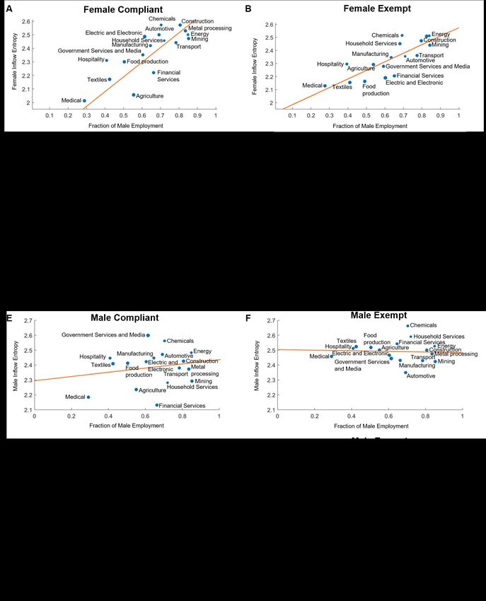
We further investigate whether the Act’s impact differs between industries. We evaluate the relationship
between the percentage of male employment within an industry and the industry’s female labour inflow
diversity and its gender wage gap. We find that male-dominant industries have a higher female labour
inflow diversity and a smaller gender wage gap. This relationship is found to be significantly stronger
among the group of firms who comply with the Act, compared to the group of firms exempt from
the Act. Once again, no significant relationship is found for the male labour inflow diversity. These
results suggest that male-dominant industries are more heavily impacted by the Act as they show greater
adoption of the recruitment strategies used to restructure their workforce and increase female presence
within their workforce.
In the next section we review the related literature on the EE Act, labour mobility, and labour networks.
This is followed, in Section 3, with a discussion of the data used in this study. Next, the methodology
adopted is presented in Section 4. This includes the construction of various networks, the quantification
of inflow diversity, and the layout of our RD design and regression models. In Section 5 our results
are presented, and finally, in Section 6, the conclusion of our study is discussed, along with potential
avenues for future work.
2 Literature review
In this section, the related literature regarding the EE Act, labour mobility, and labour networks is
reviewed.
2.1 The Employment Equity Act
The apartheid regime caused a high level of inequality within the South African labour market by sys-
tematically and purposefully restricting the majority of South Africans from economic and social op-
portunities. Access to skills, formal jobs, and self-employment was racially restricted. An inferior
education system further divided the skills and positions obtained by various groups within the labour
market (Burger and Jafta 2010). This has had a large effect on income distribution and the gender
and racial representation within sectors, occupations, and workforce levels in the South African labour
market (Chimhandamba 2010; Department of Public Service and Administration 1996).
Although much has been done to rectify these effects, the current, non-discriminatory South African
labour market is still socially inequitable, as both black people and women are under-represented in
the better-paying occupations and sectors, and over-represented in low-paid occupations and sectors.
The 1996 Green Paper on Employment Equity (Department of Public Service and Administration 1996)
showed high levels of labour market discrimination. It was found that race and gender (even after con-
trolling for various factors such as education, age, occupation, and sector) were strong factors in deter-
mining an individual’s probability of obtaining work, and predicting their corresponding remuneration.
Whites earn 104 per cent more than blacks, and men receive 43 per cent higher wages than women who
are similarly qualified and working in the same sectors and occupations (Department of Public Service
and Administration 1996).
2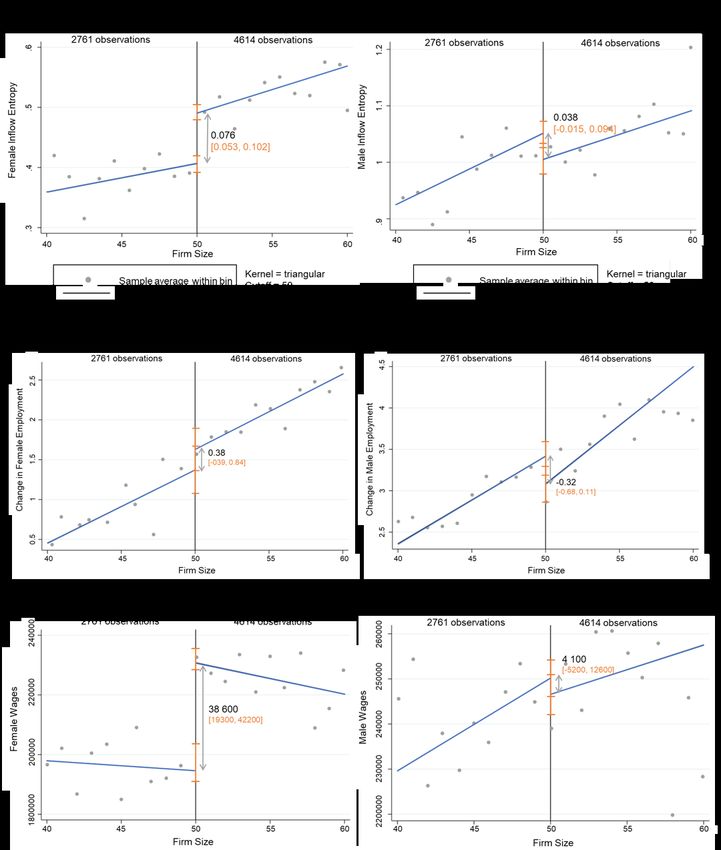
The EE Act, therefore, introduced firm-level affirmative action to enhance the re-entry of blacks and
women into the mainstream of the economy, and accelerate their upward movement into higher-paying
and higher-skilled occupations and sectors. The Act ensures that each firm constructs and abides by a
comprehensive plan, focused on restructuring their workforce to allow for an appropriate representation
of blacks and women within the labour force (conforming to the demographic representation of the
country). Furthermore, a firm’s plan should identify and remove any discrimination in employment
policies and practices (Bowmaker-Falconer et al. 1997; Chimhandamba 2010).

The Act is compulsory for all designated employers. A designated employer is any South African firm
with a workforce greater than 50 employees. However, if a firm has a workforce with fewer than 50
employees but generates an annual revenue above a certain threshold (dependent on the industry in
which the firm operates), the firm is also classified as a designated employer (Department of Public
Service and Administration 1996). The following industries are exempt from the Act: the South African
Defence Force, the Secret Service, and the National Intelligence Service.

Advocates of the Act say that preferential policies break down negative views about previously disadvan-
taged individuals by allowing them to demonstrate their capabilities (Collins 1993). Many economists
also argue that market forces alone are unable to solve the problem of discrimination and therefore an
act changing structural labour market characteristics is vital (Visagie 1999). Critics, however, argue
that the EE Act has led to brain drain (Horwitz 2013) as it incentivizes the emigration of the skilled
minority population. The Act has also been blamed for reducing the productivity of firms by lowering
the general standards of labour and thereby increasing the cost of doing business (Burger 2014; Kruger
and Kleynhans 2014). It is also criticized for reducing foreign investment in South Africa (Dongwana
2016). Furthermore, it has led to many high-skilled vacant jobs or under-skilled employees, as there is
limited labour supply meeting both the requirements of the Act and the requirements of the job (Horwitz
2013).

There is limited academic work analysing the impact of the EE Act on the labour market (Horwitz and
Jain 2011). Most previous research is qualitative and case-study based (focusing on an industry, firm, or
region (Public Service Commission 2006)). Existing studies that do have a quantitative component tend
to focus on high-level aggregate statistics and do not consider lower-level structural properties of the
labour market. For example, an increased representation of previously disadvantaged individuals has
been observed within managerial positions and both higher-paid and higher-skilled occupations since
the implementation of the Act (Public Service Commission 2006). To the authors’ knowledge, there is
no academic research that has investigated the impact of the Act on labour market flow patterns. Labour
flows are a useful tool to evaluate the health of an economy, particularly regarding labour market par-
ticipation and productivity. The EE Act is focused on increasing the participation of under-represented
groups in the labour market, which implies specific changes in labour flow dynamics. Quantifying these
changes is therefore a fundamental part of evaluating the Act’s efficacy.

2.2    Labour mobility

In this section, we review the literature on labour mobility, focusing on the South African context and
differences between genders.

Labour mobility in South Africa

Labour mobility has been an ongoing topic of interest among both social and economic researchers since
the emergence of market societies (McNulty 1980). The study and regulation of labour markets is para-
doxical as it involves the concern of both a well-functioning labour market and people’s welfare.

                                                   3
Although labour mobility is a defining characteristic of an economy, it needs to be well understood
within its context. High labour mobility is often attributed to a strong economy, because an immobile
labour market leads to high rates of structural unemployment (Schioppa 1991). High mobility also
enhances innovation and expansion by making it easier for firms to expand into new markets and attract
qualified labour (Esping-Andersen and Regini 2000). It also creates resilience within the labour market
by allowing workers to be more flexible and adaptable to economic shocks (Diodato and Weterings
2015). On the other hand, high labour mobility may be problematic for an economy. It may prevent
the formation of specialized knowledge (Diodato and Weterings 2015), and lead to job insecurity and
workers who struggle to cope with the impact of change (Pizzati and Funck 2002). Without policy
intervention, high mobility is shown to enhance the downward vertical movement of the lower-educated
workforce, which increases inequality within society.

Policy interventions are aimed at controlling the degree of labour mobility within an economy. These
include the national level of education and skills, the national minimum wage, regulations around the
hiring and firing of workers, bargaining powers and contracts negotiated by trade unions, the presence
of zero-hour contracts, and unemployment protection grants, among many others (Esping-Andersen and
Regini 2000; Pizzati and Funck 2002). The labour market is traditionally studied through a neoclassical
framework. This consists of quantifying labour demand and supply in order to evaluate a labour market
equilibrium. Labour demand is studied through worker flows and labour supply through job flows (gross
creation and destruction of jobs). The impact of labour market regulations is then evaluated through
determining its impact on the labour market equilibrium. The dominant view in the literature is that
increased labour market regulations lowers worker flows (Bassanini et al. 2010; Pries and Rogerson
2005).

In South Africa, labour mobility has primarily been studied through survey data. Most of these studies
have focused on changes in participation and employment rates (Casale et al. 2004), focusing on tran-
sitions in and out of formal employment (Banerjee et al. 2008; Cichello et al. 2005). The first study to
quantify the labour demand and supply within the South African labour market was done by Kerr et al.
(2014), who used the Quarterly Employment Survey (QES) firm data to quantify the level of job creation
and destruction in firms in South Africa. It was found that firms typically create or destroy around 20
per cent of their total jobs annually. Kerr (2018) then continued his analysis using a new administrative
tax dataset (the same dataset used within the current study) to quantify the flow of jobs, workers, and
churning in South Africa. It was found that worker flows, between formal firms, were around 53 per cent
for the 2011–14 period. This is substantially higher than what was previously thought due to the high
levels of unemployment and the high labour regulations within the South African labour market (Baner-
jee et al. 2008; Go et al. 2009). Worker flows were also found to be highly heterogeneous across various
factors. These include firm size, firm earning rates, worker earning rates, and firm industries.

Within our study, we are interested in how the EE Act has influenced inter-industry worker flows. Kerr
investigated worker flows within 34 industry sectors (flows between firms in the same industry sector).3
The largest worker flows were found within the following three industries: 93 per cent in ‘manufactur-
ing’, 79 per cent in ‘household services’, and 72 per cent in ‘hospitality’. On the other hand, the smallest
worker flows were found within the following three industries: 20 per cent in ‘public administration’,
35 per cent in ‘mining and quarrying’, and 37 per cent in ‘electricity, gas, and water’ (Kerr 2018).

3The industry sectors were classified according to a high-level SARS (South African Revenue Service) industry classification
measure.

                                                             4
Gendered labour mobility and the gender wage gap in South Africa
Various socio-economic factors affect the mobility and participation rate of women within the labour
market.4 The main factors in the literature include the level of economic development, the level of
female educational attainment, social dimensions (such as social norms influencing marriage, fertility,
and the woman’s role outside the household), access to credit, household and spouse characteristics,
access to childcare and other supportive services, and institutional setting (e.g. laws, protections, and
benefits) (Gaddis and Klasen 2014; Jaumotte 2004). The U-shaped relationship between economic
development and women’s labour force participation is one of the most well-studied relationships in the
literature (Gaddis and Klasen 2014).5
Policy reforms focused on increasing the overall participation and mobility of female workers aim at
influencing one of these above-mentioned factors. Long-term policy reforms often focus on increas-
ing female education and improving female labour market conditions and norms. Some key short-term
policy reforms include: allowing flexible working-time arrangements or part-time work, removing tax-
ation policies that negatively influence work-sharing decisions (e.g. taxation where second earners in
a household are taxed more heavily), enabling parental leave (up to a certain duration) and childcare
subsidies, enhancing the growth of the service sector, and loosening immigration policies as they reduce
the relative cost of childcare (Buchanan et al. 2011).
South Africa’s female participation rate is 48.77 per cent for 2019, which is lower than the male partic-
ipation rate of 62.59 per cent (Burger and Jafta 2010). However, Casale (2004) showed that the South
African labour market has become feminized in the post-apartheid years. The female share of employ-
ment increased from about 38 per cent in 1994 to about 44 per cent in 2018 (Burger and Jafta 2010).
The increase is believed to be particularly influenced by an increased level of education among women
(Spaull and Broekhuizen 2017) and a reduction in gender biases within the labour market (Oosthuizen
2006). Various pieces of anti-discrimination legislation have been implemented by the South African
government, including the Labour Relations Act No. 66 of 1995 (which sets guidelines for the inter-
actions between employers and employees), the Basic Conditions of Employment Act No. 75 of 1997
(which regulates working conditions and sets a minimum wage for employees in different sectors), and
the Employment Equity Act considered within this study (Burger and Jafta 2010; Leibbrandt et al. 2010;
Ntuli 2007; Posel and Rogan 2014).
Despite an increase in female participation, differences in the quality of employment between genders
persist. Women are over-represented in low-paying occupations and sectors and under-represented in
high-paying occupations and sectors. A gender wage gap was found in the South African labour market
(Burger and Jafta 2010; Casale and Posel 2011; Muller 2009; Ntuli 2007). The average wage gap
has decreased from about 40 per cent in 1993 to about 16 per cent in 2014 (Mosomi 2019). However,
Mosomi found that there was heterogeneity within the trend of the wage gap across the wage distribution.
Most of the decline was found among the lowest-paid workers (below the 10th percentile), attributed to
minimum wage policy implementation in low-paying industries. There has been no significant change in
the gender wage gap at the median, which remains around 23–25 per cent. The 90th percentile showed a
decline in the gender gap between 1993 and 2005; however, this trend has reversed in subsequent years
(Mosomi 2019).
4The labour force participation rate is the proportion of the country’s working-age population that actively engages (either by
working or seeking work) in the labour market (Jaumotte 2004).
5 The U-shaped hypothesis between female participation rates and economic development states that female participation rates
are highest in poor countries where women are engaged in subsistence activities; the participation rate then decreases among
middle-income countries where most jobs are within industries that benefit men. However, as education levels improve and
fertility rates fall, women re-enter the labour force in response to growing demand in the service sector (Gaddis and Klasen
2014).
52.3 Labour flow networks and network tools
The labour networks constructed and the network analysis tools used in this study are reviewed in this
section.
Labour flow networks
Using networks as a modelling tool has become popular in biology, social sciences, and economics
over the last decade. Network analysis has given us the tools to study complex systems.6 It enables the
understanding of the underlying interconnected structure of a system. The popularity of network analysis
stems from the growing availability of micro-data and the increases in computational power that have
made network construction and analysis possible in many cases (Guerrero and Axtell 2013). In this
study, we construct three networks: the inter-firm labour flow network, the inter-industry labour flow
network, and the skill-relatedness network (a normalized inter-industry labour flow network).
In labour economics, labour flow networks have primarily been used to understand the structure and
topology of a labour market. Guerrero and Axtell (2013) were the first to construct an inter-firm labour
network. This is a network in which the nodes represent firms and the edges represent the number of
workers who transition between the corresponding firms.
Inter-industry labour networks, however, first emerged from the related diversification literature within
evolutionary economic geography. The network has mainly been used for modelling and predicting
regional diversification paths (Boschma 2017). Within this literature, Neffke and Henning (2013) were
the first to construct an inter-industry labour network. This is a network in which each node represents
an industry and each edge the number of workers who transition between the corresponding industries.
A skill-relatedness network was then constructed in order to quantify the level of skill overlap between
industries. This network is one in which each node also represents an industry; however, each edge now
represents the skill-relatedness between the corresponding industries. The skill-relatedness is the skill
and knowledge overlap between two industries quantified through normalized labour flows. Relying on
labour flows as a measure of skill-relatedness is based on the assumption that workers have the incentive
to move to industries where their skills are valued. Concurrently, firms are more willing to recruit
workers from other industries who have relevant skills. Therefore, the greater the number of workers
who move between two industries, the higher their skill similarity. However, the size of labour flows
depends on the size of employment within the corresponding pair of industries. Therefore the worker
flows are normalized to take employment size into account.
Skill-relatedness networks have been constructed for various countries, including Sweden (Neffke et
al. 2011), Germany (Neffke et al. 2017), Ireland (O’Clery et al. 2019), the Netherlands (Diodato and
Weterings 2015), and the United Kingdom (unpublished data). To the best knowledge of the authors, no
skill-relatedness network has been constructed for an African economy.
Network analysis tools
This analysis uses three main network analysis tools: centrality measures, information entropy, and
community detection. Each is briefly discussed.
Centrality measures are often adopted in order to analyse the connectivity of a network. A centrality
measure quantifies the relative importance of a node within a network by taking the structure of the
network into account. There are many centrality measures within the literature that vary according to the
amount of local or global information they include about the structure of the network. The in-strength is
6 Here, a complex system is a system of many interrelated parts that influence its overall behaviour.
6a local centrality measure. It sums the weight of all edges that point towards a node (only considering the
direct neighbourhood of a node). It then ranks all nodes by their total strength. In our analysis we wish to
measure the diversity of labour inflows. This measure cannot be used, as all industries within the inter-
industry labour network are not skill-equidistant from each other. To elucidate this problem, consider the
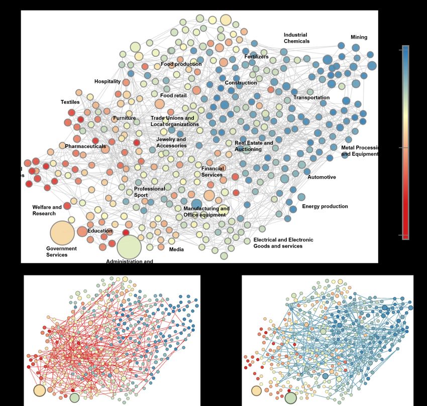
intensive care hospitals industry and the veterinaries industry shown in red in Figure 1(a). Both of these
industries receive workers from two different industries and by using the in-strength centrality measure,
should have similar labour inflow diversities. The intensive care hospital industry, however, receives
workers from two industries that also share a high degree of labour flows. This industry is therefore
less diverse. In-strength centrality is unable to consider a greater degree of network structure and can
therefore not rank the two industries accordingly.
We could also consider a more global network centrality measure that takes a larger amount of the
structure of the network into account (e.g.. the Katz centrality), but as all industries are not defined at
equal levels of granularity this will not provide reliable results. To illustrate this problem, consider the
specialist medical practices industry and the livestock farming industry shown in Figure 1(b) and (c).
Note the difference in the level of detail with which each of these industries’ neighbours are defined.
Although the first industry receives workers from more industries, we cannot argue that it is more diverse
as this could merely be a result of the heterogeneity of the level of detail with which the industries are
defined.
Figure 1: Mock example of various industries and their direct neighbours within the inter-industry labour flow network illustrat-
ing that (a) all industries are not skill-equidistant and (b,c) are defined in varying levels of detail within the original industry
classification
Notes: the industry considered is illustrated in red. The number inside the industry counts the number of different industries
from which it receives workers.
Source: authors’ illustration.
In order to measure the diversity of labour inflows reliably, we therefore adopt an entropy-based measure.
Information entropy is traditionally found in statistical physics. It quantifies the amount of uncertainty
about an event before it occurs, or the amount of information gained about the system once the event
has occurred (Guevara et al. 2003). A low-probability event carries more information than a high-
probability event when it occurs, and therefore a higher entropy. The amount of information that is
obtained from each event becomes a random variable whose expected value is the information entropy.
In the economic literature, Eagle et al. (2010) created an entropy-based measure to quantify the diversity
of an individual’s social interactions with different income levels in the population. The entropy measure
was applied on a network consisting of cellular phone calls between individuals. Our study adopts a very
similar entropy-based metric in which the diversity of labour inflows is measured according to the degree
of different sectors from which an industry or firm hires workers.
In order to detect the various sectors, we construct a new industry classification by clustering the skill-
relatedness network. Community detection techniques have been used extensively to study the structure
and dynamics of biological, social, engineering, and economic networks (Girvan and Newman 2002). A
community or cluster can be defined as a densely connected group of nodes with sparse connections to
other clusters. The problem of community detection consists of partitioning the nodes within a network
into several non-overlapping clusters. Most well-known community detection algorithms seek to find
7a single partition under a particular optimization strategy (Newman 2003). Within this study, we use a
dynamical community detection algorithm, the Markov stability algorithm (Delvenne et al. 2010). The
algorithm is based on diffusion dynamics and uses its properties to unveil the modular structure of the
network. It partitions the skill-relatedness network into ‘dynamical skill-basins’ (O’Clery et al. 2019),
which are groups of industries in which workers freely transition but rarely leave.
3 Data
This study uses an administrative dataset constructed from anonymized tax records for the period 2011–
14 (Ebrahim and Axelson 2019; Pieterse et al. 2018) to count inter-industry and inter-firm worker transi-
tions. The dataset was recently made available to researchers by the National Treasury and SARS.
More specifically, the dataset was constructed from IRP5 tax certificates. These certificates are issued
by an employer who is registered for pay as you earn (PAYE) tax, on behalf of an employee. Each
certificate contains details of the employee, the employer, and the duration and terms of employment.
Note that the dataset only contains workers and firms in the formal economy.7 The reader is directed to
Appendix A1 for a more detailed discussion on the data and the data-cleaning strategy used.
To construct an inter-industry labour flow network, we need to consider how firms are classified into
industries. Within the dataset, a firm is assigned an industry classification code according to their pri-
mary economic activity. The industry codes are a four-digit code that abides by an internally set SARS
classification system. Within the classification system there are 388 different four-digit industry codes.
The codes closely correspond to the ISIC (International Standard Industrial Classification) Revision 4
classification.
In this study, we divide the firms into two groups according to whether a firm is exempt or complies
with the EE Act. Recall that the Act only applies to firms with a workforce of more than 50 employees.
However, firms with annual revenue above a certain threshold are still obliged to comply with the Act
even if their workforce contains fewer than 50 employees. There are also various industries (the South
African Defence Force, the Secret Service, and the National Intelligence Services) that are completely
exempt from the Act. All firms and their workforces that are exempt from the Act are grouped as our
control (exempt) group; all other firms and their workforces are grouped as our treatment (compliant)
group. We have 95,156 firms within our control group and 17,138 firms within our treatment group.
Although there are fewer firms within the treatment group, they contain many more employees.
4 Methodology
In this section we first discuss the construction of three different networks: the inter-firm labour flow
network, the inter-industry labour flow network, and the skill-relatedness network. We then consider
the construction of our inflow entropy measure. This also includes partitioning the skill-relatedness
network and creating a new industry classification. Next, the variables used throughout the study are
defined. Finally, details regarding the RD design and the multivariate regression analysis adopted are
discussed.
7The exclusion of the informal economy does not significantly skew our results as only 30 per cent of all employment in South
Africa is attributed to the informal economy. This is significantly less than in other developing countries (Magruder 2012).
84.1 Network construction
We use the administrative data, discussed in Section 3, to construct the inter-firm labour flow network,
the inter-industry labour flow network, and the skill-relatedness network. The inter-firm labour flow
network is a network in which each node represents a firm and each edge the number of workers who
transition between the two corresponding firms. For the inter-industry labour flow network, each node
represents an industry and each edge the number of worker transitions between the two corresponding
industries. The skill-relatedness network is a network in which each node represents an industry and each
edge is a measure of the skill similarity between the two corresponding industries. The skill similarity
is calculated by comparing the number of worker transitions between two industries compared to what
we expect at random. The differences among these three networks are summarized in Table 1.
Table 1: Properties of the three different networks constructed in this study
Nodes Edges Size of Usage of network
represent represent network in this study
Inter-firm Average number of work transitions Quantify the diversity of labour
Firm 112,294
labour flow network between firms per year flow for firms
Inter-industry Average number of work transitions Quantify the diversity of labour
Industry 388
labour flow network between industries per year flow for industries
Construct a new industry
Skill-relatedness network Industry Skill overlap between industries 388
classification
Source: authors’ illustration.
Let LF (i, j,t) denote the observed labour flows from firm i to firm j between years t and t + 1. We define
the positive and non-symmetric adjacency matrix AF for the inter-firm labour flow network as:
1
AF (i, j) = ∑ LF (i, j,t) (1)
4 t=2011:2014
Furthermore, let LI (i, j,t) denote the observed labour flows from industry i to industry j between years
t and t + 1. We define the positive and non-symmetric adjacency matrix AI for the inter-industry labour
flow network as:
1
AI (i, j) = ∑ LI (i, j,t) (2)
4 t=2011:2014
Both networks are weighted directed graphs.8 In this study, these networks are used to calculate the
labour flow diversity for a firm or industry.
We use various subgraphs of the inter-firm and inter-industry labour flow network within our analysis.
We construct these subgraphs using the same method; however, we only use a subset of LF or LI , where
we only include the transitions of workers who meet certain criteria. The criteria comprise whether the
workers are male or female and whether they transition to firms who either comply or are exempt from
the EE Act. The adjacency matrices of these subgraphs are denoted as Ab,ca , where a ∈ {F, I} indicates
whether we are constructing an inter-firm or inter-industry labour flow network, b ∈ {M, F} indicates
whether we are considering male or female workers, and c ∈ {C, E} indicates whether workers who
transition to either compliant or exempt firms are used.
The third network constructed is the skill-relatedness network. The construction follows the method of
Neffke and Henning (2013). First, the skill overlap between industries is quantified using the labour
flows between them. Within this framework, the existence of large labour flows between a pair of in-
dustries shows that these industries are highly skill-related. However, the size of the two industries
8 A weighted directed graph is a graph in which the edges have both direction and weight.
9influences the size of the labour flows. Therefore, the labour flows are compared to a null model (the ex-
pected labour flows between two industries at random). The null model is a configuration model (Molloy
and Reed 1995). Each edge is the number of labour flows you would expect at random when reconstruct-
ing the graph by shuffling its edges but keeping the total number of labour inflows and outflows of each
industry constant.
The skill-relatedness between industry i and j between years t and t + 1 is given by:
LI (i, j,t) ∑i j LI (i, j,t)
SR(i, j,t) = (3)
∑i LI (i, j,t) ∑ j LI (i, j,t)
The value is effectively the level of labour flow that is observed between industry i and j beyond what
is expected at random. Note that if the flow is larger than what is expected at random, then SR(i, j,t) ∈
[1, ∞). However, if the flow is smaller than what is expected at random, then SR(i, j,t) ∈ [0, 1]. This
measure is highly skewed. Therefore, a transformation is applied to symmetrically map the values onto
the interval SR(i, j,t) ∈ [−1, 1],
SR(i, j,t) − 1
S̃R(i, j,t) = (4)
SR(i, j,t) + 1
where the value of zero represents what is expected at random. Finally, the measure is averaged over the
analysis period 2011–14,
1
M S̃R(i, j) = ∑ S̃R(i, j,t) (5)
4 t=2011:2014
and made symmetric,
M S̃R(i, j) + M S̃R( j, i)
SSR(i, j) = (6)
2
The skill-relatedness network is then constructed by only taking the positive part of SSR(i, j). Therefore,
the edges within the network only include labour flows that are greater than what is expected at random.
We define the positive and symmetric skill-relatedness adjacency matrix ASR as:
(
SSR(i, j), if SSR(i, j) > 0
ASR (i, j) = (7)
0, otherwise
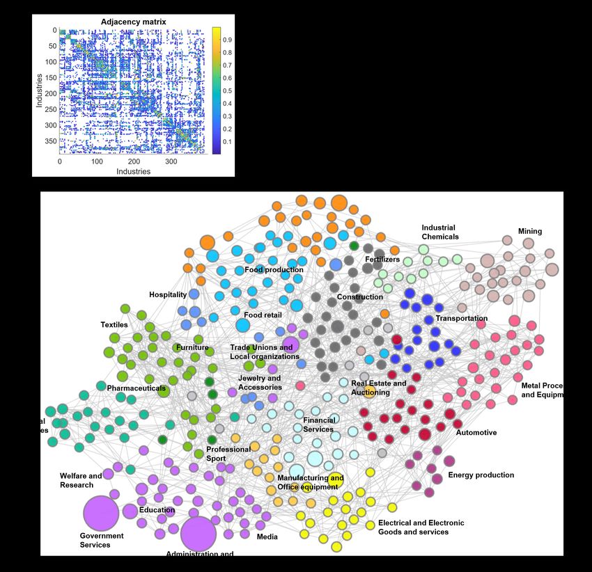
ASR is shown in Figure 2(a). We can see that the matrix is sparse, and there are clear clusters of values
near the diagonals. This shows that there is high skill-relatedness between industries in the same sector
(industries are ordered according to sector). The top 10 industry pairs with the highest skill-relatedness
are shown in Figure 2(b). Note that these industries fall within a wide range of sectors. The skill-
relatedness network is illustrated in Figure 2(c). In this figure, each node represents an industry, the
size of a node represents the average size of the industry, and the weight of each edge represents its
skill-relatedness. The node layout used is a spring algorithm called ‘Force Atlas’ (Jacomy et al. 2014)
in Gephi, which positions industries that are more skill-related closer together. The algorithm simulates
a physical system in which nodes, representing charged particles, repulse each other and edges, repre-
senting springs, attract their nodes. The various forces create a movement that converges to a balanced
state that is then used as the final network configuration. Note that the network displays a high degree
of clustering of related industries. We have added labels indicating the general position of sectors in the
figure.
10Figure 2: (a) The adjacency matrix of the skill-relatedness network. (b) The top 10 industry pairs of the skill-relatedness network
by edge weight. (c) Visualization of the skill-relatedness network for South Africa
Notes: (c): each node represents an industry and each edge the skill-relatedness between the corresponding industry pair.
Nodes are sized by the average employment over the 2011–14 period and coloured according to their industry cluster detected
according to the Markov stability algorithm (t = 0.5). Only edges above a skill-related index of 0.6 are shown. The node layout
is based on a spring algorithm called ‘Force Atlas’ in Gephi.
Source: authors’ compilation based on data.
We use the skill-relatedness network in our study to identify the labour pools within the South African
labour market and construct a new industry classification. We then use this for our inflow entropy
measure. Recall from Section 2.3 that the original industry classification is not used because industries
are not skill-equidistant and defined at different levels of granularity within this classification.
4.2 Constructing a new industry classification
We partition the skill-relatedness network into labour pools. We adopt the methodology of O’Clery et
al. (2019), who use the Markov stability algorithm (Delvenne et al. 2010) as a dynamical clustering
algorithm to unveil labour pools within the Irish labour market. The labour pools represent ‘dynamical
skill-basins in which workers can freely move but rarely leave’ (O’Clery et al. 2019).
11The Markov stability algorithm (Delvenne et al. 2010) is a dynamical community detection algorithm
based on diffusion dynamics. It differs from a static community detection algorithm in that it produces
a range of partitions at different scales (from a few large clusters to many well-defined clusters). This
allows for a more natural understanding on how partitions are constructed. It also unveils the hierarchical
structure of the labour market.9 The range of partitions can also be considered as different aggregation
levels within an industry classification.
The Markov stability algorithm is aimed at maximizing the probability that a random walker remains
in the community in which it started during a time interval. It can be intuitively understood by con-
sidering a random walker wandering on a network (jumping from node to node). The propensity with
which the walker jumps between two nodes is proportional to the corresponding edge’s weight. To dis-
cover a community, the core idea is that if the walker gets trapped in a group of nodes for an extended
period it indicates that there is high connectivity between the group of nodes and thereby a commu-
nity exists. The longer the random walker is observed, the more it can wander and therefore the larger
the node aggregations that result. Hence, changing the time results in different sizes of communities.
For a detailed explanation of the workings of the Markov stability algorithm, the reader is referred to
Appendix A2.
Within our study we choose a single partition as the new aggregation for our industry classification. To
evaluate which of the partitions are most representative of the actual sectors within the economy, we
calculate the robustness of each partition obtained and choose the one with the highest robustness. The
robustness of a partition is a measure of the variation in the resulting partitions obtained when continu-
ally applying the community detection algorithm. We use the variation of information measure (Meila
2003) to quantify the variation. The partition with the lowest variation is chosen as our new industry
classification. A partition containing 21 skill-related industry clusters is suggested by the Markov stabil-
ity algorithm on the South African skill-relatedness network. The partition is illustrated in Figure 2(c)
via the colour of the nodes. We also compare the modularity of our new industry classification and the
original SARS industry classification. Modularity is a measure of how well a partition divides a network
into communities by comparing the number of edges within a community compared to what is expected
at random. Our new industry classification results in a higher modularity, and is therefore an improved
partitioning of the network.
The resulting partition is used as the new industry classification that groups industries into sectors. Note
that this classification considers both the level of skill-relatedness between industries (by quantifying the
skill-relatedness between industries) and corrects for the heterogeneous SARS industry classification (by
allowing industry clusters to be of varying sizes).
4.3 Constructing the inflow entropy measure
Finally, we can measure the diversity of labour flows for either a firm or an industry by measuring the
array of different sectors (previously defined) from which a firm or industry hires workers. We therefore
need to consider both how many different sectors a firm or industry’s workforce flows from, and the
number of workers that flow from each.
In order to quantify the diversity, we construct the inflow entropy measure. The entropy of a random
variable, denoted by H, is a measure of uncertainty and quantifies how much we know about a variable
before observing it. For a discrete random variable X, containing n possible states and a probability
9 Note that the resulting partition from the Markov stability algorithm is only closely but not strictly hierarchical.
12mass function p(x), the entropy is defined as
n
H(X) = − ∑ p(x j ) log(p(x j )) (8)
j=1
The entropy value H(X) lies within the interval 0 ≤ H(X) ≤ log(n). H(X) is minimal when X is deter-
ministic (there is no uncertainty about the variable). The maximal value is obtained when the probability
mass function is a uniform density, p(x) = 1/n.
We now apply entropy to our problem. We let H(XiA ) be the inflow entropy of node i in the network
represented by adjacency matrix A. The discrete random variable X is the skill cluster or sectors from
which node i receives workers. As there are 21 different skill clusters in our new classification, n = 21.
Let sc(i) denote the skill cluster to which node i belongs. We define
e ji
p(XiA = x j ) = N
∑ j=1 e ji (1 − δ (sc( j), sc(i)))
where δ is the Kronecker delta. This represents the fraction of node i’s worker inflows that come from
skill cluster j (excluding the flows in the skill cluster of node i). The inflow entropy is then given
as
21
e ji e ji
H(XiA ) = − ∑ N log( N ) (9)
j=1, j6=sc(i) ∑ j=1 e ji (1 − δ (sc( j), sc(i))) ∑ j=1 e ji (1 − δ (sc( j), sc(i)))
Therefore, the larger the array of different skill clusters a firm (or industry) workforce flows from,
the higher their inflow entropy. We rewrite H(XiA ) = Hi (A), and use this notation in the rest of this
paper. To obtain the male and female, as well as exempt and compliant, inflow entropies we apply this
methodology to our various subgraphs.
4.4 Variable construction
Within this study, we investigate the impact of the EE Act on the diversity of labour flows (inflow
entropy) and the gender wage gap. We investigate these factors on both a firm and industry level.
Recall from Section 4.3 that the inflow entropy is denoted as Hi (Ab,c
a ), where i is the unit under inves-
tigation (either a firm or industry). Furthermore, a ∈ {F, I} indicates whether a firm- or industry-level
analysis is being adopted, respectively. Additionally, b ∈ {M, F} indicates whether only male or female
worker flows are considered, respectively. Finally, c ∈ {C, E} indicates where flows into firms who
comply with the Act or are exempt from the Act are being investigated.
Similarly, let the average wage be denoted as Wab,c (i), where the subscripts and superscripts have the
same meaning as in the inflow entropy measure. The gender wage gap, defined as the percentage differ-
ence between the male wage and the female wage, is then denoted as
W Gca (i) = (WaM,c (i) −WaF,c (i))/WaM,c (i)
Furthermore, the employment size within the time period t is denoted as Ei (Ab,c
a ,t) and the fraction of
male employment FMEi (Aca ,t), where
FMEi (Aca ,t) = Ei (AM,c F,c M,c
a ,t)/(Ei (Aa ,t) + Ei (Aa ,t))
When a superscript is omitted this is indicative that all states (the union of all states within the set) are
considered. Next, we discuss the construction of our RD design to determine the impact of the EE Act
in our study.
134.5 The RD design
An RD design is a well-known policy evaluation method that has emerged as one of the most credible
non-experimental strategies for the analysis of causal effects (Cattaneo et al. 2019). An RD design
exploits a discontinuity in the treatment assignment to identify causal effects (Cattaneo et al. 2019;
Imbens and Lemieux 2008). We use an RD design within our study to determine the impact of the EE
Act on a firm’s male and female labour flow diversity and a firm’s average gender wage gap.
Within our RD design, our independent variable is the size of employment within a firm. Following the
legislation of the EE Act, firms with more than 50 employees comply with the Act, while those with
fewer than 50 employees are exempt from the Act. Note that firms who have fewer than 50 employees but
still abide by the Act as their annual revenue is above the threshold value are removed from our sample
to prevent skewing of our results. The key feature of the design is that the probability of complying with
the Act changes abruptly, from 0 to 1, at the 50-employees cutoff value. The discontinuous change in
the probability is used to learn about the local effect of the Act on the dependent variable (which is the
male and female inflow entropy (Hi (Ab,c F ) where b ∈ {M, F} and c ∈ {C, E}) and the average male and
M,c F,c
female wage (WF (i) and WF (i) where c ∈ {C, E})). Therefore, firms that are just below the cutoff
(have a firm size of 49) are used as a comparison group for firms just above the cutoff (have a firm size of
51). As the sizes of these firms are very similar, it is expected that without the Act the outcome variable
of these two groups should be very similar. A significant discontinuity found between these two groups
is indicative of the impact of the Act.
To estimate the discontinuity, we fit a polynomial function to the data on each side of the cutoff. We
adopt a local linear polynomial approach and choose a polynomial of order 1. We do not choose a
higher-order polynomial, as these polynomials provide poor approximations at boundary points (this
is also known as the Runge phenomenon in approximation theory (Trefethen 2013)). However, the
problem with choosing a lower-order polynomial is that the size of the neighbourhood (the interval) that
is considered within the analysis heavily influences the result. We therefore chose a bandwidth based on
the algorithm of Imbens and Lemieux (2008), which chooses an optimal bandwidth that minimizes the
asymptotic bias and variance of the local linear polynomial estimator. Therefore, in choosing a linear
regression function with a suitable bandwidth, we allow for a fit that is less sensitive to over-fitting and
boundary problems.
Furthermore, we adopt a triangular kernel function that assigns non-negative weights to each observation
based on its distance to the cutoff. The largest weight is assigned to the values at the cutoff. The
weight then symmetrically and linearly decreases as values are further from the cutoff (Cattaneo et al.
2019).
More formally, the independent variable xi is equal to the firm’s employment size. The dependent
variable is denoted as yi , which is equal to either the inflow entropy (Hi (Ab,c
F )) or the average male and
female wage (WFM,c (i) and WFF,c (i)). The cutoff value is chosen at c = 50; the bandwidth h = 10. In our
linear regression model, yi is then also defined as a linear function of xi as:
(
αR + βR xi + εi , if (c − h) ≤ xi < c
yi = (10)
αL + βL xi + εi , if c ≤ xi ≤ (c + h)
The values of the coefficients are then determined by using the triangular kernel function for weighted
least square regression by the following optimization function:
xi − c
min ε = (1 − | |) × (yi − (α + β xi )2 ) (11)
h
Finally, the RD treatment effect is calculated by determining the vertical distance at the cutoff point:
τRD = lim E[yi |xi = c] − lim E[yi |xi = c] (12)
R L
x−
→c x→
−c
14It is important to note that regardless of the ability of the RD design to show causal effects, the RD
design is not a valid measure for representing treatment effects that occur for units much further away
from the cutoff value. It is therefore unable to predict the overall relationship between the two variables
(Cattaneo et al. 2019). Note that the RD design is done at the firm level. Next, we turn to the industry
level.
4.6 Regression analysis
We are interested in investigating how the Act impacts different industries. We hypothesize that male-
dominant industries will be more heavily impacted by the Act and result in a higher female inflow
entropy and smaller gender wage gap.
We therefore investigate the relationship between the fraction of male employment (FME) and the male
and female inflow entropy (H) using a multivariate linear regression model, given by
H(Ab,c c b,c b,c b,c b,c
I ) = α + β1 FME(AI ) + β2 log(E(AI )) + β3 (E(AI , 2014) − E(AI , 2011)) + β4WI ) (13)
where b ∈ {M, F} and c ∈ {C, E}. We control for the impact of the average employment size, the
employment growth across the time period (2011–14), and the average wage of each industry within
the model. The logarithm of the change in employment is not used in order to allow for industries with
negative growth to be included in the model.
Similarly, we investigate the relationship between the fraction of male employment (FME) and the
gender wage gap (W G). The multi-variant linear regression model is given by
W GcI = α + β1 FME(AcI ) + β2 log(E(AcI )) + β3 (E(AcI , 2014) − E(AcI , 2011)) + β3 log(WIc ) (14)
where b ∈ {M, F} and c ∈ {C, E}. We again control for the impact of the average employment size, the
employment growth across the time period (2011–14), and the average wage of each industry.
The regression analysis is performed for both the treatment group (firms that comply with the Act) and
the control group (firms that are exempt from the Act). We then compare the relationships between these
groups.
5 Results
In this section, we investigate the impact of the EE Act on the diversity of male and female labour
flows and the gender wage gap. We first investigate the impact at the firm level using an RD design.
At the industry level, we then investigate whether male-dominant industries have been more heavily
impacted by the Act and therefore display greater diversity of female labour flows and smaller gender
wage gaps.
5.1 Evaluating the impact of the EE Act at the firm level
The resulting RD design, taking the male and female inflow entropy (Hi (AM F
F ) and Hi (AF )) as our out-
come variable (yi ) in Equation (10) is illustrated in Figure 3(a) and (b), respectively. Note that for both
male and female workers, as the size of a firm increases, their inflow entropy also increases. This is
because as a firm increases in size, it typically hires workers from more sectors in order to operate dif-
ferent divisions within the firm. However, as seen in the figure, a large, positive discontinuity is found
for the female inflow entropy at the cutoff value of 50. Using Equation (12), we obtain a treatment effect
of 0.076 with a 95 per cent confidence interval of [0.053, 0.102] for the female inflow entropy. A much
smaller, negative discontinuity is found for the male case. The treatment effect is 0.038 with a 95 per
cent confidence interval of [−0.015, 0.094]. This shows that as a firm (with 50 employees) changes from
15You can also read