Pirates without Borders: The Propagation of Cyberattacks through Firms' Supply Chains - NO. 937 JULY 2020 JULY 2021
←
→
Page content transcription
If your browser does not render page correctly, please read the page content below
Pirates without Borders:
 NO. 937
JULY 2020
            The Propagation of
 REVISED
            Cyberattacks through
JULY 2021
            Firms' Supply Chains
            Matteo Crosignani | Marco Macchiavelli | André F. Silva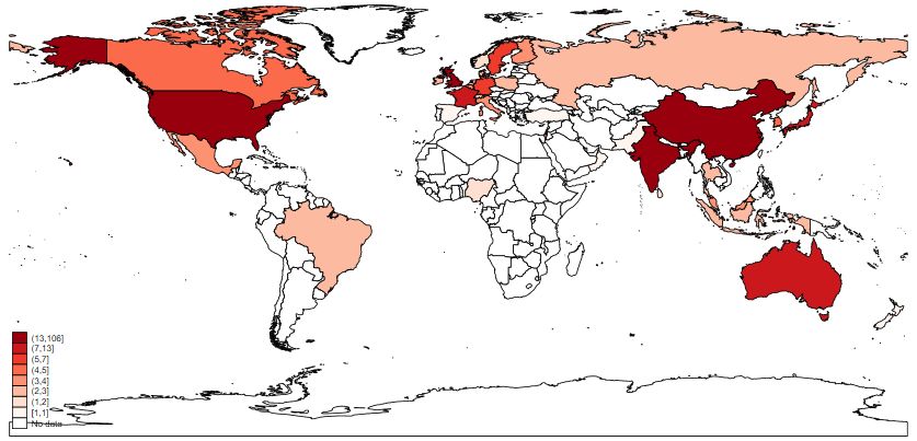
Pirates without Borders: The Propagation of Cyberattacks through Firms' Supply Chains
Matteo Crosignani, Marco Macchiavelli, and André F. Silva
Federal Reserve Bank of New York Staff Reports, no. 937
July 2020; revised July 2021
JEL classification: L14, E23, G21, G32

                                                 Abstract

We document the supply chain effects of the most damaging cyberattack in history. The disruptions
propagated from the directly hit firms to their customers, causing a four-fold amplification of the initial
drop in profits. These losses were larger for affected customers with fewer alternative suppliers. Internal
liquidity buffers and increased borrowing, mainly through bank credit lines, helped firms navigate the
shock. The cyberattack also led to persisting adjustments to the supply chain network, with affected
customers more likely to create new relationships with alternative suppliers and terminate those with the
directly hit firms.

Key words: cyberattacks, supply chains, bank credit

________________

Crosignani: Federal Reserve Bank of New York (email: matteo.crosignani@ny.frb.org). Macchiavelli,
Silva: Board of Governors of the Federal Reserve System (email: marco.macchiavelli@frb.gov,
andre.f.silva@frb.gov). The authors thank Viral Acharya, Tania Babina, Miguel Faria-e-Castro,
Mariassunta Giannetti, Michael Gofman, Huiyu Li, Nicola Limodio, Vojislav Maksimovic, Andreas
Milidonis, Camelia Minoiu, Patricia Mosser, Andreas Papaetis, Brian Peretti, Andrea Presbitero, Julien
Sauvagnat, Stacey Schreft, Antoinette Schoar, Jialan Wang, and conference and seminar participants at
the 2021 NBER Corporate Finance Spring Meeting, London School of Economics, 2020 Federal Reserve
System Conference on Financial Institutions, Regulation, and Markets, 2020 OFR/Cleveland Fed
Financial Stability Conference, EBRD, Federal Reserve Board, NY Fed, University of Sussex, 2020 Bank
of Italy/FRB Conference on Nontraditional Data & Statistical Learning, 2020 EBA Policy Research
Workshop, 2021 SGF Conference, Bank of Italy, ifo Institute - University of Munich, Humboldt
University of Berlin, and 2021 IBEFA Summer Meeting for their comments. They also thank William
Arnesen and Frank Ye for excellent research assistance.

This paper presents preliminary findings and is being distributed to economists and other interested
readers solely to stimulate discussion and elicit comments. The views expressed in this paper are those of
the author(s) and do not necessarily reflect the position of the Federal Reserve Bank of New York or the
Federal Reserve System. Any errors or omissions are the responsibility of the author(s).

To view the authors’ disclosure statements, visit
https://www.newyorkfed.org/research/staff_reports/sr937.html.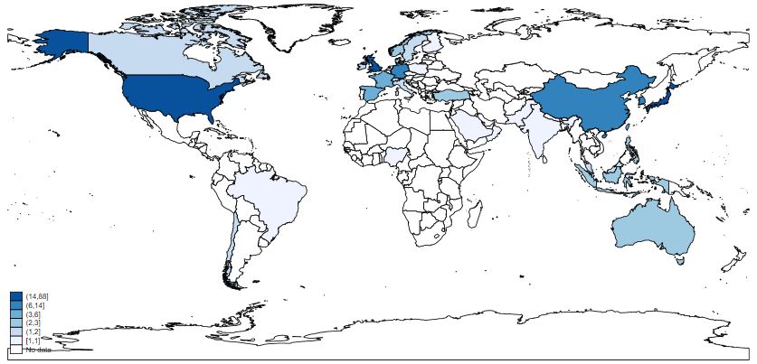
1       Introduction
Cybercrime is now one of the most pressing concerns for firms.1 Hackers perpetrate frequent
ransomware attacks mostly for financial gains, while state-actors often use more sophisticated
techniques to obtain strategic information such as intellectual property and, in more extreme
cases, to disrupt the operations of critical organizations. Cyberattacks that are severe enough
to disrupt the integrity of IT systems can spread instantaneously without warning signs, are
often not geographically clustered, and can ultimately damage firms’ productive capacity
and thus also potentially affect their customers and suppliers. However, despite these unique
features and their growing importance, there is little empirical evidence on the potentially
disruptive effects of cyberattacks on the productive sector.
    In this paper, we study a particularly severe cyberattack that inadvertently spread beyond
its original target and disrupted the operations of several firms around the world. Through
supply chain relations, the effects of the cyberattack propagated downstream to the customers
of directly hit firms.2 To cope with the shock, affected customers used their liquidity buffers
and increased their reliance on external finance, drawing down their credit lines at banks.
We also observe persisting adjustments to the supply chain network in response to the shock,
with affected customers more likely to create new relationships with alternative suppliers and
terminate those with the directly hit firms.
    More specifically, we examine the impact of the most damaging cyberattack in history so
far (Greenberg, 2018, 2019).3 Named NotPetya, it was released on June 27, 2017 and targeted
Ukrainian organizations in an effort by the Russian military intelligence to cripple Ukrainian

    1
     For instance, the latest World Economic Forum Executive Opinion Survey ranks cyberattacks as the
number one risk for CEOs in North America and Europe (WEF, 2019).
   2
     We refer to customers (suppliers) of directly hit firms as affected customers (suppliers) throughout.
   3
     See also a newspaper article (https://www.wired.com/story/white-house-russia-notpetya-attribution/)
and an assessment by Kaspersky (https://www.kaspersky.com/blog/five-most-notorious-cyberattacks/24506/).

                                                    1
critical infrastructure. The initial vector of infection was a software that the Ukrainian
government required all vendors in the country to use for tax reporting purposes. When this
software was hacked and the malware released, it spread across different companies, including
large multinational firms through their Ukrainian subsidiaries. For instance, the shipping
company Maersk had its entire operations coming to a halt, creating chaos at ports around
the globe. A FedEx subsidiary was also affected, becoming unable to take and process orders.
Manufacturing, research, and sales were halted at the pharmaceutical giant Merck, making it
unable to supply vaccines to the Center for Disease Control and Prevention (CDC). Several
other large companies (e.g., Mondelez, Reckitt Benckiser, Nuance, Beiersdorf) had their
servers down and could not carry out essential activities.
  First, we show that the halting of operations among the directly hit firms had a significant
negative effect on the productive capacities of their customers around the world, which
reported significantly lower profits. A conservative estimate implies a $7.3 billion loss by
the affected customers, an amount four times larger than the losses reported by the firms
directly hit by the cyberattack. Faced with this temporary shock, affected customers depleted
some of their pre-existing liquidity buffers and increased the amount of external borrowing,
allowing them to maintain investment and employment. While the downstream disruptions
to customers were severe, we do not find significant upstream effects to the suppliers of the
directly hit firms, nor downstream effects to the customers of the affected customers.
  Second, we investigate the role of supply chain vulnerabilities in driving these effects.
We find that the downstream disruption caused by the cyberattack is concentrated among
customers that have fewer alternatives for the directly hit supplier. This result holds both
when considering how many other suppliers a customer has in the same industry of the directly
hit supplier, and when focusing on suppliers of less substitutable goods and services—that is,
suppliers providing high-specificity inputs.
  Third, we analyze in detail the role of banks in mitigating the negative liquidity effects of
the cyberattack on affected customers. To this end, we use confidential credit register data

                                               2
for the US (i.e., the Y-14Q corporate schedule), with loan-level information at a quarterly
frequency for banks with total assets of more than $50 billion. While there was no change in
credit line commitments granted by banks, affected customers drew down relatively more
on their credit lines to compensate for the liquidity shortages. Interest rate spreads also
increased relatively more for affected customers, a result explained by an increase in risk, as
measured by the expected probability of default that each bank assigns to a given firm.
Finally, we examine the dynamic supply chain response to the disruption caused by the
cyberattack. We find that affected customers are more likely to form new trading relationships
with firms in the same industry as the directly hit supplier after the shock. This result
suggests that the disruption caused by the cyberattack served as a “wake-up call” for the
affected customers which responded by finding alternative suppliers. We also find that
the affected customers are more likely to end their trading relationship with the suppliers
directly hit by the cyberattack, thus suggesting that the temporary disruptions caused by
the cyberattack had long-lasting effects by eroding the reputation of the directly hit firms as
reliable suppliers.
Our paper contributes to the nascent literature on the economics of cybercrime—an area
that is getting increasing attention by both practitioners (Accenture, 2019; Verizon, 2019;
Siemens, 2019; NERC, 2020) and policymakers (US Congress, 2021; Powell, 2021). The
academic literature has mostly focused on examining the effects of cyber risk on financial
stability (Kashyap and Wetherilt, 2019; Duffie and Younger, 2019; Kopp, Kaffenberger and
Wilson, 2017; Aldasoro et al., 2020; Eisenbach, Kovner and Lee, 2021) and developing firm-
level measures of exposure to cyber risk using textual analysis (Jamilov, Rey and Tahoun,
2021; Florakis et al., 2020). Other related papers study abnormal equity returns following
data breaches (Kamiya et al., 2021; Garg, 2020; Akey, Lewellen and Liskovich, 2021; Amir,
Levi and Livne, 2018). While data breaches can lead to reputation, litigation, and other
monetary costs, like most cyberattacks, they usually do not disrupt firms’ operations. In
contrast to these studies, we focus on a far more damaging and larger-scale cyberattack
3resulting in operational disruptions and document its economic and financial effect, through
supply chain linkages, on the productive sector at large. These disruptive cyberattacks are
becoming more and more frequent, as evidenced by the ransomware attacks on Colonial
Pipeline, the largest pipeline system for refined oil products in the United States, and JBS, a
global beef processing company. In these cases, operations halted for several days, causing
protracted supply chain bottlenecks.4
Our paper also complements the literature on the propagation of shocks through supply
chains following severe shocks such as natural disasters (Barrot and Sauvagnat, 2016; Boehm,
Flaaen and Pandalai-Nayar, 2019; Carvalho et al., 2021), pandemics (Bonadio et al., 2021),
and financial crises (Alfaro, Garcı́a-Santana and Moral-Benito, 2021; Cortes, Silva and
Van Doornik, 2019; Costello, 2020).5 Specifically, we show that large supply chain shocks
can lead to a reconfiguration of the supply chain network as customers of directly hit firms
form new trading relationships with alternative suppliers and terminate relationships with
the directly hit firms. These results are especially relevant for the theoretical literature on
endogenous production networks (Elliott, Golub and Leduc, 2020; Taschereau-Dumouchel,
2020; Acemoglu and Tabhaz-Salehi, 2020). Relatedly, the cyberattack we study has several
4
Our paper is also related to the literature on intelligence and espionage. Berger et al. (2013) and Dube,
Kaplan and Naidu (2011) study the effects of CIA influence on trade and stock returns for firms with a
particular interest in regime change, respectively. Martinez-Bravo and Stegmann (2021) use the CIA vaccine
campaign to verify a target’s DNA to show the effects of vaccine distrust on immunization, Ahn and Ludema
(2020) document the effects of sanctions related to the Russian annexation of Crimea, Lichter, Löffler and
Siegloch (2021) examine the effect of state surveillance on civic capital and economic performance, while Glitz
and Meyersson (2020) estimate the economic returns resulting from state-sponsored industrial espionage.
5
Boehm, Flaaen and Pandalai-Nayar (2019) exploit an earthquake in Japan and estimate a near zero
elasticity of substitution of intermediate goods in the short-run, while Carvalho et al. (2021) use the same
shock to map its propagation patterns through supply chains. Barrot and Sauvagnat (2016) document that
suppliers hit by natural disasters propagate the shock downstream as well as horizontally. Costello (2020)
finds that firms facing financing constraints transmit shocks downstream via declines in trade credit. Cortes,
Silva and Van Doornik (2019) show that firms borrowing from more stable funding sources benefit both their
suppliers and customers. Finally, Alfaro, Garcı́a-Santana and Moral-Benito (2021) show how bank credit
supply shocks that affect borrowing firms are propagated downstream to their customers. However, they find
mixed evidence on upstream propagation.
4advantages relative to the more commonly analyzed shocks. On the one hand, natural disasters
tend to follow seasonal and geographical patterns, making the identification particularly
challenging. On the other hand, pandemics and credit supply shocks are often slower-moving
and hit several firms at the same time, causing the effects to be likely driven by both demand
and supply forces. Instead, NotPetya is more unpredictable and faster to materialize, occurs
amid normal economic conditions, and affects different geographical regions.
2 Background on NotPetya
In the intelligence world, few things are what they seem. Petya is the name of a ransomware
that circulated in 2016. The victim was infected after opening a PDF file purporting to
be the resume of a job applicant and, from there, the ransomware encrypted the master
file table which serves as a roadmap for the hard drive, making the data on the computer
unreachable. The victim was then asked to make a Bitcoin payment to get the hard drive
decrypted. What seemed to be a new version of Petya spread quickly in June 2017. It hit
Ukraine the hardest but it also appeared worldwide. However, this new version was able to
spread across networks, without requiring to obtain administrative access. Even though it
appeared to be just another ransomware, as shown in Figure A.1 in the Online Appendix,
it was quickly found out that the real intent was not the financial gain from the ransom
payment. Indeed, the attack was not even designed to keep track of the decryption codes.
Instead, the true intent was to encrypt and paralyze the computer networks of Ukrainian
banks, firms, and government. This was not a new version of Petya.
This cyberattack was the hand of a hacking group from the Russian military intelligence,
the GRU. The Russian government had been actively involved in meddling in Ukrainian
matters since Ukraine, previously part of the Soviet Union, took steps to build closer ties
to NATO. Initially, Russia directed a series of cyberattacks to Ukraine, including its power
grid, and then resorted to military action by invading and annexing Crimea. It should also
5be noted that the timing of the NotPetya attack was in a way serendipitous. The ease with
which NotPetya spread from network to network without human intervention depended on
a never-seen-before piece of code that was leaked in April 2017 by the Shadow Brokers, a
hacking group. The leaked code, called Eternalblue, is a very sophisticated tool developed by
the NSA to harvest passwords and move from network to network. Eternalblue was used
together with another tool, Mimikatz, that was already circulating among hackers and can
find network administrator credentials stored in the infected machine’s memory.6
NotPetya was itself a supply chain attack, in the sense that the initial point of entry was
a backdoor planted in an accounting software, called M.E. Doc, widely used by Ukrainian
firms for tax reporting. As a result, most companies operating in Ukraine got infected,
including multinational companies through their Ukrainian subsidiaries.7 More generally,
Moody’s (2020) argues that companies with less sophisticated cybersecurity are at risk of
attacks stemming from suppliers and vendors with access to their IT systems. For instance, a
compromised software company can become a vector through which thousands of customers’
computers are infected, as in the case of NotPetya.
3 Data
We use several data sources to conduct our analysis at both the firm- and loan-level, including
global supply chain relationships data from FactSet Revere, balance sheet data on firms
worldwide from Orbis, and credit register data for the US from the Federal Reserve’s Y-14Q.
First, to identify the firms directly affected by NotPetya, we start by web scraping
6
Microsoft released a patch for Eternalblue prior to the NotPetya incident. However, NotPetya could
infect unpatched computers, grab the passwords via Mimikatz, and spread to patched computers. Many firms
reportedly do not update regularly for fear that the updates could interfere with their software.
7
More details about NotPetya can be found in Greenberg (2019), a book about NotPetya and other
cyberattacks conducted by Russian military intelligence on Ukraine in 2014–2017.
6Firm Name Costs Additional Details
Beiersdorf $43 mln Various locations of the Beiersdorf pharmaceutical group were cut
Assets: $7.69 bln off from mail traffic for days. Beiersdorf said 35 million euros worth
of second quarter sales were delayed to the third quarter and it was
totting up the costs of the attack for items such as calling in outside
experts, promotions, and using other production sites to make up for
shortfalls.
FedEx $400 mln Delivery service FedEx lost $400 million after NotPetya crippled its
Assets: $33.07 bln European TNT Express business. The reported costs came from loss
of revenue at TNT Express and costs to restore technology systems.
Six weeks after the attack, customers were still experiencing service
and invoicing delays, and TNT was still using manual processes in
operations and customer service.
Maersk $300 mln Maersk reinstalled 4,000 servers, 45,000 PCs, and 2,500 applications
Assets: $68.84 bln over ten days. The company only experienced a 20% drop in volume,
while the remaining 80% of operations were handled manually. Losses
were about $300 million, including loss of revenue, IT restoration costs,
and extraordinary costs. The company was hiring 26 new employees a
week, planning to have 4,500-5,000 IT employees within 18 months. At
Maersk terminals in the Port of New York and New Jersey, computers,
phones, and gate system shut down, forcing workers to use paper
documents.
Merck $670 mln At Merck, NotPetya temporarily disrupted manufacturing, research
Assets: $98.17 bln and sales operations, leaving the company unable to fulfill orders for
certain products, including vaccines. The attack cost Merck about
$670 million in 2017, including sales losses and manufacturing and
remediation-related expenses.
Mondelez $180 mln The global logistics chain of the food company Mondelez was disrupted
Assets: $66.82 bln by NotPetya. The forensic analysis and restoration of all IT networks
cost $84 million. Added to this was the loss of sales. Altogether
Mondelez had to record $180 million of damage by the attack.
Nuance $92 mln NotPetya affected Nuance’s cloud-based dictation and transcription
Assets: $5.82 bln services for hospitals. Nuance estimated a negative impact of $68
million in lost revenues and $24 million in restoration costs.
Reckitt Benckiser $117 mln Reckitt Benckiser was hit by NotPetya, halting production, shipping
Assets: $24.19 bln and invoicing at a number of sites. The British consumer goods
company suffered $117 million in losses, 1% of annual sales.
WPP $15 mln UK multinational advertising firm WPP was hit by NotPetya, costing
Assets: $41.55 bln about $15 million before insurance. The damage was limited by the
fact that WPP’s systems are not fully integrated.
Table 1: Firms Directly Affected by NotPetya. Firms directly affected by NotPetya, total assets,
total reported costs associated with NotPetya, and additional details. Sources: SEC Filings and Dow Jones
Factiva.
7SEC filings in 2017 and 2018.8 We experiment with different keywords, including “Petya”,
“NotPetya”, and “Cyber.” Among the filings that contain a match, we exclude matches that
are unrelated, such as cybersecurity firms citing NotPetya as the main cyberattack of the
year. We also look for instances in which NotPetya is cited in newspaper articles worldwide.
Using the Dow Jones Factiva database that contains a repository of international newspaper
articles, we obtain over 4,500 relevant articles which we manually check for stories of firms
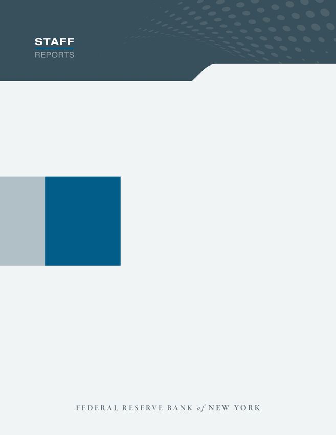
directly hit by NotPetya. Finally, we cross-check the list of directly hit firms with Greenberg
(2019). We exclude firms in Ukraine, Russia, as well as non-public firms that we would not be
able to find in other data sets, e.g., government agencies and hospitals. Overall, as described
in detail in Table 1, we identify 8 public firms that were directly hit by NotPetya—including
FedEx, Maersk, Merck, Mondelez, as well as other very large companies in the US, UK,
Germany, and Denmark.9 In Figure 1, we show that the stock price of these directly hit firms
collapsed by 5% after they disclosed the damages of NotPetya.
Second, we obtain global supply chain relationships data from FactSet Revere, arguably the
most comprehensive source of firm-level customer-supplier relationships currently available.10
Specifically, the data set includes almost a million relationships between large (mostly publicly-
listed) firms around the world. Each customer-supplier relationship has information on the
start date, end date, and relationship type. FactSet collects this information through the
8
Starting in 2005, the Securities and Exchange Commission (SEC) required publicly traded firms to
disclose material factors that may adversely affect their business, operations, or future performance in 10-K
filings (providing updates in the subsequent 10-Qs).
9
We show the geographical distribution of these directly hit firms in Figure A.2 in the Online Appendix.
We do not consider the customers and suppliers of DLA Piper and Saint-Gobain in our specifications since
this information is not available in Factset Revere—in the latter case, supply chain data is only available
after the shock. Other companies reportedly hit by the cyberattack, though to a much small extent, include
the Italian Buzzi Unicem and the German Deutsche Bahn and Deutsche Post. These firms are also excluded
from our analysis due to the lack of supply chain information both before and after the shock.
10
Alternative sources of supply-chain data either do not have information with sufficiently high-frequency
on the start and end dates of a relationship between two firms (e.g., Bloomberg, Capital IQ) or are not as
granular as FactSet (e.g., Compustat Segment data which only reports, with an annual frequency, the largest
customers of a supplier).
8Stock Price of Directly Hit Firms
102
100
Stock Price Index
98
96
94
−6 −4 −2 0 +2 +4 +6
Figure 1: Stock Price of Directly Hit Firms Around News of the Damages of NotPetya. This
figure shows the stock price evolution around the news of the damages of NotPetya (from seven trading days
prior to the news to seven days after the news). Stock prices are averaged across firms and normalized to 100
seven trading days before the disclosure of the news. The dashed lines indicate the standard errors around
the mean. The dates when the news of the damages were publicly released are as follows: August 16, 2017
for Moller-Maersk (link); August 2, 2017 for Beiersdorf (link); June 28, 2017 for Mondelez (link); August
22, 2017 for WPP (link); June 28, 2017 for Nuance (link); July 16, 2017 for FedEx (link); July 5, 2017 for
Reckitt Benckiser (link); October 26, 2017 for Merck (link). Source: Datastream.
firms’ public filings, investor presentations, websites, corporate actions, press releases, and
news reports. Following Gofman, Segal and Wu (2020), we drop redundant relationships
whose start and end dates fall within the period of a longer relationship between the same
firm pair and combine multiple relationships between two firms into a continuous relationship
if the time gap between two relationships is shorter than six months. Using each firm’s
International Securities Identification Number (ISIN), we are able to identify a total of 233
customers and 320 suppliers indirectly affected by the cyberattack, i.e. exposed through their
supply chain connections to directly hit firms.11
Third, we collect balance sheet and income statements information on firms worldwide
11
We show the geographical distribution of affected customers and affected suppliers in Figure A.3 and
Figure A.4 in the Online Appendix.
9from Orbis—a database by Bureau Van Dijk (part of Moody’s Analytics) that contains data
for more than 350 million companies globally. In addition to its extensive coverage, Orbis is
particularly attractive due to its cross-country comparability since the data provider organizes
the information in a standard global format (Kalemli-Ozcan et al., 2019). We merge Orbis
with FactSet using the ISIN of each firm and disregard companies that are not present in
both data sets to avoid selection bias due to the inclusion of smaller listed firms that appear
in Orbis but that do not report supply chain relations. In addition, as it is standard in
the literature, we remove financial firms and firms in the government sector. We obtain an
intersection of 70,590 firm-year observations, corresponding to 15,781 firms from 2014 to
2018, the most recent date available in Orbis.
Finally, we obtain loan-level information on bank credit to firms from the corporate loan
schedule (H.1) of the Federal Reserve’s Y-14Q. These data have been collected since 2012 to
support the Dodd-Frank Act’s stress tests and assess bank capital adequacy for large banks
in the US. The credit register provides confidential information at the quarterly frequency on
all credit exposures exceeding $1 million for banks with more than $50 billion in assets. These
loans account for around 75% of all commercial and industrial (C&I) lending volume during
the period we analyze. In addition to the amount of committed credit for each firm-bank
pair, the data set also contains information on the committed and drawn amounts on credit
lines, the amount that is past due, as well as information on other loan characteristics, such
as the interest rate spread, maturity, and collateral. Finally, we also have information on
each bank’s internal assessment of the default probability of a given firm—a model-based
metric that captures the bank’s hard information about a given borrower and that predicts
loan delinquency (Adelino, Ivanov and Smolyansky, 2020).
In order to identify firms indirectly affected by the cyberattack, we merge these firm-
bank data for the US with Orbis and FactSet using the firms’ tax identification numbers
and CUSIPs available in the Y-14Q. This results in a sample of 137,630 bank-firm-quarter
observations from 2014:Q1 to 2018:Q4, covering 37 banks and 1,997 firms. Of these, 85 are
10customers of firms directly hit by the cyberattack, corresponding to 87% of US customers in
the Orbis-FactSet firm-level sample.
4 Identification Strategy
4.1 Firm-level Analysis
Our goal is to document the effects of the NotPetya cyberattack through the supply chain.
Given that the attack caused the directly hit firms to halt operations for several weeks, we
are interested in estimating the effects on these firms’ customers and suppliers, which we refer
to as affected customers and affected suppliers. We use a difference-in-differences approach,
comparing the change in behavior of firms indirectly affected by the shock through their
supply chain with that of unaffected firms operating in the same industry, country, and size
quartile in the same year. Specifically, we estimate the following specification:
Yijt = α + βPostt × Affectedi + ξi + ηjt + ijt (1)
where i corresponds to a firm, t to a year, and j to the peer group of firm i—an industry-
country-size quartile combination in the baseline case, with industries defined at the SIC2-level.
The sample period runs from 2014 to 2018. Yijt is one of several outcome variables we consider,
including the ratio of earnings before interest and taxes (EBIT) to total assets, the ratio
of long-term debt to total assets, and the liquidity ratio (current assets minus inventories
over current liabilities). Affected i is a firm-level indicator variable equal to one if a firm is
connected (as a supplier or as a customer) to a directly hit firm. P ost equals one for 2017 and
2018, the two time periods after the June 2017 cyberattack. We estimate the β coefficient
within a peer group, captured by the fixed effects ηjt .
In robustness tests, we consider alternative peer groups of firms that in the current year are
11in the same industry (or country) and size quartile of the treated firm and, in addition, have
a supply chain link with a firm in the same industry of a directly hit firm. This requirement
ensures firms in the control group are not only in the same industry/country and size quartile
of the treated firm, but they also use comparable suppliers. We also include firm fixed effects
ξi . Standard errors are double clustered at the industry and country level.
The NotPetya cyberattack hit many firms in Ukraine, including the Ukrainian subsidiaries
of international firms, and then spread to the entire network infrastructure of most of these
companies, affecting their global operations. Importantly for our identification strategy, the
attack came from a third party vendor, whose software is widely used in Ukraine for tax
filing purposes. Hence, within the set of international firms, it is plausible to assume that
the attack was unrelated to firm characteristics. Nevertheless, one may still argue that the
severity with which each firm was hit depends on the adoption of best practices to improve
cybersecurity, or “cyber-hygiene.” However, we go one step further and study the effect on
customers and suppliers of the directly hit firms. As a result, even if the severity of the attack
on the directly hit firms may depend on their cybersecurity practices, it is unlikely that the
attack was correlated with characteristics of the indirectly affected firms—either customers
or suppliers. In addition, as we show later, affected customers and similar but unaffected
firms share similar trends across different outcomes prior to the cyberattack.
Consider a stylized example of two US firms (A and B) of similar size, both producing
medical equipment. Firm A uses Maersk for shipping while firm B uses Evergreen Marine.
By virtue of having a subsidiary in Ukraine, Maersk is hit by NotPetya while Evergreen
Marine has a subsidiary in Greece and, as a result, is not hit by the cyberattack. Therefore,
firm A is classified as an affected customer while firm B will be in the control group. The
difference-in-differences coefficient β estimates the differential response of firm A relative to
12Full Size Q1 Size Q2 Size Q3 Size Q4
Stat Sample Treated Control Treated Control Treated Control Treated Control
No. Obs. Tot 70590 267 51938 268 13778 267 3075 271 726
Age µ 32.84 28.66 31.01 36.87 36.53 50.09 42.22 53.19 40.37
p(50) 24.00 22.00 23.00 28.00 25.00 31.00 30.00 34.00 29.00
σ 26.95 22.36 24.53 27.97 31.10 46.03 34.06 44.23 33.33
Assets (M) µ 3718 622 446 5537 4409 26366 21616 135840 91691
p(50) 498 444 284 5149 3483 24651 18850 116539 71886
σ 15673 526 450 3103 2643 10580 9237 90353 60991
EBIT/Assets µ 0.04 0.00 0.03 0.06 0.07 0.07 0.06 0.06 0.06
p(50) 0.05 0.07 0.05 0.06 0.06 0.07 0.05 0.06 0.05
σ 0.17 0.25 0.19 0.11 0.07 0.07 0.06 0.06 0.06
Liquidity Ratio µ 1.95 3.04 2.17 1.62 1.35 1.11 1.13 1.26 1.02
p(50) 1.24 1.58 1.36 1.15 1.07 0.88 0.94 0.91 0.9
σ 3.02 5.76 3.38 1.84 1.31 0.83 1.17 1.49 0.70
LT Debt/Assets µ 12.95 8.75 9.88 21.87 20.76 21.96 25.01 21.96 24.35
p(50) 7.64 2.13 4.10 19.96 18.47 21.64 23.43 21.07 23.21
σ 15.05 13.41 13.37 16.96 16.38 13.25 15.43 11.90 12.85
ROA µ 1.78 -1.04 1.06 3.44 3.89 4.71 3.61 4.63 3.68
p(50) 3.35 5.15 3.28 4.12 3.60 4.48 3.03 4.34 2.96
σ 12.99 22.19 14.50 7.80 6.68 6.62 5.56 5.47 5.09
No. Employees µ 9679 2969 2436 22921 15007 63428 47980 127159 100355
p(50) 1968 1557 1050 9905 8182 40655 27810 95245 66000
σ 31110 3491 5134 41897 32294 63853 65621 102907 98518
Cost of Employees/Assets µ 0.14 0.14 0.16 0.09 0.10 0.11 0.08 0.09 0.05
p(50) 0.09 0.10 0.10 0.06 0.05 0.10 0.04 0.06 0.04
σ 0.20 0.12 0.21 0.09 0.19 0.08 0.13 0.07 0.05
Tang. Fixed Assets/Assets µ 0.28 0.22 0.26 0.25 0.33 0.27 0.38 0.24 0.39
p(50) 0.23 0.18 0.22 0.16 0.28 0.21 0.34 0.20 0.36
σ 0.23 0.18 0.22 0.21 0.24 0.22 0.26 0.19 0.26
Table 2: Summary Statistics. This table shows summary statistics for our sample firms. The table
reports mean, median, and standard deviation. The sample period runs yearly from 2014 to 2018. The table
shows the summary statistics for the full sample as well as the summary statistics for treated and control
firms in each of the four size bucket groups. Treated firms are customers of a directly affected firm. Age is in
years. Assets is in million USD. The liquidity ratio is 100*(current assets – inventories)/current liabilities.
Current means that it converts into cash (matures) within one year. Long-term debt (LT Debt) is financial
debt with a maturity greater than one year. All the variables divided by total assets (A) are expressed as
ratios. However, for ease of interpretation of the estimates, LT Debt/A is multiplied by 100. Sources: BvD
Orbis, FactSet Revere.
13firm B after the occurrence of the cyberattack.12
The summary statistics of Table 2 show that firm characteristics are similar across affected
customers (treatment group) and non-affected firms (control group) within size quartiles—
which are constructed relative to the sample of affected firms so as to select firms in the
control group that are similar in size to the treated firms.13 Across size quartiles, firms in
the treatment and control groups have similar profitability (EBIT to assets ratio), liquidity
ratio (current assets net of inventories divided by current liabilities, where current means
that it converts to cash within one year), and reliance on long-term debt (long-term debt
to total assets ratio). Slight differences between treated and control firms are accounted for
in the empirical analysis by using industry-country-size-year fixed effects, which allow us to
compare a treated firm to a set of control firms within the same industry, country, and size
group. In addition, we show that treated and control customers share similar trends in the
outcome variables prior to the cyberattack, addressing residual concerns that pre-existing
differences across groups prior to the shock may drive our results.
4.2 Loan-level Analysis
While the firm-level analysis allows us to examine the effect of the cyberattack on the affected
customers and suppliers’ balance sheets, we also go a step further and use firm-bank matched
loan-level data for the US to be able to test the effect of the shock on the amount and terms
12
There is a possibility that some private firms got hit by NotPetya, but did not report it. Indeed, the SEC
requires only publicly-traded firms to do so. The customers of directly hit private firms could therefore be
entering the control group when instead they should be classified as treated. While we cannot rule out such
possibility, we believe it to be quite unlikely. Moreover, it would only generate an attenuation bias, which
means that our estimates can be considered a lower bound of the true causal effect.
13
Given that we do not find economically and statistically significant effects for affected suppliers, we show
the summary statistics on suppliers in Table A.1 in the Appendix. Table A.2 in the Appendix is a version of
Table 2 where the sample period is restricted to the pre-period (2014–16).
14of the bank credit. The specification we use is as follows:
Yibjt = α + βPostt × Affectedi + ξi + ηjt + γbt + ibjt (2)
where i corresponds to a firm, b to a bank, t to a quarter between 2014Q1 and 2018Q4, and
j to the peer group of firm i—an industry-state-size quartile combination in the baseline
case, with industries defined at the SIC2 level. As before, Affected i is a firm-level indicator
variable equal to one if a firm is connected (as a supplier or as a customer) to a directly
hit firm, and P ost is a dummy variable equal to one after the June 2017 cyberattack. All
specifications control for time-varying bank characteristics using bank-quarter fixed effects
γbt , which absorb bank-specific shocks to credit supply.
The outcome variable Yibjt is either the logarithm of total committed credit, the logarithm
of total committed credit lines, the share of the committed line of credit that is drawn down,
the interest rate spread, the bank’s subjective default probability of the borrower, a dummy
equal to one if the loan is non-performing, the maturity of the committed exposure, or the
logarithm of one plus the amount of collateral. Standard errors are double clustered at the
industry and bank level.
5 Results
This section presents our results. In Section 5.1, we show that the cyberattack had a significant
negative effect on the profits of customers of the directly hit firms. In Section 5.2, we highlight
that the downstream effects are driven by customers with fewer alternatives for the directly
hit supplier. In Section 5.3, we report that, in response to the supply chain disruptions
caused by the cyberattack, affected customers depleted their pre-existing liquidity buffers
and increased borrowing. In Section 5.4, we use loan-level data for the US to show that
affected customers drew down their credit lines at higher interest rates after the shock due
to increased risk. In Section 5.5, we document that the cyberattack also led to persisting
15adjustments to the supply chain network, with affected customers more likely to create new
relationships with alternative suppliers and terminate those with the directly hit firms.
5.1 Propagation of the Cyberattack
Table 3 reports the coefficient estimates of Equation (1), separately for affected customers
(Panel A) and affected suppliers (Panel B). In Panel A (B), the control group consists of
similar firms to the affected customers (suppliers) but that were not connected to the firms
directly hit by the cyberattack through the supply chain. The dependent variable is the ratio
of EBIT to total assets. In column (1) we include firm and industry-country-year fixed effects,
while in column (2) we consider firm and industry-size quartile-year fixed effects. Column
(3) reports the results using our preferred specification with industry-country-size-year fixed
effects, where the control group consists of firms in the same combination of country, industry,
and size quartile as the treated firms. As a robustness test, in columns (4) and (5) the control
group consists of firms not only in the same industry (or country) and size quartile as the
treated firm, but also with suppliers (Panel A) or customers (Panel B) in the same industry
as the directly hit firms. Following our previous example, if a medical equipment producer A
is treated by virtue of using Maersk for shipping services, the control group in column (5)
would include medical equipment producer B of similar size as firm A, but reporting another
shipping company not directly hit by the cyberattack as a supplier.
The results reported in Panel A show that the disruption caused by the cyberattack was
strongly propagated downstream, leading to a significant drop in customers’ profitability
relative to similar but unaffected firms. Specifically, the coefficient estimate in column (3)
indicates that the shock led to a 1.3 percentage points drop in EBIT to assets, corresponding
to 25 percent of the sample median. The magnitude of the effect is in line with the fact
that the cyberattack was severe and caused operations to halt at the directly affected firms
for about three to four weeks in many cases. The coefficient of interest is stable across
16the different types of specifications. For instance, the coefficient in column (3), where we
compare affected with unaffected firms in the same industry, country, size quartile, and year,
is virtually identical to that of column (5), where we compare affected with unaffected firms
in the same industry, size quartile, and year, and with suppliers in an affected industry.
In Panel A of Table A.3 of the Online Appendix, we show that the documented downstream
^ i is a
effect is robust to an alternative definition of the treatment variable, where Affected
continuous variable equal to the reported costs suffered by the directly hit firm that each
customer had a relationship with at the time of the cyberattack (shown in Table 1) normalized
by its total assets, and zero for unaffected firms in the control group. In addition, in Panel B
of Table A.3, we show that the main results are robust to clustering the standard errors at
the industry-upstream industry level. We do not find further downstream propagation of
the shock. Indeed, in Table A.4 of the Online Appendix, we show that there is no effect on
profitability among the customers of the affected customers.14
Turning to the estimation of the upstream effect of the attack (Panel B of Table 3), we
find a negative but statistically insignificant effect of the shock on the profitability of affected
suppliers. These strong downstream but no upstream effects are consistent with the findings
of Alfaro, Garcı́a-Santana and Moral-Benito (2021) in a different context, as well as with the
fact that the bottleneck occurred on the directly hit firms’ ability to deliver their products to
their customers. On the one hand, customers are likely to be more severely impacted by this
supply chain bottleneck because they may not be able to find alternative suppliers in the
short-run and have to reduce production as a result. This explanation is indeed consistent
with our next findings. On the other hand, suppliers could have still been able to deliver
14
In Table A.4, where we estimate the effect of the cyberattack on the customers of affected customers, we
only use the baseline fixed effects, the most saturated being the industry-country-size-year ones in column
(3). We do not use the alternative fixed effects that rely on the Linked to Affected Industry indicator variable
since those are only meaningful in the context of estimating the effect of the cyberattack on the affected
customers of the directly hit firms.
17(1) (2) (3) (4) (5)
Panel A: Customers EBIT/Assets
Postt × Affectedi -0.010** -0.012** -0.013** -0.015** -0.012**
(0.004) (0.006) (0.006) (0.006) (0.006)
Fixed Effects
Firm X X X X X
Industry-Country-Year X
Industry-Size Bucket-Year X
Industry-Country-Size Bucket-Year X
Country-Size Bucket-Linked to Affected Industry-Year X
Industry-Size Bucket-Linked to Affected Industry-Year X
Observations 66,225 69,827 62,309 45,583 45,886
R-squared 0.757 0.740 0.762 0.745 0.748
Panel B: Suppliers EBIT/Assets
Postt × Affectedi -0.003 -0.003 -0.005 -0.000 -0.002
(0.005) (0.004) (0.004) (0.003) (0.004)
Fixed Effects
Firm X X X X X
Industry-Country-Year X
Industry-Size Bucket-Year X
Industry-Country-Size Bucket-Year X
Country-Size Bucket-Linked to Affected Industry-Year X
Industry-Size Bucket-Linked to Affected Industry-Year X
Observations 66,225 69,827 60,019 45,316 45,568
R-squared 0.757 0.740 0.776 0.748 0.747
Table 3: Effect on Profitability, Customers and Suppliers. This table presents results from Equation
(1). The sample period runs yearly from 2014 to 2018. P ost is a time dummy equal to one in 2017 and 2018.
In Panel A, Affected i is a dummy equal to one if firm i is a customer of a directly hit firm. In Panel B,
Affected i is a dummy equal to one if firm i is a supplier of a directly hit firm. The indicator variable “Linked
to Affected Industry” equals one for firms that have supply chain links to industries where directly hit firms
operate. The dependent variable is EBIT divided by assets. Standard errors are double clustered at the
industry and country level. *** pprofits by $7.3 billion—a four-fold amplification of the initial drop in profits.15
5.2 Disruptions and Supply Chain Vulnerabilities
What supply chain features make customers more vulnerable to the disruptions caused by
the cyberattack? As firms need several intermediate inputs and services in their production
function, they become more vulnerable to sudden interruptions if they cannot easily substitute
the supplier that is hit by a shock (Elliott, Golub and Leduc, 2020). Hence, we hypothesize
that affected customers that have fewer suppliers in the same industry of the directly hit
supplier may face more production difficulties and therefore display a larger decline in
profitability. Similarly, we test whether the customers of directly hit suppliers that produce
highly specific inputs were hit relatively more in terms of profitability. Specifically, we
estimate the following specification:
βk Postt × Affectedi × 1(k)i + ξi + ηjt + ijt
X
Yijt = α + (3)
k
where, in addition to the variables defined in Equation (1), 1(k)i is a set of indicator variables
splitting affected customers according to the number of suppliers in the same industry of the
directly hit firm they have a relationship with, and alternatively according to the degree of
input specificity of the directly hit firm they are connected to.
The results reported in Table 4 show that the magnitude of the supply chain disruption is
larger for customers with fewer suppliers in the same industry of the directly hit supplier.
For instance, affected customers with five or more suppliers do not suffer a contraction in
profits, while those with one to four suppliers see a reduction in profits by 2.9 percentage
points (column 3). The results are qualitatively similar in columns (4) and (5), which employ
15
This estimate is obtained by combining the coefficient of column (3) in Table 3 with summary statistics
on the number of firms, EBIT over assets, and average assets for each size quartile from Table 2.
19(1) (2) (3) (4) (5)
EBIT/Assets
Postt × Affectedi × 1-4 Suppliersi -0.022* -0.023* -0.029** -0.024** -0.024*
(0.009) (0.012) (0.012) (0.010) (0.012)
Postt × Affectedi × 5+ Suppliersi 0.001 0.000 0.002 -0.005 0.001
(0.006) (0.006) (0.009) (0.008) (0.006)
Fixed Effects
Firm X X X X X
Industry-Country-Year X
Industry-Size Bucket-Year X
Industry-Country-Size Bucket-Year X
Country-Size Bucket-Linked to Affected Industry-Year X
Industry-Size Bucket-Linked to Affected Industry-Year X
Observations 66,225 69,827 62,309 45,583 45,886
R-squared 0.757 0.740 0.762 0.745 0.748
Table 4: Effect on Customers’ Profitability, Heterogeneity Across Number of Suppliers. This
table presents results from Equation (3). The sample period runs yearly from 2014 to 2018. P ost is a time
dummy equal to one in 2017 and 2018. Affected i is a dummy equal to one if firm i is a customer of a directly
affected firm. The dependent variable in columns is EBIT divided by assets. The variable n Suppliers equals
one for customers that have n suppliers in the same industry of the directly affected supplier. The indicator
variable “Linked to Affected Industry” equals one for firms that have supply chain links to industries where
directly hit firms operate. Standard errors are double clustered at the industry and country level. *** pBoehm, Flaaen and Pandalai-Nayar (2019), the results of Table A.6 show that disruptions
are more severe when the directly hit supplier produces a more specific and therefore less
substitutable product. Indeed, the magnitude of the coefficient of interest is higher for
SpecificInputi relative to NotSpecificInputi across all the specifications.
5.3 Disruptions and Liquidity Risk Management
Next, we ask how the affected customers dealt with the decline in profits coming from the
supply chain disruption. To pay their fixed and variable costs, affected customers may utilize
their internal liquidity or increase their external borrowings. In Table 5, we estimate Equation
(1) for the affected customers, using the liquidity ratio (current assets minus inventories
divided by current liabilities) and the ratio of long-term debt to total assets as the dependent
variables.16 Both ratios are multiplied by 100 for ease of interpretation of the estimates.
To sustain the negative effects of the cyberattack, affected customers relied on both internal
liquidity and external borrowing. In Panel A, we estimate that affected customers reduce
their liquidity ratio after the shock relative to control firms by about 0.3 percentage points,
which corresponds to 30 percent of the sample median. In addition to relying on internal
liquidity, affected customers increase external borrowing. In Panel B, we indeed find that
affected customers increase long-term debt over total assets by about 1 percentage point
relative to similar but unaffected firms. This effect is both statistically and economically
significant, representing 13 percent of the median share of long-term debt to total assets.
Overall, we have found so far that the 2017 NotPetya cyberattack caused severe downstream
supply chain disruptions, as affected customers saw significant declines in profitability. To cope
with the shock, affected customers relied on both internal liquidity and external borrowing.
While we exploit a shock exogenous to any given customer firm we analyze, to help validating
16
The liquidity ratio measures the firm’s ability to pay off current obligations with current assets.
21Effect on EBIT/Assets
.02
0
−.02
−.04
2014 2015 2016 2017 2018
Effect on Liquidity Ratio
.4
.2
0
−.6 −.4 −.2
2014 2015 2016 2017 2018
Effect on Long−Term Debt/Assets
.03
.02
.01
0
−.01
2014 2015 2016 2017 2018
Figure 2: Parallel Trend Assumption, P Coefficient Plots. This figure shows the estimated coefficients
2018
from the following specification: Yijt = α + τ =2014 βτ Iτ × Affectedi + ξi + ηjt + it , where i is a firm and
j is a country-year-industry-size bucket. Affectedi is a dummy equal to one if firm i is a customer of a
directly affected firm. The dependent variables are EBIT/Assets, liquidity ratio, and long-term debt/Assets.
Standard errors are double clustered at the industry and country level. Sources: BvD Orbis, FactSet.
22(1) (2) (3) (4) (5)
Panel A Liquidity Ratio
Postt × Affectedi -0.156*** -0.201*** -0.291*** -0.255*** -0.225***
(0.030) (0.073) (0.044) (0.036) (0.055)
Fixed Effects
Firm X X X X X
Industry-Country-Year X
Industry-Size Bucket-Year X
Industry-Country-Size Bucket-Year X
Country-Size Bucket-Linked to Affected Industry-Year X
Industry-Size Bucket-Linked to Affected Industry-Year X
Observations 66,225 69,827 62,309 45,583 45,886
R-squared 0.759 0.741 0.764 0.754 0.753
Panel B Long-Term Debt/Assets
Postt × Affectedi 0.862*** 1.357*** 1.011** 1.468*** 1.162***
(0.125) (0.384) (0.393) (0.352) (0.393)
Fixed Effects
Firm X X X X X
Industry-Country-Year X
Industry-Size Bucket-Year X
Industry-Country-Size Bucket-Year X
Country-Size Bucket-Linked to Affected Industry-Year X
Industry-Size Bucket-Linked to Affected Industry-Year X
Observations 66,225 69,827 62,309 45,583 45,886
R-squared 0.880 0.867 0.884 0.882 0.882
Table 5: Effect on Customers’ Financing. This table presents results from Equation (1). The sample
period runs yearly from 2014 to 2018. P ost is a time dummy equal to one in 2017 and 2018. Affected i is a
dummy equal to one if firm i is a customer of a directly affected firm. The dependent variable in Panel A is
the liquidity ratio, defined as 100 times current assets minus inventories, divided by current liabilities. The
dependent variable in Panel B is long-term debt divided by assets—the ratio is multiplied by 100 for ease
of interpretation of the point estimate. The indicator variable “Linked to Affected Industry” equals one for
firms that have supply chain links to industries where directly hit firms operate. Standard errors are double
clustered at the industry and country level. *** p(1) (2) (3) (4) (5) (6)
Log(Tot Committed) Log(Committed Line) Share Drawn
Postt × Affectedi -0.037 -0.199 -0.018 0.097 0.045** 0.084**
(0.091) (0.165) (0.051) (0.060) (0.020) (0.038)
Fixed Effects
Firm X X X X X X
Bank-Quarter X X X X X X
Industry-State-Quarter X X X
Industry-State-Size Bucket-Quarter X X X
Observations 137,630 131,428 129,756 123,936 129,756 123,936
R-squared 0.581 0.583 0.624 0.623 0.586 0.620
Table 6: Effect on Bank Credit. This table presents results from Equation (1). The quarterly sample
runs from 2014Q1 to 2018Q4. P ost is a time dummy equal to one from 2017Q3 onward. Affected i is a dummy
equal to one if firm i is a customer of a directly affected firm. The dependent variable in columns (1)-(2) is
the logarithm of the total committed credit (committed line of credit and term loan). The dependent variable
in columns (3)-(4) is the logarithm of the committed line of credit. The dependent variable in columns (5)-(6)
is the share of the committed line of credit that is drawn down. Standard errors are double clustered at the
industry and bank level. *** pWe also test whether banks charge affected customers with less favorable terms, such
as higher interest rates, shorter maturities, or requiring more collateral. The results are
presented in Table 7. Relative to similar firms, affected customers see an increase in the
interest rate they are charged. This is not due to possible selection bias originating from
the matching of affected customers with banks offering less competitive pricing—in fact,
the results are within bank-quarter, thus comparing the rate charged by the same bank to
affected and unaffected firms.
The higher interest rate charged to affected customers is consistent with the fact that
banks perceive these affected customers are being riskier, as shown in column (2) by the
higher probability of default perceived by the bank. However, this higher risk perception does
not translate into a higher ex-post risk, since affected customers are as likely as other firms
to make payments on time (column 3). Finally, columns (4) and (5) show that loan maturity
and collateral are also unchanged. Our results suggest that affected customers significantly
draw down their credit lines to cope with the pressing liquidity needs arising from the supply
chain disruption. This comes at a cost because banks revise the riskiness of these borrowers
and accordingly charge higher interest rates.
Overall, affected customers experience a significant drop in profitability, but are able to
withstand the supply chain shock by using both internal liquidity and external sources of
financing. Albeit of large magnitude, our shock is nevertheless temporary and occurred
during an economic expansion and stable financial conditions. As a result, we do not expect
to observe significant changes in employment and investment among the affected customers.
This is indeed what we find in Table A.7 of the Online Appendix. Using the same difference-
in-differences setup of Equation (1), Panel A reveals that affected customers display similar
growth in the number of employees after the shock relative to firms in the control group.
Similarly, Panel B shows that the effect of supply chain disruptions on customers’ investment
in tangible assets is insignificant. In short, together with the increased reliance on internal
liquidity, access to external finance allow affected customers to absorb the loss in profitability
25(1) (2) (3) (4) (5)
Rate Spread Pr(Default) NPL Maturity Collateral
Postt × Affectedi 0.146*** 1.559** 0.002 -0.279 0.028
(0.021) (0.669) (0.015) (2.713) (0.288)
Fixed Effects
Firm X X X X X
Bank-Quarter X X X X X
Industry-State-Size Bucket-Quarter X X X X X
Observations 131,428 104,591 131,428 130,890 114,641
R-squared 0.608 0.547 0.055 0.595 0.498
Table 7: Effect on Credit Terms. This table presents results from Equation (1). The quarterly sample
runs from 2014Q1 to 2018Q4. P ost is a time dummy equal to one from 2017Q3 onward. Affected i is a dummy
equal to one if firm i is a customer of a directly affected firm. The dependent variable in column (1) is the
interest rate spread, in column (2) the bank’s subjective default probability of the borrower, in column (3) a
dummy equal to one if the loan is non-performing, in column (4) the maturity of the committed exposure,
and in column (5) the logarithm of one plus the amount of collateral. Standard errors are double clustered
at the industry and bank level. *** prepeat this process for each firm c in the control group. This procedure effectively requires
firm c in the control group to be not only in the same industry (or country) and size quartile
as affected customer i, but also to have a supplier in the same industry k as the directly hit
supplier s of affected customer i.
Similarly, we are interested in studying whether affected customers are more likely to
terminate trading relationships with the directly hit suppliers. However, we cannot estimate
the probability that affected customers stop trading with the directly hit supplier using the
same empirical framework. This is because, by construction, firms in the control group do
not have any trading relations with the directly hit firms—and thus cannot terminate them.
Hence, we use a different approach. We first utilize a dependent variable (Ended Relations)
that counts the number of relations ended by affected customers with any supplier in the
same industry as the directly hit supplier. Then we use a second dependent variable (Ended
Relations excl. Hit Supplier) that counts the number of relations that affected customers
terminate with suppliers other than the directly hit one, in the same industry. As a result,
the difference between the two estimates can be attributed to affected customers ending
trading relations with the directly hit supplier. In both cases, the count of relations ended by
firms in the control group is limited to the suppliers in the relevant industry k, as previously
defined.
To highlight the dynamic supply chain adjustments, we estimate the immediate response
that happened within six months from the attack (Post2017 ) separately from the medium-term
response that occurred more than one year after the attack (Post2018 ). Note that we are
interested in the number of new and ended trading relations as opposed to just the total
number of relations. Consider for instance an affected customer that terminates its relation
with the directly hit supplier while starting a new one with an alternative supplier. This
economically meaningful adjustment would not be captured by the total number of relations,
which remains constant. Only by looking at new and ended relations would we capture this
supply chain adjustment to the shock.
27You can also read