An Animated Presentation of the Dresden "Altai-GIS"
←
→
Page content transcription
If your browser does not render page correctly, please read the page content below
Paper from: Dusan Petrovic (Editor): ICA Proceedings of the 5th Mountain Cartography Workshop at
Bohinj, Slovenia, March, 29-April, 1, 2006, pp. 210-221.

                        An Animated Presentation of the Dresden “Altai-GIS”
                       NIKOLAS PRECHTEL, Dresden & KATJA LONDERSHAUSEN, Kassel

KEYWORDS: animation, visual communication, GIS, Altai, snow dynamics, NDVI dynamics.

Summary:
The Dresden “Altai-GIS” is a mature ecological GIS of the fascinating South-Siberian mountain
landscape. It covers topographic data and selected thematic data of ecological relevance within two detail
levels according to scale classes of 1 : 100,000 and 1 : 1,000,000. Data capture and integration is going on
for around ten years. Information sources are analogue maps, tabular information, scientific publications,
geo-scientific field work and remote sensing data. From the present “Altai-GIS” animated sequences have
been produced in 2004 to result in a film termed “The Russian Altai – New Approaches to Comprehend a
Landscape”.
Compared to static geo-data presentations, animations obviously perform superior in displaying temporal
dynamics. Dynamic sequences also help in adjusting the information flow to the user’s capabilities, a
major benefit when a complex GIS shall be conveyed. Several transformations of the initial data precede
the actual animation task. Herein, properties of the display media, the level of detail within geometry and
graphic texture, the dynamics of the virtual camera, and integration modes for legends or scale bars all
have to be observed. Moreover, animated sequences typically require a data base with a constant time
scale. Therefore, realistic methods had to be developed to deliver predictions of the state of the dynamic
elements in-between the primary observations.

1. Introduction
The „Altai-GIS“ is a result of more than ten years of German-Russian co-operation. The voluminous
harmonised geodata base from a multitude of primary sources can support academic studies as well as
institutional monitoring and planning of the Siberian mountain system. Upon a rather universal
topographic basis specific geo-scientific topics are covered, partly with a dynamic character of varying
time scales (temperature, rain, snow cover, glaciers, vegetation period, …etc.). Especially the dynamic
landscape features were motivation for an equally dynamic presentation. A film termed „The Russian
Altai – New Approaches to Comprehend a Landscape“ (LONDERSHAUSEN 2004) embeds no video
material and solely makes use of GIS contents suitable for “animated presentation”. These input sources
have been augmented by scanned photographs to add a degree of photorealism to the more abstract
representations. The storyboard comprises a geographic introduction to the study area and the specific
Dresden research topics and results. A block-by-block organisation of the storyboard allows the
appending of material without the need for future restructuring. Theoretical and practical issues of an
animation of GIS data are discussed. The paper is a revised and extended version of an article issued in
2005 (PRECHTEL & LONDERSHAUSEN, 2005). Emphasis is given to a virtual flight, and the animated
presentations of snow (both completed) and NDVI dynamics (planned).

2. Animation of Geodata
2.1 Animation in the Context of Visual Communication
Animation is the synthetic creation of image sequences that appear to show movement. Whereas video
breaks up continuous motion into frames, animation works with independent pictures. The impression of
continuous movement results from a high frame rate of above 24 images per second. This allows the
perception of a dynamic sequence instead of individual frames (DRANSCH 1997, 2002). Animation is
more than a slide show, since it operates with variable and stable image contents. The latter are
perceptible links between consecutive frames.
Motivations to animate geodata can be manifold. Compared to a static display, animation adds the
dimension of time as a „creative“ design variable. Dynamic components help to overcome difficulties in
visual communication - the principal transmitter of geo-information:
Firstly, sequential presentation reduces complexity. Graphic problems caused by resolution restrictions
become less frequent whilst simplified graphic contents help in not overstraining the capabilities of the
spectator. Secondly, order of appearance, visual emphasis, and presentation time of objects/object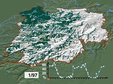
Paper from: Dusan Petrovic (Editor): ICA Proceedings of the 5th Mountain Cartography Workshop at
Bohinj, Slovenia, March, 29-April, 1, 2006, pp. 210-221.

classes can be predetermined: a much stricter control of the information flow compared for instance to the
individual’s preference during an exploration of a map display. The antagonism caused by a large spatial
coverage and a desired display in full resolution can be reduced, when a moving camera sequentially
portrays a landscape, however, at the expense of total spatial synopsis. Limited capabilities of static
media in documenting variations of two- or three-dimensional objects in time are the most apparent
reasons for animation. Thereby, a visual model obtains a spatial and a time scale.
Animation modes have been labelled after the dynamic component (GERSMEHL 1990):
- Stage-and-Actor Animation, where objects vary in visibility and graphic design in front of a static
   background,
- Model-and-Camera Animation, where viewing or illumination parameters change, and
- Metamorphotic Animation, where ever-present objects vary in shape and extent.
Depending on the role of time, we can further separate into temporal and non-temporal animation. If the
first makes use of forecast models or scenarios, we speak of a predictive animation. Furthermore,
animations can be structured by checking for realism. If real-world processes are utilised, the fraction of
observed or measured states (typically „key frames“ in a sequence) compared to simulated ones is crucial.

2.2 Animation and GIS Features
When relating animation methods to a GIS, several benefits become apparent:
A high thematic depth and a well-structured set of attributes are GIS features which inhibit simultaneous
presentation. To clearly separate between semantic and graphic attributes is a generally accepted rule,
which gives, on the other hand, flexibility in object selection and graphic symbolisation for each frame.
From imagery and terrain or surface models, flight-overs or walk-throughs with various degrees of
immersion can both be produced. A spatial overview can be achieved by watching a whole sequence,
whereas areas of highest interest can be positioned close to the optical axis of the virtual camera. Pictorial
(often from imagery) and abstract elements (for example from map data) might be used alternately or
simultaneously. Photorealistic and non-photorealistic presentations of spatial phenomena are functionally
complementary, and a simultaneous use can even serve the coding of specific attributes of geo-objects.
There is no geodata without implicit or explicit time reference. Analytical tasks might even specifically
rely on temporal change. Whenever ideas or formal models of the type, extent and distribution of
dynamics are missing, an animated visualisation provides the most efficient access to an exploration of
changes in terms of individual events and associated patterns. At the same time, animation can strongly
assist in finding outliers within data series, which might later on require a special treatment or
elimination. This sort of cognition, in return, encourages the development of new hypotheses and,
eventually, new process models. But even if a process model exists in advance, its results may be proved
against observations through animation.
A further advantage is the fact, that moving objects within someones field of view are a stronger
stimulant of visual perception than static ones.

3. The Dresden Altai-GIS
3.1 Objectives and Contents
The idea of animation should now be linked to the „Altai-GIS“. All general characteristics mentioned in
the last paragraphs are inherent: Spatial coverage is large. As an ecological GIS it stores themes of high
diversity (see Tab. 1). Data structures comprise vector layers, maps and image data from a multitude of
sensors (PRECHTEL 2003): Pictorial and abstract elements can thus be fed into an animation.
The GIS, in general, needs to lay-out an informative foundation for use in management of conservation.
Use might also contribute to the idea of eco-tourism (PRECHTEL & BUCHROITHNER 2002).
The GIS is set up in two levels: The focus level covers the Katun-Range in the Central Altai (about 8,500
km2); an overview level depicts the whole mountain system including its forelands (about 430,000 km2).
The Katun-Range part is termed „Altai 100“ to indicate a level of detail corresponding to a map scale of 1
: 100,000, while the so-called „Altai 1000“ data might have an equivalent scale of around 1 : 1,000,000.
A topic vector data listing is presented in Tab. 1. A more detailed discussion of contents, sources and
methodology might be taken from PRECHTEL (2003), or from the project homepage (PRECHTEL, 2005).
Paper from: Dusan Petrovic (Editor): ICA Proceedings of the 5th Mountain Cartography Workshop at
Bohinj, Slovenia, March, 29-April, 1, 2006, pp. 210-221.

                      Data Contents                                                       Data Level
                                                    ALTAI 100: Areal Coverage 49° 40' N –         ALTAI 1000: Areal Coverage 48° 00'
                                                    50° 20' N, 85° 30' E – 87° 00' E              N – 53° 00' N, 82° 00' E – 93° 00' E
         Category     Data Layer                    Data Type       Elements                      Data Type       Elements
                                                                    DHM100, DHM10,
                      Digital Elevation Models      Raster                                        Raster          DHM500, SRTM-3
                                                                    SRTM-3
                      Spot Elevations               Point                                         Point
         Relief
                      Gauge Elevations              Point                                         Point
                                                                                                                  elevation tints &
                      Hill Shading                  Raster          elevation tints & shading     Raster
                                                                                                                  shading
                      Relief Facets                 Polygon         type of neat lines            -------
                                                                    numerical shape
         Geomor-      Valley Shape                  Polygon
                                                                    parameters
         phology
                      Macro-Relief Types            -------                                       Polygon
                      Morphological Mountain Edge   -------                                       Polygon
                      Rivers                        Line                                          Line            Strahler Order
                      Streams                       Polygon                                       Polygon
                      Lakes                         Polygon                                       Polygon
         Drainage
                      Watersheds/Catchments         Polygon                                       Polygon
                      Late Pleistozene Meltwater
                                                    -------                                      Polygon
                      Lakes
                      Glacier and Perennial Snow    Polygon                                      Polygon
                                                                    glaciers of Belukha massif
         Cryosphere   Actual Glacier Fronts         Line                                         -------
                                                                    2001-2004
                      Ice Age Glacier Front         -------                                      Polygon
                                                    Raster,
                      Forest, General                                                            Polygon
                                                    Polygon
                                                    Raster,         deciduous, coniferous,
                      Forest, Classified                                                         -------
                                                    Polygon         mixed; krummholz
                      Meadows and Pastures,         Raster,
                                                                                                 Polygon
                      General                       Polygon
         Land Cover
                                                                    marshy meadow, dry
                      Meadows and Pastures,         Raster,         meadow, hill zone
                                                                                                 -------
                      Classified                    Polygon         meadow, alpine meadow,
                                                                    mountain tundra
                                                    Raster,
                      Void of Vegetation                            rock and scree               -------
                                                    Polygon
                      Settlements                   Polygon                                      Point           function, population
                      Streets                       Line                                         -------
         Settle-
         ments        Blocks                        Polygon                                      -------
                      Single Buildings,
                                                    Point                                        -------
                      Sheds and Shelters
                                                                    major road, minor road,                      major Road, minor
         Commu-       Roads and Pathes              Line                                         Line
                                                                    foot path                                    road, foot path
         nication
                      Railroads                     -------                                      Line
                      State Borders                 Line                                         Line
         Admini-
                      Administrative Borders                                                     Polygon
         stration
                      National Park Borders         Polygon                                      Polygon
                                                                                                                 Temperature and
                      Meteo-Stations                -------                                      Point
         Clima-                                                                                                  precipitation
         tology       Snow Cover Time Series        -------                                      Raster          1997, 1998
                      NDVI Time Series              -------                                      Raster          1997, 1998, 1999
                      Faults                        -------                                      Line
         Geology      Tectono-Stratigraphic Units   -------                                      Polygon
                      Ore Ressources                -------                                      Point
                      Conservation, General
         Facilities                                 Point                                        -------
                      Administration
         Docu-
                      Photo Points                  Point                                        -------
         mentation

        Tab. 1: Data of the Dresden Altai GIS (without imagery).

3.2 Contents Suiting Animated Presentation
Animations in particular suggest themselves for two reasons:
On the one hand material for temporal animation had already been prepared. A snow cover series of
„Altai 1000“ formed one strong base. A further time series of vegetation index observations (NDVI),
created in the same scale, has only recently been completed and should find entrance into the film soon.
Variations of glacier extents theoretically would provide another source. But low observation frequency
and a weak empirical data base for a prediction of the ice dynamics in-between observations inhibit an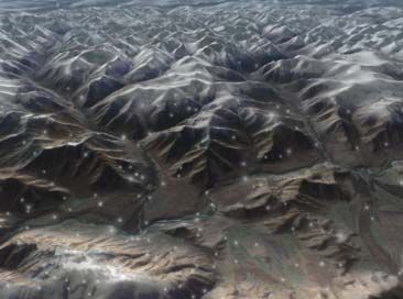
Paper from: Dusan Petrovic (Editor): ICA Proceedings of the 5th Mountain Cartography Workshop at
Bohinj, Slovenia, March, 29-April, 1, 2006, pp. 210-221.

animated model at present. Such a case of a long observation time (1962 until present) but a small number
of assured key frames might be displayed by a slide show technique.
On the other hand, virtual flights over the study area – a familiar type of non-temporal animations – are
also enabled by our data. These will incorporate DEMs and satellite imagery, classified land cover raster
or vector layers, respectively. This sort of animation can strongly promote the mental idea of the
landscape character.

4. Non-Temporal Animation – A Virtual Flight
4.1 Data for the Flight
Three-dimensional landscape visualisations consist of a geometry which emulates the shape of terrain,
and a texture overlay which contributes to complexity and visual realism of a scene (SUTER 1997). Two
raster DEMs with 500 m and 100 m cell spacing („DEM500“ and „DEM100“ of Tab. 1) were used as
principal geometry sources. Spot elevations, hydrological structure lines and lake polygons served as
ancillary data in securing relief consistency. Depending on camera height and field of view, different
levels of geometric detail could be produced and amalgamated. Thereafter, Landsat ETM winter and
summer scenes were processed to form the surface textures.

4.2 Pre-processing of the DEM
Standard GIS-software and image processing software (like Arc/Info and Erdas Imagine “Virtual GIS”)
store terrain surfaces by regular raster cells or irregular triangular networks (2.5-dimensionally), whereas
high-end animation software uses 3D vector formats (with rather strict limits to the maximum number of
meshes). Softimage|3D in the version 3.9.1 (an approved software 3D animation software for film
productions) was chosen for the production proper with a friendly assistance of the staff of the Dresden
University Computing Centre. Data transfer could be realised through the universal VRML code for web
applications.
An optimisation of the original relief models using standard software was the first task. It aimed at
maximum detail on the one hand and low complexity for storage and subsequent rendering in
Softimage|3D on the other. The Arc/Info TIN-format and associated functions for TIN handling fitted
best into these demands by allowing accuracy control and a limiting of the number of meshes. While the
existing DEMs constituted the bulk of data, the addition of point, line, and polygon coverages provided
further mass points, break lines and exclusion polygons. The resulting TINs adapt well to the highly
variable relief of the landscape.
Three different TINs were generated and exported for the virtual scenes. Two of them, derived from
„DEM500“, apply to the Altai Republic and have been tailored to the extent of a Landsat ETM mosaic of
66,000 km2. A third was based on the „DEM100“ for a low altitude flight and panoramic panning within
the inner study area of 8,500 km2. All produced TIN-data comprise of smaller triangles along the optical
axis of the camera and a slightly thinned fabric towards the margins.

4.3 Realisation of the Animation
After importing the geometry to Softimage|3D, edges between the triangular planes with angles below
60° were smoothed. For quicker handling, co-ordinates were then centered around the datum and all
elevation entries vertically exaggerated by 1.5 to strengthen the visual relief impression.
Landsat ETM bands 3,2, and 1 from two scenes (Aug., 17, 2001 and Oct., 15, 1999) were transferred to
Softimage|3D as RGB-TIFF data after small radiometric corrections for shadow zones and light haze.
Optical surface properties were set matt in order to avoid conflicts with the illumination at date and time
of image take. Additionally, a dome with a skylight-like brightness distribution and synthetic clouds was
designed around as a model atmosphere.
Flight animations deal with variation of observer position and view angle relative to a model landscape
and have been termed „Model-and-Camera Animation“ before. Key frames are defined by camera co-
ordinates and focus, whereas the motion is interpolated along a splined path for in-between frames.
Obviously, one makes sure that model edges are invisible, in order to establish a natural horizon. For the
main sequence covered by the two Landsat ETM scenes, an S–shaped path was defined, starting in the
North-East of the Altai Republic, and moving over medium-range mountains to the high mountains of the
South. A small camera icon simultaneously scans a sketch map at the display edge and helps to localise
the actually portrayed landscape.
Paper from: Dusan Petrovic (Editor): ICA Proceedings of the 5th Mountain Cartography Workshop at
Bohinj, Slovenia, March, 29-April, 1, 2006, pp. 210-221.

A second sequence showing a winter landscape works with the same type of data, but a fixed camera
position and a continuous turn of the camera through a panoramic pan. Falling snow in the foreground
was created with Softimage|Particle to thematically lead over to the film topic of snow cover change (fig.
1).
The animation was rendered with “mental ray 2.1” according to the PAL television standard.

Fig. 1: The virtual Altai during winterly snowfall.

5. Data of Snow and NDVI-Dynamics
5.1 Pre-selection of AVHRR-Data
Research on snow cover dynamics has initially been funded by a NATO Collaborative Linkage Grant.
We had picked a two-year observation period (1997/98) for the existence of high-resolution reference
imagery. This study has been based upon AVHRR-14 images. A temporal extension is already on the
way. In order to make additional use of the imagery, we later continued with a NDVI study, which
additionally incorporates AVHRR-16 images. Herein, the observation period has been extended (1997-
2002), but seasonally restricted to the months from March until October.
A pre-selection of a vast number of NOAA’s archived images is the first step. Suitable criteria were:
- Study area located within a 35° viewing cone (to limit resolution degradation and relief displacements),
- cloud coverage zero or low,
- high number of observations at the peak of snow dynamics (spring and autumn),
- frequent observations during the vegetation period for the NDVI dynamics.

5.2 Radiometric Preprocessing and Rectification
Sophisticated image applications need a conversion of greyvalues into physical measures. Data
calibration at data user’s side corrects for insolation, sensor degradation and thermal attenuation effects.
The planimetric accuracy of a geometric rectification using ephemeris data of the header files is in a
range of 0.05° - 0.1° (CRACKNELL 1997): substantial geometric improvement is needed to account for the
steep environmental gradients of a mountain area. A cloud-free summer scene with high radiometric
dynamics and a minimum snow has been identified as the master image. Its primary rectification by
ephimeris data has then been refined by manually positioned Ground Control Points (GCPs). The rectified
master scene then served as a uniform reference for image-to-image registration, a method that delivers
more homologue points than an image-to-map search. For a final geometric fine-tuning of all co-
registered scenes, an automated step was finally added. It compares image shorelines to reference
shorelines taken from maps, and iteratively produces a mutual best fit. A gradient descent method is
applied to the rastered reference model and serves for a global geometric rating (PRECHTEL &
BRINGMANN 1998).

5.3 Snow Classification and Interpolation under Clouds
Now the snow classification had to be carried out. Its principles are explained more in detail by HÖPPNER
& PRECHTEL (2002). A reference method has been developed at Bern Universty (VOIGT et al. 1999). The
authors describe a pixel-based, hierarchical method using spectral or bi-spectral thresholds. A basic set of
input values, derived from our own imagery and from exterior findings, gave an introduction point for a
raw classification, which had then to be evaluated. Thereafter if needed, threshold alterations were
applied until the results were in good accordance with a careful visual interpretation. Control aids for a
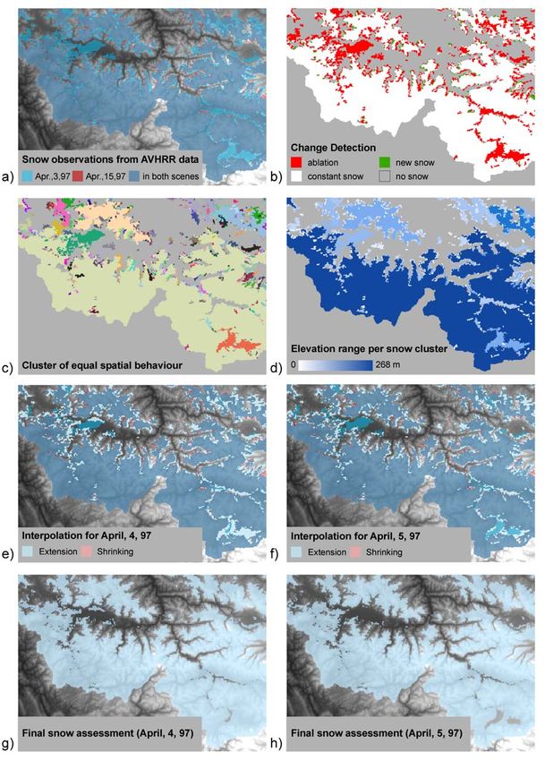
Paper from: Dusan Petrovic (Editor): ICA Proceedings of the 5th Mountain Cartography Workshop at
Bohinj, Slovenia, March, 29-April, 1, 2006, pp. 210-221.

tuning of the NDVI threshold and the reflectance limits of AVHRR-3 were given by: the „snow-
vegetation-view“ (AVHRR-1, NDVI and reflective part of AVHRR-3), and the „snow-cloud-view“
(AVHRR-1, AVHRR-2 and the reflective part of AVHRR-3). Besides a snow mask, a cloud mask was
generated, which leads over to the remaining problem of classification gaps under small cloud clusters.
Our solution assumes that the snow line is the best predictable measurand, when analysed per „Snow
Cover Unit“ (SCU), meaning a snow segmentation by terrain inclination and aspect. Stratified by SCUs,
all DEM cells bordering snow clusters of the classification have been triangulated. Then, all locations
above the predicted snow line within the no-data islands could be added to the snow class.
In the context of the animation, these „refined“ observations could now form key frames. But to arrive at
an evenly spaced time series, a methodology still required to be found which was, in the same time, both
simple and also close to the processes of snow accumulation and depletion. This demand excludes for
instance two-dimensional morphing operations.

5.4 From Unevenly Spaced to Daily Snow Assessments
The interpolation algorithm (comp. fig. 2) takes into account that the extent of snow mostly varies with
terrain altitude. Snow melt usually starts in the lowlands and valleys to gradually migrate uphill whereas
fresh snow cover begins to build up in higher elevation first to eventually migrate downhill. More
complicated climatic processes of a local scale had obviously to be disregarded in a large-area
presentation (100,000 km2).
Firstly, two consecutive AVHRR classifications were analysed for spatial differences (fig. 2a and 2b).
„Change of snow“ pixels were then clustered (using an 8-cell neighbourhood, fig. 2c). This makes it
possible to subdivide clusters of spatial increase or decrease into a number of evenly-spaced altitude
intervals (fig. 2d) and their member cells, respectively, which can sequentially be filled or freed of snow
according to the number of days between two consecutive observations (fig. 2e and 2f). However,
discontinuous precipitation behaviour (e.g. periods of stagnant snow cover, times of fast melting or
spreading of fresh snow) means that such a simulation appears rather unrealistic. Aiming for higher
realism meant incorporating supplementary meteorological data. Daily precipitation measurements in a
suitable spatial distribution were not available, and will not be available due to a lack of stations within
the vast uninhabitated parts of the Altai. But, alternatively, the „Northern Hemisphere Snow and Ice
Cover Chart“ by NOAA is a source that shows snow/ice extents on a daily base, even if aggregated to a
poor spatial cell resolution of around 25 x 25 km2. Therefore it cannot replace the original observations
(500 x 500 m2-cells), but appears to be useful in sharpening the dating of major snow dynamics, be it the
development of fresh snow cover or the retreat of snow. The key idea is its use as a temporal predictor of
variation. Some preparatory processing was required in order to advance its integration:
- conversion to binary snow mask
- projection change and vectorisation to harmonise with the “Altai 1000” GIS standards.
Now, the chart was toughened up to predict the temporal and – in a lower resolution – spatial behaviour
between two AVHRR observations. As a result, the altitude-dependent interpolation lost its schematic and
linear behaviour. Variation of each observed snow cluster could be initiated or terminated in a reaction to
the state shown in the „coarse“ daily Snow and Ice Cover Chart. The simulated snow fall and snow melt
now stagnates or speeds up like in reality. One “inescapable” restriction, however, should be named: The
algorithm only admits an one-directional process between two consecutive classifications - advance or
shrinkage of the snow extent -, and, vice-versa, cannot account for an oscillation, which was in some
cases indicated in the Snow and Ice Cover Chart. In spite of good co-relation between high- and low
resolution snow cover information from these independent sources, some contradictional patterns
emerged. The corresponding clusters thus failed to be treated in this standard manner. Dynamic clusters in
the AVHRR classification without indication in the Snow and Ice Cover Chart had to be processed
according to the simple linear altitude step principle explained above.
Following these rules, daily snow masks from January, 12, 1997 to December, 16, 1998 could be
produced. The few days from 1st of January, 1997 to the first observation day as well as the missing days
from the last observation to the end of 1998 were simply added by copies of the closest frame. This
should be a passable solution because of the small variation in high-winter snow.
Paper from: Dusan Petrovic (Editor): ICA Proceedings of the 5th Mountain Cartography Workshop at
Bohinj, Slovenia, March, 29-April, 1, 2006, pp. 210-221.

Fig. 2: Temporal densification from original snow observations to daily snow assessments.

5.5 NDVI Information from AVHRR-Data
The study of vegetation dynamics obviously has a close thematic link to the snow cover topic. For
example, a snow load retards the progression of the “green wave”, while snow melt can be a stimulus by
dispensing water. The main motivation to produce proprietary NDVI data instead of using archived
composites is their standard processing scheme which aggregates NDVI maxima within large spatial cells
Paper from: Dusan Petrovic (Editor): ICA Proceedings of the 5th Mountain Cartography Workshop at
Bohinj, Slovenia, March, 29-April, 1, 2006, pp. 210-221.

and inevitably “smears” the elevation-dependent small-scale variations, which make up the character of a
mountain landscape.
Since using the same AVHRR data, the geometric and radiometric treatment could follow the principles
given in the previous chapters. After a completion of all calibrations, the NDVI can be calculated using
the well-known formula of normalised differences between reflectance values of near-infrared and red.
However, a partial cloud cover within many selected scenes (associated with sudden NDVI drops)
produces the same sort of missing value problem as in the snow case. Snow and cloud masking was,
therefore, again necessary to exactly pinpoint data gaps and to convey cloud pixels to interpolation
algorithms. NDVI values of snow pixels, on the other hand, can either be treated like any other surface
information, or otherwise be flagged as a separate class.

5.6 NDVI-Assignment under Clouds
The development of an algorithm to realistically fill observation gaps under preservation of the full
geometric resolution is again demanding (conf. GROTEN & IMMERZEEL, 1999). Tests for improvements
are still under examination. REINHOLD (2004) has proposed and implemented a hierarchical processing
chain which makes use of temporally neighbouring scenes. Missing NDVI values are substituted by linear
interpolation along the time axis between neighbouring scenes. If this fails again due to further missing
values, he slots in an archive composite, but uses transformed (reduced) values. The necessary offsets are
determined by a comparison of valid NDVI values of the fragmentary scene and the associated
composite. An inherent problem of this method is the non-linear behaviour of the NDVI especially in the
initial and late phases of the “green-wave”. Further improvement seems feasible by additionally
considering existing land cover and DEM information. In an analogue approach to the snow cover units,
we can make use of the persistence of spatial patterns. In practice, we assume that the same land cover
type in similar elevation also shows similarities in the NDVI development, whereas the spatial correlation
decreases with increasing spatial distance.

5.7 From Unevenly Spaced to Daily NDVI Assessments
For merely practical reasons – multi-purpose use and a standardised calibration of primary data – only
NOAA data have so far been used. The inherent problems of longer periods of missing data could partly
be overcome by a future incorporation of further sensors like the SPOT vegetation instrument. Slightly
different NDVI responses due to a different technical layout of the NOAA- and the SPOT instruments
(red band SPOT-Vegetation/NOAA-16: 0.61-0.68 µm/0.58-0.68 µm, near infrared band SPOT-Vegeation/NOAA-16: 0.78-
0.89 µm/0.725-1.10 µm) have to be corrected by statistical methods, when using 10-day composites. A
reasonable spatial resolution of these composites (1 km × 1 km) and a 10-day frequency however strongly
promote a use. Thereafter, following the principal rules of the snow series (frame rate), daily NDVI
assessments could eventually be produced. In spite of the obvious deficiencies of linear interpolation,
only this simple way of densification seems realistic, because the relations between daily standard
observations of the meteorological stations (like temperature and precipitation) and the NDVI response
are pretty intricate.

6. From a Time Series to a Temporal Animation
6.1 Theory and Design
Considerations advancing a production of an animation refer to the character of spatio-temporal dynamics
to be displayed, and the underlying geodata: BLOK’s (2005) very systematic treatment classifies the
spatial behaviour of geo-objects into (dis-)appearance, mutation and movement (including or not
including change of shape), while complementary terms are moment (in the sense of an event time),
sequence, duration, pace and frequency for the temporal domain.
Object dynamics find an equivalent in BLOK’s system of dynamic visualisation variables. They reflect the
change of a graphic (composed of traditional static graphic variables) in time. The author identifies four
of them, and terms them moment of display, order, duration and frequency.
Such a framework spans a puzzling parameter space which is formed by combinations of object dynamics
– maps typically display several semantic elements in a synoptic way – and by likewise multiple modes of
their dynamic visualisation. Only a concentration on concrete tasks helps in arriving at a limited number
of sensible design options:
Paper from: Dusan Petrovic (Editor): ICA Proceedings of the 5th Mountain Cartography Workshop at
Bohinj, Slovenia, March, 29-April, 1, 2006, pp. 210-221.

Referring to the three principal modes of animation (chap. 2.2), we created Stage-and-Actor Animations:
the stage is the “stable” landscape portrayed by geometry and a basic texture; the actors are snow and
vegetation changing “on top of” the underlying texture.
Firstly, we consider the selection of GIS contents for our temporal animations, of which snow cover
extent and vegetation cycles (shown by NDVI-values) will be discussed. From a dominant relief
influence, patterns of our dynamic objects appear fine-grained, partly scattered, and, therefore, not easily
perceivable. Presentation design has to react by reducing the background information to a minimum
quantity of stable elements to be shown in a distribution which still provides an acceptable localisation.
The principal drainage network, border lines, and five major colour-coded land cover classes make up our
final selection.
Secondly, we must assist the comprehension of what are or what we assume to be dominant interrelations
between the theme (snow, NDVI) and its geographical environment. Herein, we start with a hypothesis at
hand and not with data mining in mind (meaning an explorative data analysis, which tests a focus data set
for the occurrence of a-priory unknown conspicuous signals and interrelations). In practice, we stress the
three-dimensional location, and, from the discussion of two-dimensional base map contents above, only
the relief is left for graphic coding. We decided for the creation of a rendered oblique view with constant
view direction and illumination (including a slight vertical exaggeration of the DEM). It is obvious that
the illumination as the prominent depth cue may not only affect the (topographic) background but also the
animated focus objects. Design options using relief derivatives like contour lines and spot elevations can
quickly be discarded (display space, perception time needed).
Thirdly, the theme of the animated sequence comes into the focus. Design may start with a single frame,
but cannot disregard the spatial variations over the whole sequence:
Snow cover is (in our study) a quality only changing from existence to non-existence and back. According
to BLOK’s (2005) scheme dynamic object features are appearance and movement through shape
metamorphosis. The graphic translation works as follows: where snow is present, it hides the background
land cover: a pixel changes from colour to white and back to colour when again becoming snow-free. We
can speak of a dynamic region mosaic which is using colour as graphic variable. The wintertime phases
of degraded spatial orientation, when snow screens much of the underlying land cover, can probably be
bridged since the observer can form his spatial knowledge during the summer phases of the sequence.
Things are quite different concerning the NDVI dynamics. A vegetation index - as an omni-present
quantitative parameter - undergoes a temporal change of value, whilst its spatial reference (a pixel)
remains constant (“mutation” in BLOK’s diction). It completely fills the model space and, hence, its
graphic representation cannot dynamically replace parts of a topographic background as in the snow case.
Borders and drainage network can be kept unaltered: they do not occupy much space, and, furthermore,
water bodies do not show much NDVI change anyway. An associative NDVI colour scale (from shades
of green through brown and yellow to grey) seems a logic graphic key. A stepped colour scale, a-priory
not a first choice, will be less ambiguous compared to a continuous one since the terrain illumination
additionally modulates the colours. Solutions for a smart joint display of the land cover patterns and the
NDVI values have, however, not been found: The combination of colour (NDVI) and simple
monochrome patterns (to show land cover) will fail due to the low display resolution. An alternative
assignment of contrasting hues to the land cover classes together with a saturation and intensity
modulation expressing NDVI states would strongly diminish the perceptibility of small alterations.
Splitting the screen into a topographic window and a thematic window causes a substantial degradation of
the spatial resolution. As a consequence, we propose the following procedure: Again we rely on dynamic
design options by inserting the topographic background into the NDVI sequence during the winterly
vegetation rest. This is the more self-evident as no NDVI observations have been carried out during
wintertime. The crucial mental link between NDVI dynamics and the geographic setting can be facilitated
by a careful trimming of the duration and frequency of these inserts (several breaks exist due to a multi-
year monitoring). Clear contrasts between NDVI and topography sections shall be able to avoid a mix of
information. Thereafter within repetitive runs, we plan to break up the animation into focus sequences:
NDVI variations for each individual land cover class can now pronounce exactly these interrelations. The
total sequence will hopefully foster a comprehensive understanding.
A last question relates to the transport of meta-information. In both models the primary information is
taken from satellite imagery. An uneven-spaced observation frequency is due to a varying cloud cover.
The production of frames in a frequency of one day or even higher using smart interpolation techniques
nevertheless coincides with a variable accuracy or reliability of the information shown. Our answer is to
add small markers indicating observation dates to the time diagram which generally serves as a temporal
orientation element.
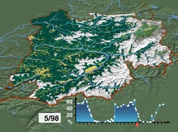
Paper from: Dusan Petrovic (Editor): ICA Proceedings of the 5th Mountain Cartography Workshop at
Bohinj, Slovenia, March, 29-April, 1, 2006, pp. 210-221.

6.2 Remarks on the Technical Realisation
The animation of the snow dynamics has fully been implemented (LONDERSHAUSEN 2004), while an
extension by the NDVI time series has so-far only been drafted.
The „DEM500“ geometry could be used as in the case of the flight animation. Synthetic land cover
textures created from „Altai 1000“ vector data (Tab. 1) serve as background for the presentation of
seasonal dynamics.
By comparison to the above, whilst the landscape state is changing, the virtual camera remains stable. It is
positioned in the south west and facing north east for a complete view of the Altai Republic. The land
cover determines the background texture and is superimposed by a varying snow texture. The original
730 masks had to be duplicated in order to reduce the animation speed to a more suitable pace for the
perceptive abilities of the spectator (58.4 seconds or 1460 frames). They are all treated as individual
frames, whereas „black“ pixels indicate transparency. Additional shading from an infinite light source
enhances the relations between relief and snow. A diagram in the lower right corner of the display
illustrates the temporal progression and dynamically informs about the actual percentage of snow covered
land. Technically, it becomes a second small animation over the same time range. Axes and graphs with
markers at each classification date (key frame) are stable, whilst the pointer and the filling below the
graph are following the snow cover frames (Fig. 3 and 4).

Fig. 3: Frame showing high-winter snow cover                  Fig. 4: Frame showing a situation during snow melt
(January, 1997)                                               (May, 1998).

7. Outlook
The film clearly shows advantages of dynamic geodata presentation. The major target was to broadly
inform an interested public on the landscape character and the specific project results. Speaking of results
implicates, that the methods applied were chosen for a best possible transfer of evaluated information
(without claiming to have an explanation for every detail shown). A more explorative use of the data by
means of animation certainly bears a further strong potential, but was not intended in the first instance.
Some principal deficiencies, within the process from concept to technical realisation, motivate further
research and can be grouped into the categories:
- theory of visual communication,
- display techniques, and
- production techniques.
Referring to communication theory, BLOK (2005) reports on key issues associated to a temporal
animation of geodata: A well balanced number of visual stimuli is crucial for avoiding “change
blindness” and “inattentional blindness”. Closely related to the latter, “figure-ground perception” must be
smartly supported for a best-possible knowledge extraction; a user only benefits if he will be able to
separate characteristic patterns (“figures”) from a background (“ground”). Characteristic means, within
this context, that the patterns can actually be recognised and typified due to simple geometric shape or
due to obvious relations to a-priory known geo-features (like a valley, a certain elevation level, a
settlement, etc.). Especially if an animation is a fixed product offering only the standard interaction
modes of the media player, one would strongly profit from better guidance on the limits of visual
comprehension in relation to complexity of visual geo-information within a dynamic sequence.
Many potential problems are inherent within the snow cover sequence: patterns of various size change in
different relative positions and velocities. The dynamic time scale also has to be kept in view. At the same
time, the presentation speed has to react on the given temporal resolution of the model in order to show
Paper from: Dusan Petrovic (Editor): ICA Proceedings of the 5th Mountain Cartography Workshop at
Bohinj, Slovenia, March, 29-April, 1, 2006, pp. 210-221.

smooth motion (see 2.1). As a result, an eventually overstrained user may only react by repeating a whole
sequence or by stopping it at points he wishes to focus upon. It is noted that the postulation of a smooth
motion is – within a certain range – task-dependent, and might justifiably be given up for an exploration
of individual states and patterns in a strongly reduced speed. Additionally, a sound track might have
alternatively been used for the time relation in order to simplify the visual canal.
This leads over to display techniques. Standard control functions of for instance a DVD player are
limited. Flexible zoom, speed alterations, and cuemarks would give higher flexibility, especially for work
with educational or scientific material. As a low-effort response to the problem, we created an initial
selection menu which already allows the starting of predefined sequences by a mouse click.
Geodata display on electronic devices brings a lot more difficulties: a small display area with limited
resolution, and device-dependent colour reproduction are obvious problems. Less known is the
impossibility to equally fulfil the display requirements of both a computer monitor and a TV set (MÄUSL
1995). The latter not only suffers from even lower resolution compared to PC monitors, but also an
uneven side-ratio of the pixels. Computer-generated frames of 768 by 576 pixels have to be resampled to
720 by 576 pixels to show correct dimensions when displayed on a television. An “image cash” of 20 to
40 pixels further reduces the visible image parts. Alternating “writing cycles” between even and odd lines
of the image matrix in a frequency of 50 Hz (PAL standard) cause flickering along horizontal lines with
static image signals. This is clearly less of a problem for filmed sequences but more noticable in
animations with a static camera.
Production techniques. Quite an efficient automated data flow from GIS-stored geodata to an animation
software has already been achieved, but further improvements could both smooth it and speed it up.
Examples can be given: for use in animations, the level of detail (LOD) of a DEM should react to camera
perspectives; larger tolerances compared to a full-resolution DEM are allowed with increasing distance to
the camera. Built-in LOD steering, of software at hand, performed unsatisfactorily. A “work-around”
using TINs with terrain-adapted tolerances (and mesh densities) therefore became necessary. Cutting-
lines parallel to the flight path were then generated, and, finally, a new TIN mosaic was assembled. A
smarter solution would allow DEM thinning within one step, using a distance-dependent elevation
tolerance function. Texture handling could also be improved. If texture means a colour-coded area
mosaic, the work-flow is quite simple: tabular data, for instance, relates polygon attributes of a coverage
to codes, which will then become cell values of a raster representation with size and resolution both set to
the animation standards. A further table can now connect the cell values to the desired colour scheme, and
the RGB-image matrix can be exported using a supported format. However, if object properties are
displayed by complex textures (e.g. a forest by individual trees) or with dynamic visual attributes, no
smooth interface exists to the “animation world”. If dynamic legends are produced, some user interaction
is also required. As stated above, these are handled as independent sequences in the software, and, only
within a second step, become fused with the other image contents.
This article could only select a few aspects from a wide field of potential further research. Effort in
improving dynamic geodata presentations will be fully justified. Limitations by hardware performance,
software functionality and data availability are currently small and will further decrease in future.

8. References
BLOK, C., 2005: Dynamic Visualization Variables in Animation to Support Monitoring of Spatial
Phenomena. - Netherlands Geographical Studies 328, Utrecht/Enschede, 190 p.
CRACKNELL, A. P., 1997: The Advanced Very High Resolution Radiometer. Taylor & Francis, London.
DRANSCH, D., 1997: Computer-Animation in der Kartographie. Theorie und Praxis. – Springer,
Berlin/Heidelberg.
DRANSCH, D., 2002: Term „Animation“ – in: BOLLMANN, J. & KOCH, .-G. (Hrsg.): Lexikon der
Kartographie und Geomatik, Spektrum Akademischer Verlag, Heidelberg/Berlin.
GERSMEHL, P.J., 1990: Choosing Tools: Nine Metaphors of Four-Dimensional Cartography. Cartographic
Perspectives, 5: 3-17.
GROTEN, S. & W. IMMERZEEL, 1999: Monitoring of Crops, Rangelands and Food Security at National
Level. A Tutorial for Individual and Group Studies. Enschede, the Netherlands: Department of
Agriculture, Conservation and Environment, ITC.
HÖPPNER, E. & PRECHTEL, N., 2002: Snow Cover Mapping with NOAA-AVHRR Images in the Scope of
an Environmental GIS Project for the Russian Altai (South Siberia). - Proc. of the ICA Comm. on
Paper from: Dusan Petrovic (Editor): ICA Proceedings of the 5th Mountain Cartography Workshop at
Bohinj, Slovenia, March, 29-April, 1, 2006, pp. 210-221.

Mountain Cartography, Mt. Hood, Oregon, May, 15-19, 2002, http://www.karto.ethz.ch/ica-
cmc/mt_hood/proceedings.html: 26 p.
LONDERSHAUSEN, K., 2004: Erstellung einer animierten kartographischen Präsentation von und aus
Inhalten eines komplexen Geoinformationssystems im Kontext der Dresdener Altaiforschung. – Diploma
Thesis, Inst. f. Cartography, Dresden Univ. of Techn.: 112 p.
MÄUSL, R., 1995: Fernsehtechnik: Übertragungsverfahren für Bild, Ton und Daten. – Hüthig, Heidelberg.
PRECHTEL, N. & BRINGMANN, O., 1998: Near-Real-Time Road Extraction from Satellite Images Using
Vector Reference Data. - Intern. Arch. of Photogrammetry and Remote Sensing, XXXII, 2: 229-234.
PRECHTEL, N. & BUCHROITHNER, M. F., 2002: The Contribution of Remote Sensing to Alpine Tourism in
Protected Landscapes. The Example of the Altai Mountains. - Grazer Schriften der Geographie und
Raumforschung, 37: 15-34.
PRECHTEL, N., 2003: GIS-Aufbau für den Naturschutz im Russischen Altai. - Geoinformationssysteme –
Theorie, Anwendungen, Problemlösungen, Kartographische Bausteine, 21: 82–100.
PRECHTEL, N., 2005: Geodatenerhebung, GIS-Aufbau und Kartenerstellung für den Katun-Nationalpark,
Altai-Gebirge (Sibirien) – Project homepage in German and English:
http://141.30.139.182/researchProjects/Altai/.
PRECHTEL, N. & LONDERSHAUSEN, K., 2005: Animating Geodata – Exemplified by the Dresden Altai-
GIS. Photogrammetrie – Fernerkundung – Geoinformation, 1/2005: 37-46.
REINHOLD, M., 2004: Erstellung einer NDVI-Reihe für die Republik Altai basierend auf
meteorologischen Fernerkundungsdaten (AVHRR). Seminar Thesis, Inst. f. Cartography, Dresden Univ.
of Techn.: 60 p.
SUTER, M., 1997: Aspekte der interaktiven Real-Time 3D-Landschaftsvisualisierung. – Dissertation,
Philos. Faculty II of Zürich Univ.
VOIGT, S., KOCH, M. & BAUMGARTNER, M. F., 1999: A Multichannel Threshold Technique for NOAA
AVHRR Data to Monitor the Extent of Snow Cover in the Swiss Alps. - Interactions Between the
Cryosphere and Greenhouse. Proc. of IUGG 99 Symposium, Birmingham, IAHS Publications, 256: 35–
43.

Addresses of the authors:
Dr. NIKOLAS PRECHTEL
Institut für Kartographie, TU Dresden,
Helmholtzstr. 10, 01069 Dresden
email: Nikolas.Prechtel@tu-dresden.de
Dipl.-Ing. KATJA LONDERSHAUSEN
INTEND Geoinformatik GmbH
Ludwig-Erhard-Straße 12, 34131 Kassel
email: londershausen@intend.de

Manuscript submitted: February, 2006
You can also read