Pressure and inertia sensing drifters for glacial hydrology flow path measurements - The Cryosphere
←
→
Page content transcription
If your browser does not render page correctly, please read the page content below
The Cryosphere, 14, 1009–1023, 2020
https://doi.org/10.5194/tc-14-1009-2020
© Author(s) 2020. This work is distributed under
the Creative Commons Attribution 4.0 License.

Pressure and inertia sensing drifters for glacial
hydrology flow path measurements
Andreas Alexander1,2 , Maarja Kruusmaa3,4 , Jeffrey A. Tuhtan3 , Andrew J. Hodson2,5 , Thomas V. Schuler1,6 , and
Andreas Kääb1
1 Department  of Geosciences, University of Oslo, 0316 Oslo, Norway
2 Department  of Arctic Geology, The University Centre in Svalbard, 9171 Longyearbyen, Norway
3 Centre for Biorobotics, Tallinn University of Technology, 12618 Tallinn, Estonia
4 Centre for Autonomous Marine Operations and Systems, Norwegian University of Science and Technology,

7491 Trondheim, Norway
5 Department of Environmental Sciences, Western Norway University of Applied Sciences, 6856 Sogndal, Norway
6 Department of Arctic Geophysics, The University Centre in Svalbard, 9171 Longyearbyen, Norway

Correspondence: Andreas Alexander (andreas.alexander@geo.uio.no)

Received: 1 June 2019 – Discussion started: 8 July 2019
Revised: 9 February 2020 – Accepted: 12 February 2020 – Published: 17 March 2020

Abstract. Glacial hydrology plays an important role in          averaged mean along the flow path. Furthermore, our re-
the control of glacier dynamics, of sediment transport,         sults indicate that prominent shapes in the sensor records
and of fjord and proglacial ecosystems. Surface meltwa-         are likely to be linked to variations in channel morphology
ter drains through glaciers via supraglacial, englacial and     and the associated flow field. Our results show that multi-
subglacial systems. Due to challenging field conditions, the    modal drifters can be a useful tool for field measurements
processes driving surface processes in glacial hydrology re-    inside supraglacial channels. Future deployments of drifters
main sparsely studied. Recently, sensing drifters have shown    into englacial and subglacial channels promise new opportu-
promise in river, coastal and oceanographic studies. How-       nities for determining hydraulic and morphologic conditions
ever, practical experience with drifters in glacial hydrology   from repeated measurements of such inaccessible environ-
remains limited. Before drifters can be used as general tools   ments.
in glacial studies, it is necessary to quantify the variabil-
ity of their measurements. To address this, we conducted
repeated field experiments in a 450 m long supraglacial
channel with small cylindrical drifters equipped with pres-     1   Introduction
sure, magnetometer, acceleration and rotation rate sensors
and compared the results. The experiments (n = 55) in the       Glacial hydrology plays a key role in glacier dynamics
supraglacial channel show that the pressure sensors con-        (Flowers, 2018), sediment transport and its impact on fjord
sistently yielded the most accurate data, where values re-      and proglacial ecosystems (e.g., Swift et al., 2005; Meire
mained within ±0.11 % of the total pressure time-averaged       et al., 2017; Urbanski et al., 2017). Surface water is gen-
mean (95 % confidence interval). Magnetometer readings          erally routed supraglacially, i.e., along the glacier surface
also exhibited low variability across deployments, maintain-    in ice-walled drainage systems. Water enters the englacial
ing readings within ±2.45 % of the time-averaged mean of        and subglacial drainage system through moulins, crevasses
the magnetometer magnitudes. Linear acceleration measure-       and cut-and-closure systems (Gulley et al., 2009). Ice-walled
ments were found to have a substantially higher variabil-       drainage systems have highly variable geometry, controlled
ity of ±34.4 % of the time-averaged mean magnitude, and         by the counteracting mechanisms of melt enlargement due to
the calculated speeds remained within ±24.5 % of the time-      dissipation of potential energy and creep closure of the vis-
                                                                cous ice (Röthlisberger, 1972). The capacity of the glacial

Published by Copernicus Publications on behalf of the European Geosciences Union.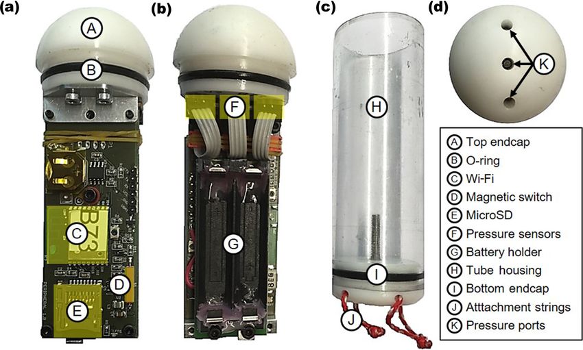
1010                                                                 A. Alexander et al.: Pressure and inertia sensing drifters

drainage system varies in both space and time and dynami-            (e.g., Boydstun et al., 2015; Xanthidis et al., 2016). Drifters
cally adjusts to the highly variable meltwater supply (Schoof,       remain the most promising method for the study of physical
2010; Bartholomew et al., 2012). These geometric adjust-             parameters along multiple flow paths within the hydrological
ments often form step-pool sequences (e.g., Vatne and Irvine-        system of a glacier. This is because Lagrangian drifters can
Fynn, 2016) and are responsible for up to 90 % of the total          be equipped with multiple sensors to collect data along the
flow resistance (Curran and Wohl, 2003). The channel geom-           flow path within the changing environment. Therefore they
etry influences flow resistance and water velocity (Germain          provide a wider range of observational data with reduced de-
and Moorman, 2016). Vice versa, the velocity controls the in-        ployment effort when compared to conventional fixed station
cision rates in ice-walled channels in conjunction with water        hydrological measurements.
temperature and the rate of heat loss at channel boundaries             Development of sensing drifters in glaciology has been
(Lock, 1990; Isenko et al., 2005; Jarosch and Gudmunds-              previously reported, most notably the Moulin Explorer by
son, 2012). Despite these findings, major knowledge gaps             Behar et al. (2009), which was unfortunately lost during its
remain, especially within subglacial hydrology due to lim-           first deployment. A successful glacial drifter was the elec-
ited observations of the environment. Specifically, the mech-        tronic tracer (E-tracer), as reported by Bagshaw et al. (2012).
anisms driving water routing from the glacier surface to the         The device has the size of a table tennis ball and included a
bed remain largely unexplored. Improving our understand-             radio transmitter to enable identification and data transmis-
ing of glacial hydrology and its effect on glacier dynamics          sion after passage through the subglacial system of Leverett
requires new methods. The methods should be able to pro-             Glacier, Greenland (Bagshaw et al., 2012). These encourag-
vide direct measurements of water routing on, through, and           ing results lead to a second generation of E-tracers equipped
under glaciers including the water temperature, velocity, and        with a pressure sensor and successfully transmitted pres-
pressure as well as the channel morphology along multiple            sure data from subglacial channels through 100 m of overly-
flow paths.                                                          ing ice after having been deployed in crevasses and moulins
   Direct measurements are the most ideal source of infor-           (Bagshaw et al., 2014). The published data remain sparse and
mation but remain scarce in glacial hydrology because they           limited to a single mean pressure record in Bagshaw et al.
are difficult to obtain (e.g., Gleason et al., 2016). Begin-         (2014). As with all new field measurement technologies, the
ning in the early 2000s, new technologies have emerged,              repeatability of in situ measurements is often very challeng-
and current methods for in situ tests include among others           ing to determine. Encouraged by the previous drifter stud-
Doppler current profiling in supraglacial systems (e.g., Glea-       ies by Bagshaw et al. (2012, 2014) with a single pressure
son et al., 2016), dye tracing (e.g., Seaberg et al., 1988; Willis   sensor, the present study explores the potential of sensing
et al., 1990; Fountain, 1993; Nienow et al., 1998; Hasnain           drifters with several different sensors (multimodal) to record
et al., 2001; Schuler and Fischer, 2009), salt injection gaug-       data along the flow path of glacier channels. The focus of
ing (e.g., Willis et al., 2012), geophysical methods (e.g., Diez     this work is to assess the repeatability of Lagrangian drifter
et al., 2019) and gas tracing (e.g., Chandler et al., 2013).         measurements in a supraglacial channel. Current methods,
   Lagrangian drifters are small floating devices, which pas-        such as dye tracing, allow for the repeatable measurement
sively follow the water flow and are commonly used to study          of the flow velocities averaged over the duration of a pas-
flow in large rivers, lakes and oceans. Most typically, drifters     sage. However, it is impossible to deconvolve these records
provide information about their position and speed (Lan-             to obtain spatially and temporally distributed information.
don et al., 2014). Depending on sensor payload, drifters can         The present study therefore also assesses the potential of
be used for a wide range of applications, including coastal          sensing drifters to acquire spatial and temporal variation of
and ocean surface current monitoring (Boydstun et al., 2015;         the velocity along a flow path. Furthermore, the multimodal
Jaffe et al., 2017) to estimate river bathymetry and surface         sensor data are investigated for potential time series features
velocities (Landon et al., 2014; Almeida et al., 2017) and to        that may be associated with geometrical features of the in-
collect imagery for underwater photogrammetry (Boydstun              vestigated supraglacial channel.
et al., 2015). Recent payloads in river studies included sen-           The experiments were carried out using a submersible
sors for temperature (e.g., Tinka et al., 2013; Oroza et al.,        multimodal drifter platform measuring at 100 Hz. The
2013; Allegretti, 2014), dissolved oxygen (e.g., D’Este et al.,      rugged, autonomous sensing platform records the water pres-
2012; Tinka et al., 2013), pH (e.g., Tinka et al., 2013; Arai        sure, as well as three components each of linear accelera-
et al., 2014), turbidity (e.g., Marchant et al., 2015), GPS          tion, rotation rate and the magnetic field strength. Repeated
receivers (e.g., Stockdale et al., 2008; Tinka et al., 2013),        deployments were carried out along a single section of a
acoustic Doppler current profilers (e.g., Tinka et al., 2009;        supraglacial meltwater channel (n = 55). The general ap-
Postacchini et al., 2016) and inertial measurement units (e.g.,      plicability of the cylindrical drifter is field tested, and the
Arai et al., 2014). Additionally, sensor payloads in oceano-         repeatability of the sensor time series is determined. Fi-
graphic applications included devices for the measurement of         nally, we investigate the potential of the proposed multi-
conductivity (e.g., Reverdin et al., 2010; Jaffe et al., 2017),      modal drifter to measure the surface transport velocity along
chlorophyll (e.g., Jaffe et al., 2017) and underwater imagery        a supraglacial channel flow path, and we critically assess the

The Cryosphere, 14, 1009–1023, 2020                                                      www.the-cryosphere.net/14/1009/2020/
A. Alexander et al.: Pressure and inertia sensing drifters 1011
device’s performance for glaciological applications. The de-
ployment in supraglacial channels allowed the study of the
sensor performance in a controlled environment. This is an
important step in the development of a reliable measurement
platform for supraglacial, englacial and subglacial studies.
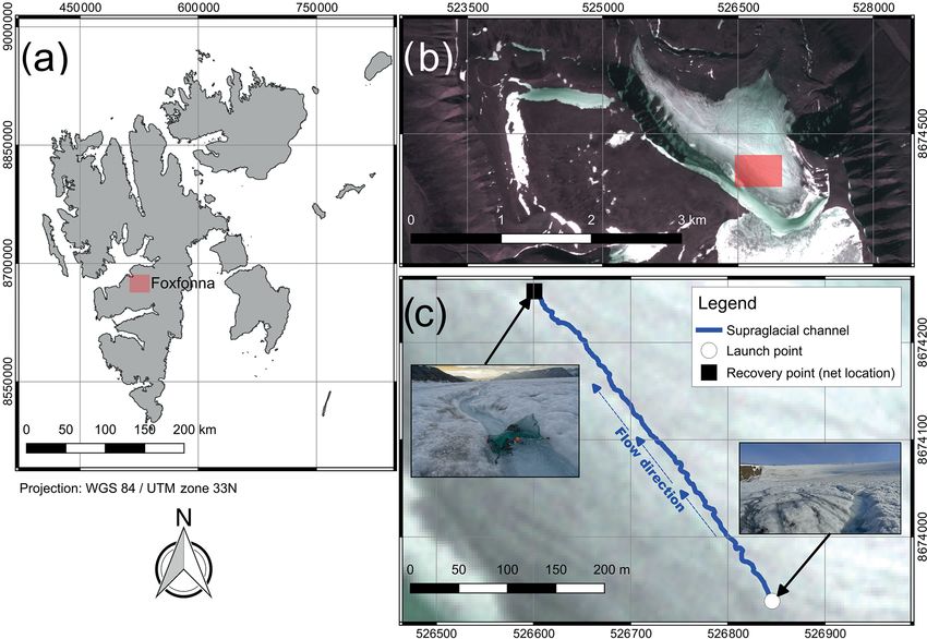
Figure 1. Dimensions of the multimodal drifter used in this work.
2 Methods The drifter includes three identical pressure transducers as well as a
single inertial measurement unit (IMU). (a) Side view of the drifter.
2.1 Multimodal drifter (b) Top view facing the cap showing the left (L), middle (M) and
right (R) pressure ports. (c) Body-oriented drifter coordinate system
The drifter platform used in this study has two custom- including the roll (φ), pitch (θ ) and yaw (ψ) angles.
machined polyoxymethylene (POM) plastic endcaps and a
4 cm outer diameter polycarbonate plastic tube. The device
has a total length of 12 cm and mass of 143 g. Neutral buoy- postprocessing. The drifter units use three pressure sensors
ancy of the drifter is achieved by manually adjusting the (marked as left, middle and right in Fig. 1) and can be out-
length of the sensor by screwing the flat endcap inwards fitted with either 2 bar or 30 bar sensors. The drifters were
or outwards to increase or decrease the total volume. Small designed this way to include triple modular redundancy by
balloons can additionally be attached to the drifter, to fine- including a pressure sensor array in lieu of a single pressure
tune the buoyancy in the field, and were used during the sensor. The middle pressure sensor (30 bar sensor) was how-
field deployment of this study. Each hemispherical endcap ever not used in this study due to the lower sensitivity and
of the drifters contains three identical digital total pressure range of pressures experienced during channel passage. All
transducers. When the device is submerged in flowing water, following work will therefore only refer to the two lateral
the total pressure is the sum of the atmospheric, hydrostatic (left and right, 2 bar) pressure sensors.
and hydrodynamic pressures. The devices are designed for In addition to the three pressure transducers, the drifter
a maximum pressure of 2 bar (MS5837-2BA, TE Connectiv- platform also contains a digital 9 degrees of freedom (DOFs)
ity, Switzerland) and a sensitivity of 0.02 mbar (0.2 mm wa- inertial measurement unit (IMU) (BNO055, Bosch Sen-
ter column). The pressure sensor data were recorded with a sortec, Germany) integrating linear accelerometer, gyroscope
resolution of 0.01 mbar. The accuracy of the pressure trans- and magnetometer sensors. The device uses proprietary
ducers was found to be 1 mbar. This was determined by test- (Bosch Sensortec) sensor fusion algorithms to combine the
ing fully assembled drifters in a laboratory barochamber up linear accelerometer, gyroscope and magnetometer readings
to an equivalent of 55 m of water depth, which is 2.75 times into the body-oriented Euler angles to provide real-time ab-
larger than the maximum rated pressure of the sensor. There- solute orientation at 100 Hz. These IMU sensors were chosen
fore, the main limitation of the drifter platform results from as they represent the current state of the art in IMU technol-
the measurement range of the chosen pressure sensors rather ogy. Additionally, they have the further benefit that the real-
than the ability of the mechanical components. Each pressure time calibration status of each of the three sensors is recorded
transducer is equipped with its own on-chip temperature sen- (0, lowest, to 3, highest) as part of each dataset in order to
sor, allowing for all pressure readings to include real-time provide quality control information for all IMU measurement
temperature correction using a two-stage correction algo- data. When running in sensor fusion mode, all variables are
rithm. The algorithm first takes into account device-specific saved at 100 Hz, with the exception of the magnetometer,
correction coefficients, specified by the manufacturer. In a which is recorded at a maximum rate of 20 Hz. The sensor
second step, the device’s temperature is used to output the fusion mode of the BNO055 has the major benefit that the
corrected total pressure reading depending on the tempera- absolute orientation, consisting of roll, pitch and yaw angles,
ture range. The algorithm is provided on page 7 of the man- is calculated in real time. The major downside is however
ufacturer’s data sheet (TE connectivity sensors, 2017). that the calibration and sensor fusion used in this procedure
All drifters are programmed for atmospheric autocalibra- are a black box, as Bosch has not released the algorithms.
tion. Once the device is activated using a magnetic switch, Previous studies in highly dynamic environments report the
data from each pressure transducer are logged for 15 s. The measurement error of the BNO055 in the pitch and yaw an-
atmospheric pressure, including any sensor-specific offset, gles for rapid body movements during driving as less than
is recorded internally. Afterwards, all three transducers are 0.4◦ and less than 2◦ for the roll angle (Zhao et al., 2017).
set to a default value of 100 kPa (1 bar) at local atmosphere. Similar results were observed for a series of static and dy-
All sensors are therefore autocalibrated to local changes in namic tests using a hexahedron turntable with the BNO055,
atmospheric pressure which occur during the day, directly where the error ranged from 0.53 to 0.86◦ for pitch angles,
before each field deployment. This feature removes the ne- 1.28 to 3.53◦ for yaw angles and 0.44 to 1.41◦ for the roll
cessity of manually correcting pressure sensor readings in angle (Lin et al., 2017).
www.the-cryosphere.net/14/1009/2020/ The Cryosphere, 14, 1009–1023, 2020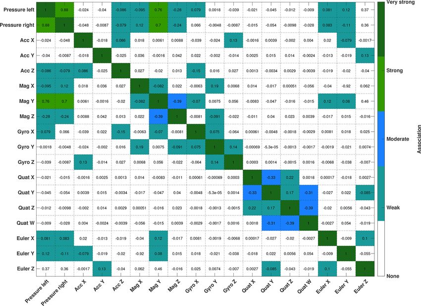
1012                                                               A. Alexander et al.: Pressure and inertia sensing drifters

   The drifters use the STM32L496 microcontroller unit             and being recovered. This involved deploying five wooden
(MCU). They are programmed with the STM32CubeMX                    drifter surrogates identical in size to our multimodal drifters
software in DFU mode over a USB full-speed interface. A            in a 2.5 km long supraglacial, partly englacial channel. The
ESP8266 Wi-Fi module is used for communication and con-            channel on the eastern side of the glacier had several well-
nected to the MCU via USART2. The IMU and pressure sen-            developed step-pool sequences and was incised deeply into
sors are connected via an I2 C interface and communicate via       the glacial ice. Further downstream, the channel developed
the I2 C protocol. The data are stored as a delimited text file    into a partially snow plugged, partially englacial system. The
at 100 or 250 Hz directly to a 6 or 16 GB microSD card. The        final channel section had a large amount of rock debris typ-
IMUs were configured to read out more data in addition to          ical of subglacial environments. A net was installed where
the dynamic linear acceleration (body acceleration due to ex-      the channel reemerged on the surface at the eastern lateral
ternal forcing only, gravity vector removed) and rate of an-       moraine. Emerging wooden sensor surrogates were trapped
gular rotation (rate gyro), relative to the x, y and z axes of     in the net and recovered by removing them by hand.
the sensor, as shown in Fig. 1. The additional data include           The second, main experiment was conducted along a
the real-time calculation of the drifter body orientation (3D      450 m section of a supraglacial channel on Foxfonna. The
Euler angles relative to x, y, and z axes and the angles as        investigated section had a total elevation difference of 30 m
quaternions) as well as the 3D magnetic field vector. The          (handheld GPS accuracy of 5 m) as measured between the
orientation of the vector measurements of the magnetome-           start and the end of the channel section. The section included
ter readings corresponds to the axes of the sensor which are       several step-pool sequences as well as rapids and recircu-
identical to the accelerometer and rate gyro axes. All drifter     lation zones. The experiments were conducted within this
sensor data are saved as a 27 column ASCII text file. The          channel section for three main reasons. First, the purpose of
text files were transferred from the drifters via Wi-Fi to a       the study was to determine field measurement repeatability,
field computer after drifter recovery from the stream.             requiring a channel with different morphological features.
   Vibration and destructive testing of the IMU and the drifter    Second, with only five prototypes, the risk of losing a drifter
housing have been conducted up to 3000 times the gravita-          had to be kept low. Finally, the study of the supraglacial sys-
tional acceleration, thus showing that the drifter platform can    tem allowed for the filming of deployments, and this provides
withstand high impacts. Deployment under harsh conditions          a simple and robust evaluation method to compare the sensor
was successfully proven during measurements inside large-          data with observed movements of the drifter within the flow.
scale hydropower turbines (Kriewitz-Byun et al., 2018). Dur-       All five drifters were launched from the location, marked
ing this study the drifter was only tested in supraglacial         with a white circle on the map in Fig. 3, and were recovered
streams. Subglacial deployments have however been suc-             using a marine fishing net, installed at the downstream end
cessfully conducted during subsequent field tests in 2019 and      of the channel section. A total of 55 drifter deployments with
will be described and analyzed in a later study.                   five individual multimodal drifters were conducted. A total of
                                                                   10 deployments were collected in the afternoon of the second
2.2    Study site                                                  field day (5 August 2019, 15:52–17:20 local time) and the re-
                                                                   maining 45 deployments in the late evening and night of the
Fieldwork for this study was conducted on the main island          fourth field day (7 August 2019, 18:53–23:37 local time).
of the Norwegian Arctic archipelago Svalbard between the           The discharge varied throughout the deployment time, de-
4 and 7 August 2018 on the approximately 5 km2 big val-            pending largely on weather conditions (sunny, with increased
ley glacier Foxfonna. The cold-based, roughly 2.9 km long          melt on 5 August, and cloudy, rainy and sunny on 7 August).
glacier is located on a northwest-facing slope between 330         The exact discharge was not recorded. Some of the deploy-
and 750 m elevation above sea level at the end of the Advent-      ments had slightly varying buoyancy, due to varying balloon
dalen valley, next to the main settlement Longyearbyen. The        inflation, but all deployments on the 450 m section were con-
glacier has a network of supraglacial channels developing on       ducted with a single balloon. Four out of the 55 deployments
the surface of the glacier during the summer ablation period.      had the drifters connected in tandem with cable ties to test
Some of the channels cut deep enough to form englacial cut-        the variation between the sensor readings of two different
and-closure systems (Gulley et al., 2009), and others remain       drifters passing through nearly identical flow paths. All of
partially snow plugged during the summer. Additional chan-         the drifters were switched on and then left on the ground for
nels emerge at the glacier front, indicating existing subglacial   at least 30 s before deployment and for an additional 30 s af-
drainage channels.                                                 ter successful recovery from the stream and before switch-
                                                                   ing off. This was done to ensure that the drifters had enough
2.3    Field deployments                                           time for self-calibration to atmospheric pressure before the
                                                                   deployment and the IMU sensor readings could calibrate and
Two different experiments were conducted on the glacier sur-       provide constant-value readings, which later serve to mark
face. The first experiment tested the general feasibility of       the start and stop of each deployment.
the drifters traveling through an englacial–subglacial system

The Cryosphere, 14, 1009–1023, 2020                                                    www.the-cryosphere.net/14/1009/2020/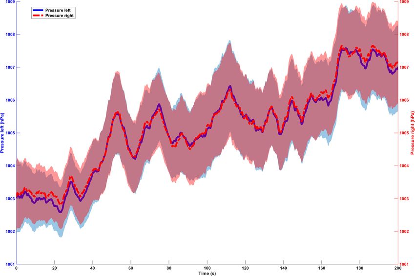
A. Alexander et al.: Pressure and inertia sensing drifters                                                                               1013

Figure 2. Detailed breakdown of the drifter. (a) Side view showing the drifter electronics. (b) Side view showing the reverse side of the
electronics board including the battery holder and pressure sensors. (c) Polycarbonate tube housing of the drifters with attachment strings for
balloons used for manual buoyancy adjustment. (d) Top view facing the cap, showing the ports for each of the three pressure sensors.

2.4   Data preparation and processing workflow

All data processing was performed using MATLAB R2018b.
Corrupted datasets with missing data or faulty sensor read-                                 number of recovered dummies/drifters
                                                                          Recovery rate =                                                  (1)
ings were removed (n = 9). In cases where a drifter switched                                number of deployed dummies/drifters
off and back on again during a deployment, multiple files                                         number of usable datasets
were concatenated into a single dataset. The start and end of             Data usability rate =                                            (2)
                                                                                                number of recovered drifters
each dataset were manually trimmed such that the processed                Utility rate = recovery rate · data usability rate               (3)
time series only represent the time within the glacial stream.
The threshold criteria used, for determining the start of mea-
surement, were the linear acceleration peaks of a drifter’s first
                                                                             The statistical analysis evaluated the degree of agreement
impact with the water surface during deployment as well as
                                                                          between individual sensor time series for each deployment
the final impact when the drifter contacted the net during re-
                                                                          to assess the repeatability of the drifter field data. Pear-
covery. Entries in the dataset with no data or poor calibra-
                                                                          son product-moment correlation coefficients were used to
tion status were filtered out in the next step. After trimming,
                                                                          investigate the correlation structure between different sen-
the time series data were filtered for outliers with the follow-
                                                                          sor modalities and to assess if the different modalities were
ing thresholds: ±200 µT for the magnetometer, ±60 m s−2
                                                                          dependent or independent variables. The associations were
for the linear accelerometer and ±50◦ s−1 for the rate gyro.
                                                                          classified with a modified scheme from Cohen (1992). In
   We defined a recovery as well as a utility rate for the drifter
                                                                          the next step, the empirical probability distributions were in-
deployments to assess their overall performance. The recov-
                                                                          vestigated together with the statistical moments mean, vari-
ery rate describes the rate of recovered drifters for each set
                                                                          ance, standard deviation, skewness and kurtosis. Afterwards,
of deployment. The data usability rate gives an indication for
                                                                          the empirical probability distributions of each deployment
the amount of usable datasets for all recovered drifters. This
                                                                          were compared to the ensemble empirical probability dis-
is important, as not all recovered datasets are usable due to
                                                                          tributions to determine the measurement repeatability. To
technical problems. The overall utility rate allows for an es-
                                                                          ensure a robust assessment of repeatability, several criteria
timation of the total amount of needed drifter deployments
                                                                          were evaluated: chi-square distances, mean absolute error,
based on their recovery and data usability rates. Thus being
                                                                          mean squared error, data range normalized root mean square
a valuable tool for fieldwork planning.
                                                                          and the Kullback–Leibler divergence (Kullback and Leibler,
                                                                          1951).
                                                                             The assessment of the minimum needed sample size to
                                                                          achieve a given precision of each mode (e.g., total pressure,
                                                                          linear acceleration in the x direction) was done following the

www.the-cryosphere.net/14/1009/2020/                                                             The Cryosphere, 14, 1009–1023, 2020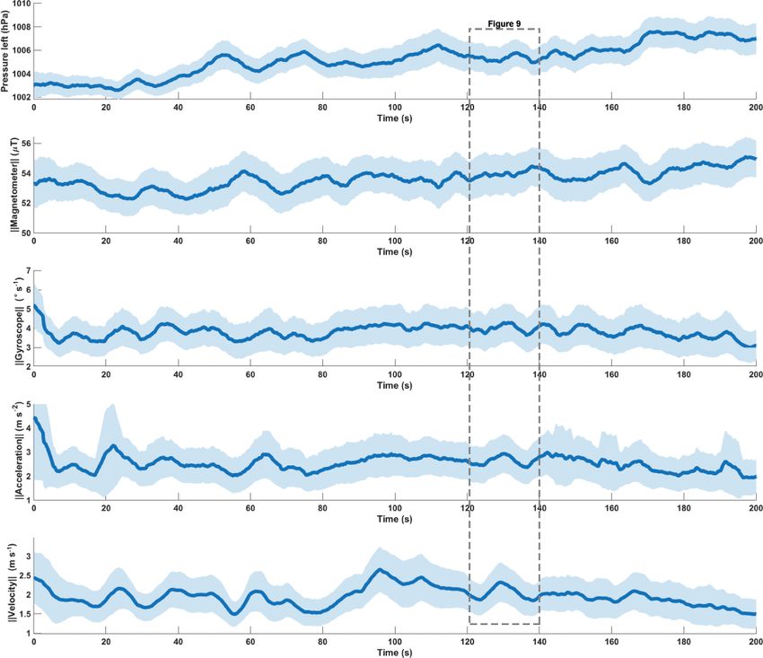
1014                                                                     A. Alexander et al.: Pressure and inertia sensing drifters

Figure 3. (a) Location of the Foxfonna glacier on the Svalbard archipelago. (b) PlanetScope false-color overview of the Foxfonna glacier and
the location of the investigated supraglacial channel acquired on 1 August 2018. (c) Close-up of the studied supraglacial channel. Background
image from PlanetScope acquired on 1 August 2018.

equation from Hou et al. (2018):                                         recorded only for parts of the passage (n = 6) leading to very
                                                                         short datasets.
      2
     Z1−  α
               2                                                          The surface transport speed was calculated by integrating
          2    σ                                                         the acceleration measurements over a rolling time window
n=      2
            ·      ,                                            (4)
      ε        µ                                                         for the remaining 40 deployments (n = 40). The window
                                                                         width was initially randomly chosen for the velocity calcula-
where Z1− 2                                                              tion. Once the three components of the velocity vector were
             α is the standard normal deviate (e.g., Z0.975 =
             2
1.96 for the 95 % confidence interval), ε is the defined pre-            calculated, we defined the transport speed as the magnitude
cision, σ is the standard deviation of the population and µ is           of the velocity. The transport speed was then compared to
the population mean. In this study, we set the desired error of          the estimated transport velocity, which was found by divid-
the sample mean to be within ±10 % of the true value (i.e.,              ing the transport distance (450 m) by the total travel time of
ε = 0.10), 95 % of the time (i.e., Z0.975 = 1.96). The values            the drifter. The integration window size was then readjusted
for σ and µ were then obtained from the statistical analysis             individually for every deployment so that it would be within
of the time series data from all deployments.                            a 10 % error threshold from the drifter’s estimated transport
   To find potential features in the time series and to test the         velocity. By doing so, the individual changes in the observed
degree to which data vary over time, moving means were                   transport velocity are accounted for. As the acceleration in-
calculated over the dataset. The moving means for this study             cludes rapid changes in rigid body motion, for instance due
were calculated over a time window of 5 s, as potential sig-             to impact with the channel walls, we found that integration
nal features were most prominent at this window length, and              produced large outliers, which are not representative of the
plotted together with the 95 % confidence interval (CI). This            water flow itself. Therefore the estimated instantaneous ve-
was done for 40 of the deployments for the first 200 s of the            locities, exceeding 10 m s−1 , were removed.
channel passage. The analysis was limited to the first 200 s,
as not all drifters recorded for the full length of time, so that
a compromise had to be found between maximizing the to-
tal number of deployments and the total duration of deploy-
ment. The other 15 deployments out of the total 55 deploy-
ments were left out as they either recorded no data (n = 9) or

The Cryosphere, 14, 1009–1023, 2020                                                            www.the-cryosphere.net/14/1009/2020/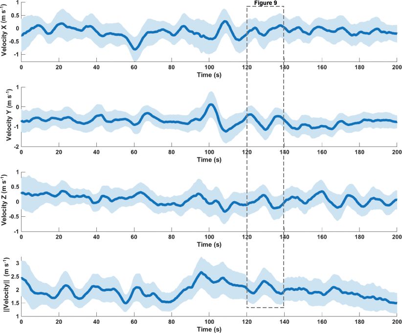
A. Alexander et al.: Pressure and inertia sensing drifters                                                                              1015

Table 1. Recovery and utility rates for supraglacial as well as          Table 2. Estimated multimodal sample sizes for ±10 % precision
englacial–subglacial deployments. The results from the supraglacial      and a 95 % CI based on measured mean values and standard devi-
system are from the second experiment with five drifters and a to-       ations from all deployments (n = 40), as well as estimated sample
tal of 55 deployments in the 450 m long supraglacial channel sec-        sizes for supraglacial and subglacial deployments based on the util-
tion. Subglacial–englacial system rates are based on the assumption      ity rate and the measured mean values and standard deviations.
that the drifters can pass through the system, if the dummies pass
through. The estimated total utility rate for subglacial–englacial de-     Sensor              Required sample    Supraglacial   Subglacial
ployments is based on the dummy deployment, as well as the data            mode                   size estimate
usability rate.
                                                                           Pressure left                     2              3             4
                                                                           Pressure right                    2              3             4
                        Supraglacial     Englacial–subglacial              Magnetometer X                1264           1732          2180
                                                                           Magnetometer Y                  531            728           916
        Recovery rate            1.00                     0.80             Magnetometer Z                  296            406           511
        Utility rate             0.73                     0.58             ||Magnetometer||                  3              4             5
                                                                           Accelerometer X             479 603        656 991       826 902
                                                                           Accelerometer Y               7259           9944         12 516
                                                                           Accelerometer Z           1 382 976      1 894 488     2 384 442
3     Results                                                              ||Accelerometer||               670            918         1155
                                                                           Gyroscope X                 115 419        158109        198 999
3.1    Utility rate                                                        Gyroscope Y              14 309 576     19 602 159    2 4671 683
                                                                           Gyroscope Z                 301 182        412 578       519 280
                                                                           ||Gyroscope||                   281            385           485
In the first experiment, five wooden dummies, of the same
size and buoyancy as the drifter, were deployed in a 2.5 km
long supraglacial, partly englacial channel with features of
subglacial channels (step-pool, glide and chute sequences,               magnitude. The latter should however also be corrected by
and debris at the channel bottom), and four out of five                  the value of the local magnetic field strength, and the num-
dummies were recovered after 72 h. The second experiment                 ber of required deployments is therefore likely to be higher.
consisted of 55 multimodal drifter deployments in a 450 m                   Distance and similarity measures were used to test the
supraglacial channel section, returning a total of 40 useful             repeatability of the datasets. All calculated values for ev-
datasets. The other 15 deployments had datasets of insuffi-              ery sensor modality and statistical measure (chi-squared er-
cient duration (below 200 s, compared to an average transit              ror, Kullback–Leibler divergence, mean average error, mean
time of 360 s), as drifters only recorded part of the deploy-            squared error and data range normalized root mean square)
ments there (n = 6) or recorded no data at all (n = 9). The              are close to zero, thus indicating a high repeatability of the
results for recovery and utility rate are presented in Table 1.          drifter deployments (Table S2 in the Supplement). Our cal-
                                                                         culations of the Pearson correlation coefficients confirm that
3.2    Statistical evaluation                                            the two pressure sensors are redundant (Fig. 4). Additionally
                                                                         there is a correlation between the pressure sensors and the
We calculated the ensemble statistics for all successful de-             magnetometer Y readings. The other sensor modalities rep-
ployments, and numerical values can be found in the Supple-              resent independent variables.
ment (Tables S1 and S2). The mean values and the standard
deviations were then used to estimate the required sample                3.3   Moving mean analysis and velocities
size to achieve a precision of the sample mean to be within
±10 % of the time averages (i.e., ε = 0.10) for 95 % of the              After filtering out all short-term sensor fluctuations with a 5 s
time (i.e., Z0.975 = 1.96). The obtained sample size estimates           rolling time window a clear redundancy between the pressure
were afterwards multiplied with the utility rates to estimate            sensors (Fig. 5), as well as a close correlation between mag-
the required number of supraglacial and subglacial–englacial             netometer Y and pressure readings (Fig. 6), becomes visi-
deployments. The mean pressure values were thereby cor-                  ble. As the experiments are conducted at atmospheric pres-
rected with the calculated air pressure of 941.8 hPa based on            sure conditions with only small elevation change over the
elevation (600 m) and air temperature on 7 August 2018. This             passage, almost homogenous pressure signals should be ex-
calculation resulted in unrealistically high required sample             pected. The plot in Fig. 5, however, shows that the pres-
sizes (Table ). These high numbers are however composed                  sure records are displaying distinct variations including sharp
of several components: one part is caused by the sensor ac-              peaks, sudden increases and drops. These variations are su-
curacy and technical problems causing high variations in the             perimposed on a general increase in the pressure, which
measured data, and the second part of the inaccuracy is due              might be caused by the increasing atmospheric pressures as
to spatial and temporal flow variability between deployments             the drifters are flowing downhill, as well as increasing water
but also along the flow path. The lowest required sample size            depths in the channel. The 95 % CI of the averaged pressure
was for the pressure sensors and the magnetic field intensity            signal can be seen to vary over time but generally follows

www.the-cryosphere.net/14/1009/2020/                                                            The Cryosphere, 14, 1009–1023, 2020
1016 A. Alexander et al.: Pressure and inertia sensing drifters
Figure 4. Pearson product-moment correlation coefficients (r) between the different sensor readings for all deployments (n = 40). The
classification is adapted following Cohen (1992).
the same features as the average, with some features having The velocities in the x direction (sideways in the plane
smaller CIs than others. The values of the 95 % CIs are gen- of the drifters’ longitudinal direction; see also Fig. 1) al-
erally very low and on average do not exceed values above ternate between positive and negative values as the drifters
±0.11 % of the mean pressure value of 1005 hPa. travel through a meandering channel (Fig. 8). Velocities in
Plotting the magnitudes of the different sensor modalities the y direction remained mostly negative and vary between
shows that the obtained signals are not homogeneous over fast and slow zones. The negative values in y direction are
time but rather have pronounced signal variations, as also due to the hydrodynamics of the drifters and the balloon,
visible in the pressure signals. The widths of the CIs of all which together with the currents lead the drifter to face up-
sensor modalities decrease after drifter deployment but vary stream. Every drifter had one balloon attached to achieve
slightly throughout the time series. This is due to the drifters neutral buoyancy. We observed that the currents lead to the
passing through different channel geometries and flow fea- balloon flowing slightly ahead and the drifter facing away
tures at individual velocities. The magnitude of the magne- most of the time, thus leading to negative accelerations and
tometer has the second smallest 95 % CI, with a mean CI velocities in the y direction (longitudinal direction of the
of ±2.45 % of its mean value of 54.6 µT. The other sensor drifter; see Fig. 1). In the z direction (downwards facing
modalities have larger CIs with gyroscope readings being the from the drifters’ longitudinal plane; see Fig. 1) the veloc-
next lowest on the list with a mean CI of ±24.8 % of its mean ities remained mainly positive and vary between zones with
value of 3.8◦ s−1 . The accelerometer has the largest CI, and slower and faster flow. The magnitude of the velocity shows
hence the largest variation of recorded values, with a mean several pronounced signal variations in the time series as
CI of ±34.4 % of its mean value of 2.54 m s−1 . well. Generally values around 2 m s−1 are most common.
The mean value of the 40 deployments, used for acceleration
The Cryosphere, 14, 1009–1023, 2020 www.the-cryosphere.net/14/1009/2020/A. Alexander et al.: Pressure and inertia sensing drifters 1017
Figure 5. Mean values and 95 % CI (shaded area) of the left and right pressure over 40 deployments (n = 40) over the first 200 s of the flow
path passage. The data are averaged over a 5 s time window and across 40 deployments.
integration, is 1.94 m s−1 and the mean 95 % CI is ±24.5 % 4 Discussion
(n = 40).
4.1 Drifter performance
3.4 Signal features of a step-pool sequence
An investigation of a glacial stream using sensing drifters
Video footage was taken periodically during the deployment generally demands a significant number of deployments (Ta-
and allowed to isolate the acceleration and pressure record ble ) to allow for a statistical analysis and to account for
during passage of a small step-pool sequence (Fig. 9). A pro- drifter loss and technical problems, which are expressed by
nounced peak, followed by a drop in the signal for the cho- the calculation of the utility rate. Pressure values are the eas-
sen time period, where the drifter passed over the step-pool iest to acquire, as they need the lowest number of deploy-
sequence is visible. The pressure signal trails behind the ac- ments compared to the much higher deployment numbers for
celeration signal. The video footage shows that the drifter the IMU values. However, the acquisition of flow data with
was speeding up towards the edge of the step, when the pres- sensing drifters in glacial channels will require an unrealis-
sure and the acceleration signal increased (Fig. 9a). As the tic amount of time in the field and the deployment of many
drifter flowed over the edge and dropped into the pool un- drifters simultaneously to reduce field time and the potential
derneath, the pressure and acceleration dropped. Once in the for external factors to influence the measurements (e.g., dis-
pool, the drifter was caught in a recirculating current and re- charge variations). Bagshaw et al. (2012) previously showed
mained in the pool for several seconds. This leads to a drop that drifter passage through glacial channels can take several
of the signals, which stagnate at a lower level before increas- days to weeks, which imposes a practical challenge when it
ing again, once the drifter leaves the pool and flows onward comes to acquiring several hundred to several thousand de-
in the supraglacial channel. ployments for statistical analysis. In practice, this means that
the measurements with sensing drifters will only be possi-
ble with lower statistical significance (p
0.05), as field de-
ployments of several thousand drifters are not realistic. The
number of deployments can be reduced by decreasing the ac-
ceptable error, which is introduced by the sensor accuracy
www.the-cryosphere.net/14/1009/2020/ The Cryosphere, 14, 1009–1023, 20201018 A. Alexander et al.: Pressure and inertia sensing drifters Figure 6. Left pressure and magnetometer in y-direction time series. The plot shows the first 200 s of 40 deployments (n = 40), with a moving mean with a time window of 5 s and the 95 % CI (shaded area). and technical problems, as well as through improved field to geometrical features in the flow path such as step-pool se- deployment and recovery methods. Further technological im- quences and recirculation zones. We did however only record provements of the sensor platform could reduce the signal- videos from 13 deployments and did not measure channel ge- to-noise ratio of the drifters and the data usability rate. A ometries during this field experiment. More field studies with problem with the proposed drifter platform was for exam- known geometry and repeated measurements of geometric ple an occasional loss of battery contact in the battery holder features, which can be detected and classified in the signal due to high impacts, leading to corrupted data. This problem time series and the channel geometry, are therefore required has been subsequently solved in an updated drifter system, to verify this hypothesis. Pressure sensors and magnetometer which was field tested in summer 2019. The recovery during Y seem to produce the most clear signal features. The pres- the presented field tests was done by the installation of a net sure sensors have also the smallest 95 % CI of ±0.11 % rela- inside the glacial stream – a method that works well inside tive to the mean and deliver the most repeatable data with the smaller supraglacial streams. It bears however the challenge lowest error. The CIs for all sensors remain more or less con- of high ice (supraglacial streams) and bed loads (glacier out- stant over time; some CIs are however larger than others as lets) clogging the net. This leads to the net damming up the the sensors travel with different velocities through the chan- water and hence allowing the drifter to flow over the net, re- nel and pass certain geometric features at different times, quiring a regular maintenance of the net to prevent drifter which is not accounted for in the plot over time. A part of loss. High discharge and flow velocities pose additional chal- the higher CIs also comes from the individual drifter move- lenges and therefore require the further development of re- ments, such as rotation rate, which are different for every covery methods. deployment, hence leading to a higher CI. It is however still The analysis of the moving means of the signals shows possible to get pronounced signal features of the IMU read- that clear features become recognizable in some of the sig- ings as well, which can then be linked to geometric features nals over the channel passage. The analysis of videos from of the channel and flow morphology, as shown in the sup- the deployments shows that these patterns seem to be related plementary video sequences. The IMU readings hereby give The Cryosphere, 14, 1009–1023, 2020 www.the-cryosphere.net/14/1009/2020/
A. Alexander et al.: Pressure and inertia sensing drifters                                                                            1019

Figure 7. Left pressure overlaid with the magnitudes of the magnetometer, the gyroscope, the accelerometer and the velocities, obtained from
acceleration integration. The line is the moving mean with a 5 s time window, and the shaded area represents the 95 % CI of 40 deployments
(n = 40).

an extra value compared to a platform only equipped with                integration should however be further constrained with field
pressure sensors, as they can provide the necessary extra in-           measurements in future studies to deduce the error intro-
formation, which will allow us to further distinguish between           duced by the integration. Nevertheless, the average 95 % CI
different geometrical and morphological features of the flow            of ±24.5 % relative to the mean value clearly implies that
and the channel respectively.                                           further improvements are in order.
   Multimodal drifters with inertial measurement units                     It can generally be stated that the proposed multimodal
present a potentially valuable tool to obtain three-                    drifter platform provides repeatable data considering the
dimensional accelerations along the flow path of a glacial              supraglacial field experiments at Foxfonna. The utility rate of
channel. The integration of these data allows us to obtain              73 % in supraglacial channels and 58 % of the total deploy-
three-dimensional velocity estimates along the channel and              ments in englacial–subglacial channels provides a first rea-
to obtain transport surface velocities. This allows for an ini-         sonable estimate of how many sensors a practitioner should
tial first-order-of-magnitude estimate of the large-scale (>            consider deploying.
10 cm) velocity distribution inside glacier channels, offering
a large improvement compared to the state of the art, which             4.2    Glaciological implications
relies on point velocities at certain locations through bore-
holes or integrated velocities along the flow path obtained             This study establishes that multimodal sensing drifters
from dye tracing. The velocities obtained from acceleration             equipped with pressure sensors and an inertial measurement
                                                                        unit present a new tool to obtain repeatable measurements

www.the-cryosphere.net/14/1009/2020/                                                           The Cryosphere, 14, 1009–1023, 2020
1020 A. Alexander et al.: Pressure and inertia sensing drifters
Figure 8. Mean values and 95 % CI of the three velocity components and velocity magnitude of 40 deployments (n = 40) over the first 200 s
of the flow path passage. The data are averaged over a 5 s time window.
in supraglacial channels. Further field studies are needed to field strength and rotation rate while flowing along a glacial
interpret sensor time series to identify specific features cor- channel. The field experiments in this study showed that the
responding to channel morphological types and flow condi- platform used is able to obtain repeatable data in a 450 m
tions. The resulting signal features may be used to provide supraglacial stream section. The multimodal drifter measure-
new insights into the dynamics of glacial hydraulics by over- ments appear however to require a significant number of re-
coming the limitations of existing technologies, which are peated deployments to yield repeatable statistics at a 95 %
typically restricted to a point location or yield only informa- CI. This is due to a combination of technical problems and
tion integrated over the flow path. deployment losses as well as natural flow variability. Rapid
We believe that multimodal sensing drifters can also be changes in channel flows will always cause the recorded sig-
of great value for the modeling community by providing nals to have some variations between deployments. We show
input for various models, like subglacial hydrology (e.g., that it is possible to estimate the number of deployments as
Werder et al., 2013) or supraglacial channel development a percentage of a given sensor mode’s time-averaged value.
(e.g., Decaux et al., 2019). However, additional fieldwork us- It was observed that increasing the error threshold to above
ing ground truth velocities from established measurements 10 % of the time average can significantly reduce the num-
(e.g., tracer studies) as compared to drifter estimates is nec- ber of necessary deployments. The total pressure measure-
essary. Once this is done, other important studies linking sub- ment was found to be the most feasible for repeatable flow
glacial hydrology measurements to glacier dynamics can be path measurements in supraglacial channels, as they consis-
envisaged. tently had the lowest error thresholds and high repeatabil-
ity. After integration and low-pass filtering, the linear accel-
eration allowed for an estimation of flow velocities. An in-
5 Conclusions teresting finding was that the drifter data do not have ran-
dom distributions but rather distinctly non-Gaussian proba-
The multimodal drifter platform tested in this work mea- bility distributions. Comparison of time series events with
sures the total water pressure, linear acceleration, magnetic
The Cryosphere, 14, 1009–1023, 2020 www.the-cryosphere.net/14/1009/2020/A. Alexander et al.: Pressure and inertia sensing drifters 1021
reliable and affordable device for glacial hydrological stud-
ies.
Data availability. All raw data are available under
https://doi.org/10.5281/zenodo.3660488 (Alexander et al.,
2020).
Video supplement. Sample videos of the drifter deployments in
supraglacial channels can be found online as video supplements
(https://doi.org/10.5446/45582, Alexander, 2020).
Supplement. The supplement related to this article is available on-
line at: https://doi.org/10.5194/tc-14-1009-2020-supplement.
Author contributions. AA, MK and JAT designed and planned the
study. AA and MK conducted the fieldwork with support of AJH.
AA analyzed the data and wrote the paper. All authors contributed
to the interpretation of the results and the paper.
Competing interests. The authors declare that they have no conflict
of interest.
Acknowledgements. The transport of Andreas Alexander to and
from Longyearbyen was provided by Oceanwide Expeditions. The
University Centre of Svalbard provided logistical support, and the
Figure 9. Example data of a drifter going over a step-pool sequence. TalTECH IT doctoral school provided support for a research stay
The plot shows the left pressure record as well as the magnitude of of Andreas Alexander in Tallinn for data analyses. This study is a
the acceleration from a single drifter, while passing over a step-pool contribution to the Svalbard Integrated Arctic Earth Observing Sys-
sequence. The data are averaged over a 2.5 s time window. Three tem (SIOS). The reviews of Liz Bagshaw and Samuel Doyle helped
zones are marked on the plot, which represent different parts of the to improve the quality of the paper. We would also like to thank
passage. (a) The acceleration and the total pressure increase as the Samuel Doyle for his second review as well as Jan De Rydt for his
drifter travels towards the edge of the step. (b) The acceleration and editorial work.
the total pressure drop as the drifter flows over the edge. (c) Nearly
constant acceleration and pressure values while the drifter is caught
in an eddy inside the pool. Financial support. This research has been supported by the Euro-
pean Research Council (grant no. ICEMASS), the Research Council
of Norway (grant no. 223254 – NTNU AMOS), the Estonian Re-
search Competency Council (grant no. IUT-339), the Estonian Re-
search Competency Council (grant no. PUT-1690 Bioinspired Flow
video footage of the drifters indicates that rapid variations
Sensing) and the Horizon 2020 FIThydro project.
in the drifter data likely correspond to changes in the chan-
nel morphology (e.g., step-pool sequence) and their corre-
sponding flow characteristics (e.g., turbulent jet or recircu-
Review statement. This paper was edited by Jan De Rydt and re-
lation region). We are optimistic that linking distinct signal viewed by Elizabeth Bagshaw and Samuel Doyle.
variations to channel morphology and flow properties may
provide further insights into unknown channel geometries,
e.g., in subglacial channels. This additional information may
References
provide new, more efficient means to investigate the veloc-
ity distributions within glacial channels. Future field studies Alexander, A.: Sample step-pool sequence from drifter deployment,
including distributed velocity mapping will be carried out to https://doi.org/10.5446/45582, 2020.
further the technological improvements of the proposed plat- Alexander, A., Kruusmaa, M., Tuhtan, J., Hodson, A., Schuler, T.
form, with the long-term objective of providing a new robust, V., and Kääb, A.: Raw data for: Pressure and inertia sensing
www.the-cryosphere.net/14/1009/2020/ The Cryosphere, 14, 1009–1023, 20201022 A. Alexander et al.: Pressure and inertia sensing drifters
drifters for glacial hydrology flow path measurements [Data set], ing of Rivers and Estuaries, in: 2012 Oceans–Yeosu, 1–6,
Zenodo, https://doi.org/10.5281/zenodo.3660488, 2020. https://doi.org/10.1109/OCEANS-Yeosu.2012.6263393, 2012.
Allegretti, M.: Concept for Floating and Submersible Wireless Sen- Diez, A., Matsuoka, K., Jordan, T. A., Kohler, J., Ferraccioli, F.,
sor Network for Water Basin Monitoring, Lect. Notes Com- Corr, H. F., Olesen, A. V., Forsberg, R., and Casal, T. G.: Patchy
put. Sc., 06, 104–108, https://doi.org/10.4236/wsn.2014.66011, Lakes and Topographic Origin for Fast Flow in the Recovery
2014. Glacier System, East Antarctica, J. Geophys. Res.-Earth, 124,
Almeida, T. G., Walker, D. T., and Warnock, A. M.: Estimating 287–304, https://doi.org/10.1029/2018JF004799, 2019.
River Bathymetry from Surface Velocity Observations Using Flowers, G. E.: Hydrology and the Future of the Greenland Ice
Variational Inverse Modeling, J. Atmos. Ocean. Tech., 35, 21– Sheet, Nat. Commun., 9, 2729, https://doi.org/10.1038/s41467-
34, https://doi.org/10.1175/JTECH-D-17-0075.1, 2017. 018-05002-0, 2018.
Arai, S., Sirigrivatanawong, P., and Hashimoto, K.: Control of Fountain, A. G.: Geometry and Flow Conditions of Subglacial
Water Resource Monitoring Sensors with Flow Field Estima- Water at South Cascade Glacier, Washington State, U.S.A.;
tion for Low Energy Consumption, in: 11th IEEE Interna- an Analysis of Tracer Injections, J. Glaciol., 39, 143–156,
tional Conference on Control Automation (ICCA), 1037–1044, https://doi.org/10.3189/S0022143000015793, 1993.
https://doi.org/10.1109/ICCA.2014.6871063, 2014. Germain, S. L. S. and Moorman, B. J.: The Development of
Bagshaw, E., Lishman, B., Wadham, J., Bowden, J., Burrow, S., a Pulsating Supraglacial Stream, Ann. Glaciol., 57, 31–38,
Clare, L., and Chandler, D.: Novel Wireless Sensors for in Situ https://doi.org/10.1017/aog.2016.16, 2016.
Measurement of Sub-Ice Hydrologic Systems, Ann. Glaciol., 55, Gleason, C. J., Smith, L. C., Chu, V. W., Legleiter, C. J.,
41–50, https://doi.org/10.3189/2014AoG65A007, 2014. Pitcher, L. H., Overstreet, B. T., Rennermalm, A. K., Forster,
Bagshaw, E. A., Burrow, S., Wadham, J. L., Bowden, J., Lishman, R. R., and Yang, K.: Characterizing Supraglacial Meltwa-
B., Salter, M., Barnes, R., and Nienow, P.: E-Tracers: Devel- ter Channel Hydraulics on the Greenland Ice Sheet from in
opment of a Low Cost Wireless Technique for Exploring Sub- Situ Observations, Earth Surf. Proc. Land., 41, 2111–2122,
Surface Hydrological Systems, Hydrol. Process., 26, 3157–3160, https://doi.org/10.1002/esp.3977, 2016.
https://doi.org/10.1002/hyp.9451, 2012. Gulley, J., Benn, D., Müller, D., and Luckman, A.: A Cut-
Bartholomew, I., Nienow, P., Sole, A., Mair, D., Cowton, T., and and-Closure Origin for Englacial Conduits in Uncrevassed
King, M. A.: Short-Term Variability in Greenland Ice Sheet Mo- Regions of Polythermal Glaciers, J. Glaciol., 55, 66–80,
tion Forced by Time-Varying Meltwater Drainage: Implications https://doi.org/10.3189/002214309788608930, 2009.
for the Relationship between Subglacial Drainage System Be- Hasnain, S. I., Jose, P. G., Ahmad, S., and Negi, D. C.: Character of
havior and Ice Velocity, J. Geophys. Res.-Earth, 117, F03002, the Subglacial Drainage System in the Ablation Area of Dokriani
https://doi.org/10.1029/2011JF002220, 2012. Glacier, India, as Revealed by Dye-Tracer Studies, J. Hydrol.,
Behar, A., Wang, H., Elliot, A., O’Hern, S., Lutz, C., Mar- 248, 216–223, https://doi.org/10.1016/S0022-1694(01)00404-8,
tin, S., Steffen, K., McGrath, D., and Phillips, T.: The 2001.
Moulin Explorer: A Novel Instrument to Study Greenland Ice Hou, H., Deng, Z., Martinez, J., Fu, T., Duncan, J., Johnson, G., Lu,
Sheet Melt-Water Flow, IOP C. Ser. Earth Env., 6, 012020, J., Skalski, J., Townsend, R., and Tan, L.: A Hydropower Bio-
https://doi.org/10.1088/1755-1307/6/1/012020, 2009. logical Evaluation Toolset (HBET) for Characterizing Hydraulic
Boydstun, D., Farich, M., III, J. M., Rubinson, S., Smith, Z., and Conditions and Impacts of Hydro-Structures on Fish, Energies,
Rekleitis, I.: Drifter Sensor Network for Environmental Moni- 11, 990, https://doi.org/10.3390/en11040990, 2018.
toring, in: 2015 12th Conference on Computer and Robot Vision, Isenko, E., Naruse, R., and Mavlyudov, B.: Water Temper-
16–22, https://doi.org/10.1109/CRV.2015.10, 2015. ature in Englacial and Supraglacial Channels: Change
Chandler, D. M., Wadham, J. L., Lis, G. P., Cowton, T., along the Flow and Contribution to Ice Melting on
Sole, A., Bartholomew, I., Telling, J., Nienow, P., Bagshaw, the Channel Wall, Cold Reg. Sci. Technol., 42, 53–62,
E. B., Mair, D., Vinen, S., and Hubbard, A.: Evolution https://doi.org/10.1016/j.coldregions.2004.12.003, 2005.
of the Subglacial Drainage System beneath the Greenland Jaffe, J. S., Franks, P. J. S., Roberts, P. L. D., Mirza, D.,
Ice Sheet Revealed by Tracers, Nat. Geosci., 6, 195–198, Schurgers, C., Kastner, R., and Boch, A.: A Swarm of Au-
https://doi.org/10.1038/ngeo1737, 2013. tonomous Miniature Underwater Robot Drifters for Explor-
Cohen, J.: A Power Primer, Psychol. Bull., 112, 155–159, ing Submesoscale Ocean Dynamics, Nat. Commun., 8, 14189,
https://doi.org/10.1037/0033-2909.112.1.155, 1992. https://doi.org/10.1038/ncomms14189, 2017.
Curran, J. H. and Wohl, E. E.: Large Woody Debris and Flow Re- Jarosch, A. H. and Gudmundsson, M. T.: A numerical model for
sistance in Step-Pool Channels, Cascade Range, Washington, meltwater channel evolution in glaciers, The Cryosphere, 6, 493–
Geomorphology, 51, 141–157, https://doi.org/10.1016/S0169- 503, https://doi.org/10.5194/tc-6-493-2012, 2012.
555X(02)00333-1, 2003. Kriewitz-Byun, C. R., Tuthan, J. A., Gert, T., Albayrak, I., Kam-
Decaux, L., Grabiec, M., Ignatiuk, D., and Jania, J.: Role of merer, S., Vetsch, D. F., Peter, A., Stoltz, U., Gabl, W., and Mar-
discrete water recharge from supraglacial drainage systems in bacher, D.: Research Overview on Multi-Species Downstream
modeling patterns of subglacial conduits in Svalbard glaciers, Migration Measures at the Fithydro Test Case HPP Bannwil,
The Cryosphere, 13, 735–752, https://doi.org/10.5194/tc-13- in: 12th International Symposium on Ecohydraulics (ISE 2018),
735-2019, 2019. 2018.
D’Este, C., Barnes, M., Sharman, C., and McCulloch, J.: A Low- Kullback, S. and Leibler, R. A.: On Information
Cost, Long-Life, Drifting Sensor for Environmental Monitor- and Sufficiency, Ann. Math. Stat., 22, 79–86,
https://doi.org/10.1214/aoms/1177729694, 1951.
The Cryosphere, 14, 1009–1023, 2020 www.the-cryosphere.net/14/1009/2020/You can also read