Quantification of seasonal and diurnal dynamics of subglacial channels using seismic observations on an Alpine glacier
←
→
Page content transcription
If your browser does not render page correctly, please read the page content below
The Cryosphere, 14, 1475–1496, 2020
https://doi.org/10.5194/tc-14-1475-2020
© Author(s) 2020. This work is distributed under
the Creative Commons Attribution 4.0 License.

Quantification of seasonal and diurnal dynamics of subglacial
channels using seismic observations on an Alpine glacier
Ugo Nanni1 , Florent Gimbert1 , Christian Vincent1 , Dominik Gräff2 , Fabian Walter2 , Luc Piard1 , and Luc Moreau3
1 Université
           Grenoble Alpes, CNRS, IRD, IGE, Grenoble, France
2 Laboratoryof Hydraulics, Hydrology and Glaciology (VAW), ETH Zürich, Zurich, Switzerland
3 Edytem, CNRS, Université de Savoie, Chambéry, France

Correspondence: Ugo Nanni (ugo.nanni@univ-grenoble-alpes.fr)

Received: 11 October 2019 – Discussion started: 8 November 2019
Revised: 26 March 2020 – Accepted: 27 March 2020 – Published: 5 May 2020

Abstract. Water flowing below glaciers exerts a major con-         draulic connection between the two systems. The present
trol on glacier basal sliding. However, our knowledge of           findings provide an essential basis for testing the physics rep-
the physics of subglacial hydrology and its link with slid-        resented in subglacial hydrology and glacier sliding models.
ing is limited because of lacking observations. Here we
use a 2-year-long dataset made of on-ice-measured seismic
and in situ-measured glacier basal sliding speed on Glacier
d’Argentière (French Alps) to investigate the physics of sub-      1   Introduction
glacial channels and its potential link with glacier basal slid-
ing. Using dedicated theory and concomitant measurements           Subglacial water flow exerts a major control on glacier and
of water discharge, we quantify temporal changes in chan-          ice sheet dynamics and their response to variations in water
nels’ hydraulic radius and hydraulic pressure gradient. At         supply (e.g. Iken and Truffe, 1997; Zwally et al., 2002; Sun-
seasonal timescales we find that hydraulic radius and hy-          dal et al., 2011; Bartholomaus et al., 2011; Chandler et al.,
draulic pressure gradient respectively exhibit a 2- and 6-fold     2013; Hewitt, 2013; Brondex et al., 2017; Joughin et al.,
increase from spring to summer, followed by comparable de-         2018). Water flowing at the base of glaciers modulates glacier
crease towards autumn. At low discharge during the early           basal sliding by lubricating the ice–bed interface. The higher
and late melt season channels respond to changes in dis-           the water pressure, the weaker the basal friction, resulting in
charge mainly through changes in hydraulic radius, a regime        faster glacier sliding (Iken and Bindschadler, 1986; Schoof,
that is consistent with predictions of channels’ behaviour at      2005; Gagliardini et al., 2007). Water pressure depends not
equilibrium. In contrast, at high discharge and high short-        only on the total water input but also on the way the water is
term water-supply variability (summertime), channels un-           conveyed through the subglacial drainage system (Lliboutry,
dergo strong changes in hydraulic pressure gradient, a be-         1968), a system that has, yet, yielded limited observations
haviour that is consistent with channels behaving out of equi-     (Flowers, 2015).
librium. This out-of-equilibrium regime is further supported          The subglacial drainage system of hard-bedded glaciers is
by observations at the diurnal scale, which prove that chan-       considered to be twofold. First, cavities form on the down-
nels pressurize in the morning and depressurize in the after-      stream lee of bedrock bumps and are thought to enhance
noon. During summer we also observe high and sustained             basal sliding through reducing the apparent bed roughness
basal sliding speed, which supports that the widespread in-        (Lliboutry, 1968). These cavities constitute a widespread in-
efficient drainage system (cavities) is likely pressurized con-    efficient drainage system associated with high basal water
comitantly with the channel system. We propose that pres-          pressure, slow water flow (of the order of 10−2 m s−1 ; see,
surized channels help sustain high pressure in cavities (and       e.g. Richards et al., 1996) and limited hydraulic conduc-
therefore high glacier sliding speed) through an efficient hy-     tivity. Second, subglacial channels form into the ice from
                                                                   conduit melt by flowing water heat dissipation and close

Published by Copernicus Publications on behalf of the European Geosciences Union.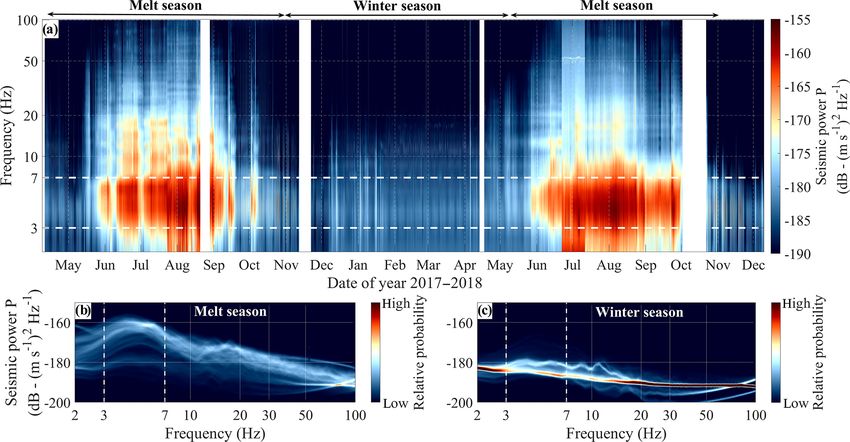
1476                                                 U. Nanni et al.: Subglacial channels’ physics beneath an Alpine glacier

through ice creep (Röthlisberger, 1972; Nye, 1976). These         cavity system, causing an average basal water pressure rise
channels constitute a localized efficient drainage system as-     and subsequent basal sliding speed increase (e.g. Nienow
sociated with lower basal water pressure, faster water flow       et al., 2005; Schoof, 2010; Rada and Schoof, 2018). Dur-
and higher hydraulic conductivity compared to within cav-         ing periods with a well-developed channelized system (e.g.
ities. A drainage system for which a steady water input is        in summer), this behaviour has also been observed because
routed through channels tends to slow basal sliding com-          of channelized system drainage capacity being overwhelmed
pared to if water is predominantly routed through cavities        by the water input changes (Bartholomaus et al., 2008; An-
(e.g. Fountain and Walder, 1998; Schoof, 2010). Most of the       drews et al., 2014), causing pressurized channel flow. These
current subglacial drainage models (Schoof, 2010; Hewitt,         studies have been capable to underline the overall differences
2013; Werder et al., 2013; Gagliardini and Werder, 2018) are      between cavity and channel control on subglacial water pres-
based on this twofold representation. These models succeed        sure over different timescales. However, the lack of dedicated
in capturing the two-way channel–cavity coupling but still        channels’ observations independent of those on cavities and
strongly rely on the choice of model parameters (e.g. cavi-       concomitant with glacier sliding speed measurements ren-
ties and channels’ hydraulic conductivity, channels’ opening      ders a more quantitative characterization of the physics of
and closing rates; see de Fleurian et al., 2018). Observational   subglacial hydrology and its link with sliding difficult.
constraints on these parameters (e.g. water pressure, chan-          Here we use on-ice seismology to explore the evolution
nel properties) and on the channel–cavity-sliding link are,       of subglacial channels over two complete melt seasons. Over
however, very limited because of the limited observations of      the last decade an increasing number of studies have shown
the drainage system and concomitant measurements of basal         the high potential of analysing high-frequency (> 1 Hz) am-
sliding speed (Flowers, 2015; de Fleurian et al., 2018).          bient seismic noise to investigate turbulent water flow and
   Direct observations of the drainage system on temperate        sediment transport in terrestrial rivers and streams (e.g.
glaciers have relied on the analysis of water discharge mea-      Burtin et al., 2008, 2011; Tsai et al., 2012; Schmandt et al.,
sured near glacier outlets (Collins, 1979; Hooke et al., 1985;    2013; Gimbert et al., 2014). The recent work of Gimbert
Tranter et al., 1996, 1997; Anderson et al., 2003; Theakstone     et al. (2016) based on observations of Bartholomaus et al.
and Knudsen, 1989; Chandler et al., 2013), of dye-tracing ex-     (2015) suggests that passive seismology may help fill the ob-
periments (Seaberg et al., 1988; Willis et al., 1990; Nienow      servational gap on the physics of subglacial channels. Gim-
et al., 1996, 1998), of recently exposed subglacial environ-      bert et al. (2016) adapted, to subglacial channels, a physical
ments (Vivian and Bocquet, 1973; Walder and Hallet, 1979),        framework that describes how turbulent water flow generates
of local water pressure borehole measurements (Hantz and          seismic waves and that was initially developed for rivers by
Lliboutry, 1983; Copland et al., 1997; Sugiyama et al., 2011;     Gimbert et al. (2014). Contrary to rivers, subglacial channels
Andrews et al., 2014; Hoffman et al., 2016; Rada and Schoof,      have the capability to be full and thus to undergo pressur-
2018; Gräff et al., 2019) or of radar measurements (Church        ized situations. By applying this modified framework to the
et al., 2019). These methods are mostly point scale and of-       Mendenhall Glacier (Alaska) over a 2-month-long summer
ten focus on the cavity system due to the very narrow extent      period, the authors demonstrate that one can use concomitant
of the channel system (Rada and Schoof, 2018). As a con-          seismic noise and water discharge measurements to continu-
sequence, quantitative information on channels’ long-term         ously and separately quantify relative changes in channel hy-
temporal dynamics is limited such that channels’ properties       draulic pressure gradient and channel hydraulic radius. They
(e.g. size, water flow velocity) and dynamics (e.g. opening       inferred that channels mainly evolve through changes in hy-
and closure rate) remain poorly constrained.                      draulic radius over long timescales (multi-weekly), whereas
   Interactions between channels and cavities are often in-       changes in hydraulic pressure gradient are often short-lived
ferred from evaluating glacier-flow-velocity variations in        (sub-daily to weekly). The use of such an approach to inves-
response to meltwater-supply variability. High and sus-           tigate channel physics on relevant glaciological timescales
tained water supply over monthly timescales (e.g. during the      (e.g. diurnal and seasonal) still remains to be conducted, and
peak melt season) has been linked to glacier deceleration         the resulting channels’ properties remain to be compared to
(Bartholomew et al., 2010; Sole et al., 2013; Tedstone et al.,    other independent observations, such as basal sliding speed.
2013, 2015). This behaviour is related to the fact that chan-     This is the objective of our study.
nels’ development increases the drainage system capacity             We conduct a unique and almost uninterrupted 2-year pas-
and is, therefore, expected to reduce the average basal water     sive seismic survey on Glacier d’Argentière (French Alps),
pressure (Fountain and Walder, 1998). On the contrary, dur-       together with continuous measurements of subglacial water
ing a short-term water-supply increase (e.g. at the early melt    discharge, glacier basal sliding speed and local subglacial
season or at diurnal scales), glacier velocity changes have       water pressure. First, we characterize the subglacial channel-
been observed to occur concomitantly with water-supply            flow-induced seismic power signature and use the model of
changes (Parizek and Alley, 2004; Palmer et al., 2011; Sole       Gimbert et al. (2016) to derive time series of hydraulic pres-
et al., 2013; Doyle et al., 2014; Vincent and Moreau, 2016).      sure gradient and hydraulic radius. We then compare these
This behaviour is mostly related to the pressurization of the     channel properties to the other independent measurements

The Cryosphere, 14, 1475–1496, 2020                                                  www.the-cryosphere.net/14/1475/2020/
U. Nanni et al.: Subglacial channels’ physics beneath an Alpine glacier                                                       1477

of glacier sliding speed and basal water pressure. We also          that Pw scales as
compare our seismically derived observations with the theory
                                                                                 H       14/3
for subglacial channels’ physics proposed by Röthlisberger          Pw (f ) ∝ ζ       W u∗ ,                                    (3)
                                                                                 ks
(1972) to assess the implications of these analysis for chan-
nels’ physics. Finally, we investigate the equilibrium state        where u∗ is river wall shear velocity, W is river width, and
of subglacial channels to discuss the channel–cavity inter-         ζ is a function that accounts for turbulence intensity changes
actions and their potential link with basal sliding through-        with changes in the apparent roughness that depend on H ,
out the melt season. Doing so will also allow us to discuss         the flow depth, and ks , the wall roughness size (Fig. 1).
the applicability of such an approach to improve our general           To relate Pw to subglacial channels’ properties, Gimbert
                                                                                                                             √
knowledge on subglacial hydrology mechanisms of moun-               et al. (2016) expressed the shear velocity as u∗ = gRS,
tain glaciers and ice sheets.                                       where g is gravitational acceleration, R the hydraulic radius
                                                                    and S the hydraulic pressure gradient. The hydraulic radius R
                                                                    is defined as the ratio of the cross-sectional area of the chan-
2     Rational                                                      nel flow to its wet perimeter (Fig. 1). This parameter scales
                                                                    with flow depth for open channel flow. The hydraulic pres-
Here we provide a brief background on the theoretical frame-        sure gradient S is a function of both the water pressure rate of
work of Gimbert et al. (2016), which relates seismic noise          change in the flow direction and the bed slope. For free sur-
and water discharge to subglacial channel-flow properties,          face flow, S equals channel slope. In a case of constant chan-
and that of Röthlisberger (1972), which predicts subglacial         nel slope and channel geometry, increasing S means closed
channel hydraulic pressure gradient and hydraulic radius            and pressurizing channel flow.
scaling as a function of water discharge under certain as-             Gimbert et al. (2016) then expressed water discharge Q
sumptions. Refer to Table C1 in Appendix C for a summary            as a function of water flow velocity Vw using the Manning–
                                                                                                2/3 1/2
of all variables, physical quantities and mathematical func-        Strickler relation Vw = R nS0 , where n0 is Manning’s coef-
tions defined in the following sections.                            ficient (Manning et al., 1891; Strickler, 1981). To study Pw
                                                                    for a subglacial channel flow configuration, Gimbert et al.
2.1    Theory of subglacial channel-flow-induced seismic            (2016) considered that the source-to-station distance is con-
       noise                                                        stant such that changes in Pw are not caused by changes
                                                                    in source (channel) position. Gimbert et al. (2016) then as-
Turbulent water flow in a river or a subglacial channel gen-
                                                                    sumed a constant number N of channels and thus neglected
erates frictional forces F acting on the near boundaries (e.g.
                                                                    the dependency of Pw on N . Here we include the dependency
riverbed or conduit wall), which in turn cause seismic waves
                                                                    of Pw on N by considering that all channels have equal hy-
with given amplitude and spectral signature (Gimbert et al.,
                                                                    draulic radius and hydraulic pressure gradient (i.e. are of sim-
2014). By propagating through a medium (e.g. rock, gravel
                                                                    ilar size and position compared to the seismic station) such
or ice), seismic waves cause ground motion at any location
                                                                    that
x away from the source location x0 (Fig. 1). The relationship
between the force time series F (t, x0 ) applied at x0 in a chan-   Pw ∝ NβR 14/3 S 7/3 ,                                       (4)
nel and the ground velocity time series U (t, x) measured at                   8/3 1/2
                                                                    Q ∝ NβR        S     ,                                      (5)
x can be described from Aki and Richards (2002) as
                                                                    where β is a function of conduit shape and fullness that
                        dG (t, x; x0 )                              may be neglected (see supporting materials of Gimbert et al.,
U (t, x) = F (t, x0 ) ⊗                ,                     (1)
                             dt                                     2016, for details). Combining Eqs. (4) and (5) and neglecting
                                                                    changes in β leads to the two following formulations for Pw :
where G(t) is the displacement Green’s function that con-
verts the force applied at x0 into ground displacement at x,        Pw ∝ R −82/9 Q14/3 N −11/3 ,                                (6)
and the notation ⊗ stands for the convolution operator. The         Pw ∝ S 41/24 Q5/4 N −1/4 .                                  (7)
seismic power P of such a signal is defined over a time pe-
riod T as                                                             From Eqs. (6) and (7) two end-member cases can be eval-
                                                                    uated. If changes in discharge occur at constant channel ge-
             U (f, x)2                                              ometry (i.e. constant R and N) from Eq. (6) we have
P (f, x) =             ,                                     (2)
                T
                                                                    Pw ∝ Q14/3 .                                                (8)
where U (f ) = F(U (t)) is the Fourier transform of the
                                                                    In contrast, if changes in discharge occur at constant hy-
ground velocity time series and f is the frequency. We de-
                                                                    draulic pressure gradient and channel number (regardless of
note Pw as the seismic power induced by turbulent water
                                                                    whether the conduit is full or not) from Eq. (7) we have
flow. Based on a description of the force F (f ) as a func-
tion of flow parameters, Gimbert et al. (2014) demonstrated         Pw ∝ Q5/4 .                                                 (9)

www.the-cryosphere.net/14/1475/2020/                                                         The Cryosphere, 14, 1475–1496, 2020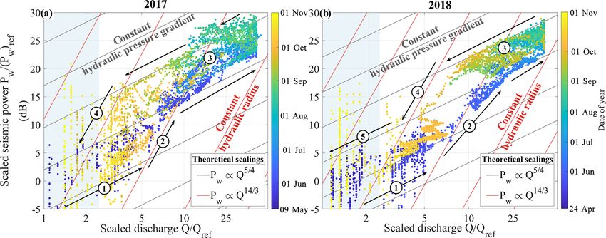
1478                                                    U. Nanni et al.: Subglacial channels’ physics beneath an Alpine glacier

Figure 1. Schematic representation of subglacial channel-flow-induced seismic noise. Representation of an idealized conduit of hydraulic
radius R with a wall shear velocity u∗ (see Eq. 3). Turbulent flow generates frictional forces F , causing seismic waves and resulting in a
ground velocity U that is recorded at a distant seismic station (see Eq. 1).

  Beyond these end-member scenarios, one can use mea-
surements of Pw and Q to invert for relative changes in R
and S using Eqs. (6) and (7) as                                         R ∝ Q9/22 ,                                                   (12)
                                                                                −2/11
                                                                        S∝Q             .                                             (13)
           Pw 24/41 Q −30/41 N 6/41

S = Sref                               ,                      (10)
          Pw,ref      Qref      Nref                                       For a steady-state channel not at equilibrium with Q and

            Pw −9/82 Q 21/41 N −33/82
                                                                   that responds solely through changes in pressure gradient S
R = Rref                                 ,                    (11)      (i.e. R is constant), equations of Röthlisberger (1972) show
           Pw,ref      Qref     Nref
                                                                        that
   where the subset ref stands for a reference state, which
                                                                        S ∝ Q2 .                                                      (14)
has to be defined over the same time period for both Q and
Pw but not necessarily for R and S. Details on the derivation           Further details on the derivation of these equations from
from Eqs. (6) and (7) to Eqs. (10) and (11) can be found in             Röthlisberger (1972) can be found in Supplement Sect. S2.
Gimbert et al. (2016). In the following we consider N to be             Later we compare our inversions of changes in R and S (us-
constant to invert for R and S, and later we prove that our             ing seismic observations) with changes in R and S as pre-
inversions are not significantly biased by potential changes            dicted by the theory of Röthlisberger (1972) for steady-state
in N (Sect. 6.1).                                                       channels at equilibrium or not at equilibrium with water dis-
                                                                        charge.
2.2    R-channel theory

To date, state-of-the art subglacial drainage models use the            3     Field set-up
theories of Röthlisberger (1972) to describe subglacial chan-
nel dynamics (see de Fleurian et al., 2018, for model inter-            3.1    Site and glaciological context
comparisons). Channels described in these theories are as-
sumed to be of semi-circular shape and to form into the ice             Glacier d’Argentière is a temperate glacier located in the
through melt by heat dissipation from the flowing water and             Mont Blanc mountain range (French Alps; see Fig. 2). The
close through ice creep. A channel evolves at steady state              glacier is ca. 10 km long and covers an area of ca. 12.8 km2 .
with water discharge Q if melt and creep rates change in-               It extends from an altitude of ca. 1700 m a.s.l. (metres above
stantaneously with changes in Q. A steady-state channel is              sea level) up to ca. 3600 m a.s.l. in the accumulation zone.
at equilibrium with Q if the melt (opening) rate equals the             Its cumulative mass balance has been continuously decreas-
creep (closure) rate, in which case Röthlisberger (1972) pre-           ing, from −6 m water equivalent (w.e.) in 1975 to −34 m w.e.
dicts                                                                   presently, compared to the beginning of the 20th century
                                                                        (Vincent et al., 2009). This site is ideal for studying sub-
                                                                        glacial channels’ properties, since it presents a typical U-
                                                                        shaped narrow valley (Hantz and Lliboutry, 1983) and hard-
                                                                        bed conditions (Vivian and Bocquet, 1973), two conditions

The Cryosphere, 14, 1475–1496, 2020                                                          www.the-cryosphere.net/14/1475/2020/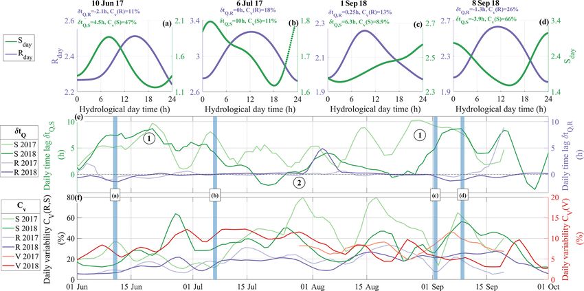
U. Nanni et al.: Subglacial channels’ physics beneath an Alpine glacier                                                     1479

that favour a well-developed R-channel subglacial network          These stations have digitizers of the type Nanometrics
(Röthlisberger, 1972).                                             Taurus, set to 16 Vpp (peak-to-peak voltage) sensitivity and
   In the present study we analyse the data recorded               a 500 Hz sampling rate, and borehole type sensors (model
from spring 2017 to autumn 2018 with seismometers lo-              Lennartz 3D/BH), with an eigenfrequency of 1 Hz. Station
cated between 2350 and 2400 m a.s.l. (Fig. 2). This loca-          ARG.B01 was installed in October 2017 at the centre of
tion corresponds to cross section no. 4 monitored by the           the GDA network, at about 100 m from each GDA stations.
French glacier-monitoring program GLACIOCLIM (https://             The digitizer used for that station is a Geobit SRi32L, set
glacioclim.osug.fr/). There the glacier is up to ca. 280 m thick   to a 10 Vpp sensitivity and a 1000 Hz sampling rate. The
(Hantz and Lliboutry, 1983, updated from a radar campaign          sensor is of the borehole type (model Geobit C100), with an
conducted in 2018). Subglacial water discharge is monitored        eigenfrequency of 0.1 Hz. Station ARG.B02 was installed
600 m downstream of the seismometers at 2173 m a.s.l. near         in April 2018 about 50 m upglacier from station ARG.B01.
the glacier ice fall in subglacial excavated tunnels maintained    The digitizer used for that station is a Geobit SRi32, set to
by the hydroelectric power company Emosson S.A. Sub-               a 0.625 Vpp sensitivity and a 1000 Hz sampling rate. The
glacial water is almost entirely evacuated through one ma-         sensor is of the borehole type (model Geobit S400), with
jor snout, as supported by direct observations of very lim-        an eigenfrequency of 1 Hz. All stations were installed ca.
ited water flowing elsewhere. Thus discharge measured at           5 m deep below the ice surface, except ARG.B02, which
this location is well representative of discharge subglacially     was placed ca. 70 m deep. A few data gaps occurred during
routed under the seismometers’ location. Discharge measure-        our study due to difficulties in ensuring continuous power
ments are conducted from mid-spring to early autumn with           supply and data storage on glaciers.
an accuracy of 0.01 m3 s−1 every 15 min by means of a En-
dress Hauser sensor measuring the water level in a conduit of
known geometry. The minimum measurable value for water
discharge is limited by the measurement accuracy, and the          4     Methodology
maximum value is 10 m3 s−1 due to the capacity of the col-
                                                                   Refer to Table C1 in Appendix C for a summary of all vari-
lector. Because sediments accumulate in the collector, flushes
                                                                   ables, physical quantities and mathematical functions defined
are recorded when the collector is emptied, causing glitches
                                                                   in the following sections.
in the discharge record. We remove these glitches by re-
moving Q values that present d(Q)                          3
                                     dt higher than 0.2 m per      4.1    Calculation of seismic power at a virtual station
15 min. Within the same tunnel network, a subglacial obser-
vatory is used to measure basal sliding speed out of a bicy-       The raw seismic record at each station is first corrected
cle wheel placed in contact with the basal ice (Vivian and         from the sensor and digitizer responses. Then, the frequency-
Bocquet, 1973). Since August 2017 basal sliding speed has          dependent seismic noise power P is computed using the ver-
been measured at a time resolution of 5 s over a 0.07 mm           tical component of ground motion (see Eq. 2). P is cal-
space segmentation. In the close vicinity a pressure sensor, of    culated with Welch’s method over time windows of dura-
the gauge type, is used to measure subglacial water pressure       tion dt with 50 % overlap (Welch, 1967). The longer dt, the
with 10 min time resolution and an accuracy of 400 Pa. The         more likely highly energetic impulsive events are to occur
sensor is installed in a borehole drilled from the excavated       and overwhelm the background noise within that time win-
tunnels up to the glacier bottom (see Vivian and Zumstein,         dow (Bartholomaus et al., 2015). To maximize sensitivity
1973 for details). Air temperature and precipitation measure-      to the continuous, low-amplitude, subglacial channel-flow-
ments are obtained at a 0.5 h time step through an automatic       induced seismic noise and minimize that of short-lived but
weather station maintained by the French glacier-monitoring        high-energy impulsive events, we use a short time window
program GLACIOCLIM and located on the moraine next to              of dt = 2 s to calculate P and average it over time windows
the glacier at 2400 m a.s.l. Precipitation is measured with an     of 15 min in the decimal logarithmic space. We express P
OTT Pluvio weighing rain gauge with a 400 cm2 collecting           in decibel (dB; decimal logarithmic), which allows properly
area. When air temperature is below zero, only precipitation       evaluating its variations over several orders of magnitude.
occurrences are accurate; absolute values are not accurate be-        We reconstruct a 2-year-long time series by merging
cause of snow clogging.                                            records from the five available stations into one unique record
                                                                   at a “virtual” station. To minimize site and instrumental ef-
3.2   Seismic instrumentation                                      fects on seismic power we shift the average power at each
                                                                   station to a reference one taken at ARG.B01. The seismic
We use five seismic stations installed in the lower part of        signal at our virtual station is composed of the GDA seismic
the glacier (Fig. 2). The instruments belong to two seismic        signals between May end December 2017 and of the ARG
networks, denoted as GDA (three stations) and ARG (two             seismic signals between December 2017 and December 2018
stations). Stations GDA.01, GDA.02 and GDA.03 were de-             (see Fig. S1 in the Supplement).
ployed in spring 2017 with ca. 200 m inter-station distances.

www.the-cryosphere.net/14/1475/2020/                                                    The Cryosphere, 14, 1475–1496, 2020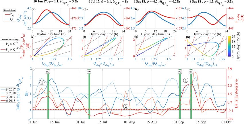
1480 U. Nanni et al.: Subglacial channels’ physics beneath an Alpine glacier
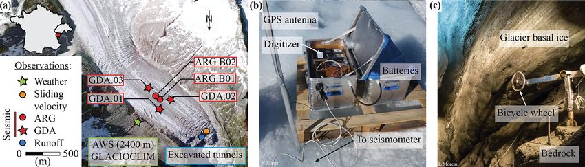
Figure 2. Monitoring set-up of Glacier d’Argentière. (a) Aerial view of Glacier d’Argentière field site (France) and location of the instruments
used in this study. The aerial photography was taken in 2015. The seismic network is composed of the GDA (red circles) and ARG (red stars)
borehole stations and is located according to positions in summer 2018. Station ARG.B02 is installed ca. 70 m deep in the ice, whereas the
four other stations are installed ca. 5 m deep. The GLACIOCLIM (https://glacioclim.osug.fr/, last access: 28 April 2020) automatic weather
station (AWS; green star) provides air temperature and precipitation. Basal sliding speed (orange circle) and water discharge (blue circle) are
measured thanks to direct access to the glacier base from excavated tunnels. Basal water pressure is measured at a similar location to that of
basal sliding speed measurements. (b) Picture of the seismic instrumental set-up used in this study. (c) Picture of the subglacial observatory
with the bicycle wheel used to measure basal sliding speed. Photo credits: (a) IGN France, https://www.geoportail.gouv.fr/ (last access:
28 April 2020), (b) Nathan Maier and (c) Luc Moreau.
4.2 Evaluating bias due to anthropogenic noise ter and use the condition P -PA > 2 dB to define the periods
that evaluate Pw directly from the measurement of P and in-
vestigate the subglacial hydraulic properties.
Later in Sect. 5 we show that when water discharge Q is
low (in the early and late melt season) seismic power from 4.3 Definition of metrics to evaluate sub-diurnal
anthropogenic noise (PA ) is comparable to the subglacial dynamics
channel-flow-induced seismic power (Pw ). Here we evalu-
ate how much PA adding to Pw can bias the evaluation of Since the Pw -versus-Q relationship is not unique and may
scaling predictions of Gimbert et al. (2016). We calculate a vary with time (see Sect. 2), we expect that the diurnal time
synthetic seismic power P as P = PA + Pw and a synthetic series of Pw versus Q may exhibit different patterns through-
Pw from a synthetic Q as Pw = Qn , with n being equal to 45 out the melt season and that these patterns reveal changes in
or 14 the subglacial hydraulic properties. To systematically quan-
3 , as expected from theory (see Eqs. 8 and 9). We quan-
tify the relative contributions of Pw and PA to tify the diurnal variability in Pw , Q, R and S throughout the
hP throughn
the
melt season we define three metrics that we calculate on an
i
parameter Sr , which we define as Sr = log Q P . When
hydrological daily basis (defined as the period between two
Sr tends toward 1, subglacial channel-flow-induced seismic minimum Q values within a 24 h time window). To focus on
power dominates the synthetic seismic power, and when Sr the diurnal variability only, we bandpass-filter our time series
tends towards 0, anthropogenic noise power dominates. within a 6–36 h range (see Appendix Fig. A1 for details). Our
In Fig. 3a we show the temporal evolution of synthetic P first metric quantifies the diurnal variability in a given vari-
with a constant value for PA and with a Pw that responds able X during a given day and corresponds to the coefficient
to a synthetic evolving water supply Q. The value of P of variation Cv , defined as
is normalized by PA , resulting in P = 0 dB in winter. For
Pw ∝ Q14/3 (Fig. 3a; red and orange lines), Pw dominates (Xday )max − (Xday )min
Cv = , (15)
the contribution to P within ca. 10 d of the onset of water Xday
supply. For Pw ∝ Q5/4 (Fig. 3a; black and green lines) P
contains both Pw and PA contributions during a period that is where (Xday )max and (Xday )min are the maximum and mini-
3 times longer than for Pw ∝ Q14/3 . The evolution of Sr with mum value of Xday , respectively, and Xday its average. Our
respect to P -PA (Fig. 3b) is the same for both the constant second metric φ quantifies daily hysteresis between Pw and
hydraulic pressure gradient (red line) and constant hydraulic Q by evaluating the difference between Pw when Q is ris-
radius (grey line) scenarios. For P -PA > 2 dB, Sr is higher ing, e.g. in the morning, and Pw when Q is falling, e.g. in the
than 0.8, meaning that subglacial channel-flow-induced seis- afternoon. Following the approach of Roth et al. (2016), we
mic power contributes by more than 80 % to the synthetic define φ as
seismic power. Later in Sect. 5.2 we measure PA during win-
The Cryosphere, 14, 1475–1496, 2020 www.the-cryosphere.net/14/1475/2020/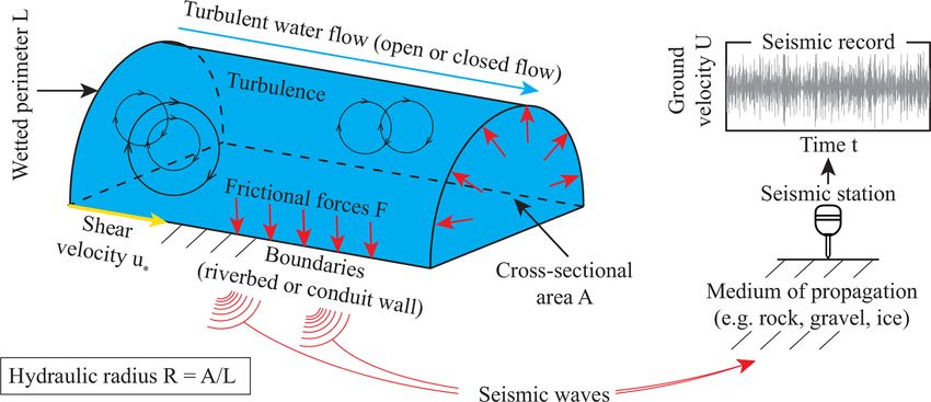
U. Nanni et al.: Subglacial channels’ physics beneath an Alpine glacier                                                                 1481

Figure 3. Synthetic predictions of scaling bias due to anthropogenic noise superimposing on subglacial channel-flow-induced seismic noise.
(a) Synthetic anthropogenic seismic power (green line; PA ), synthetic subglacial channel-flow-induced seismic power Pw = Qn , with Q
being the synthetic water discharge for n = 45 (grey line) and n = 14 3 (orange line) and synthetic seismic power P = PA + Pw for n = 4
                                                                                                                                            5
                     14                                                                                    5                     14
(black line) and n = 3 (red line). (b) Evolution of Sr (see Sect. 4.2) ratio with respect to P -PA for n = 4 (grey line) and n = 3 (red line).
Note that the two curves overlap.

                                                                         are observed within the 2–10 Hz frequency range, in which
                                                                         P is higher by more than 2 orders of magnitude during the
       (Pw,day )rising − (Pw,day )falling                                melt season (mid-May to September) compared to winter.
φ=                                          .                  (16)
                (Pw,day )falling                                         Changes in P are also observed within the 10–20 Hz fre-
                                                                         quency range, with P during the melt season being about an
The larger φ, the more seismic energy is recorded during the
                                                                         order of magnitude larger than in winter. Significant changes
rising discharge period with respect to the falling one. Hys-
                                                                         of smaller amplitude are also observed at higher frequency
teresis can occur either because of an asymmetry between
                                                                         (20–100 Hz). Spectral distributions of P presented in Fig. 4b
(Pw,day )rising and (Pw,day )falling or because of a time lag be-
                                                                         and c show widely spread P values during the melt season
tween Pw and Q. To avoid ambiguity between these two hys-
                                                                         (Fig. 4b; variations over more than 10 dB), as opposed to be-
teresis sources our third metric corresponds to the daily time
                                                                         ing comparatively much narrower in winter (Fig. 4c; varia-
lag δt between the time t ((Pw,day )max ), when Pw is maxi-
                                                                         tions within 1–3 dB). Seismic power within the 3–7 Hz fre-
mum, and the time t ((Qday )max ), when Q is maximum, and
                                                                         quency range shows the highest range of variations from win-
is defined as
                                                                         ter to summer (Figs. 4a and b). Over the 2 years, the overall
δt = t ((Qday )max ) − t ((Pw,day )max ).                      (17)      spectral pattern remains similar, although intra-seasonal vari-
                                                                         ations in P during the 2017 melt season are more pronounced
    We set the condition that for δt to be calculated,                   compared to the 2018 melt season.
t ((Pw,day )max ) has to correspond to both the time when Pw                The observed meteorological and hydrological conditions
is maximum and has a null derivative within a −8–8 h time                at Glacier d’Argentière together with the measured basal
window around t ((Qday )max ). We note that a time delay of              sliding speed and the seismic power P3–7 Hz as averaged
about 0.04 h is expected due to water flowing at ca. 1 m s−1             within the 3–7 Hz frequency range are shown as a function
over the ca. 600 m separating our seismic stations to where              of time (May 2017 to December 2018) in Fig. 5. Water dis-
Q is measured (see Fig. S2 for details). This means that any             charge Q shows a strong seasonal signal, with discharge
values of δt greater than ±0.04 h are not attributable only to           lower than 0.1 m3 s−1 in winter and up to values higher than
water transfer time lags.                                                10 m3 s−1 in summer. These changes are consistent with air
                                                                         temperature values and occur concomitantly with the evolu-
                                                                         tion of P3–7 Hz (Fig. 5b). Further details on the comparison
5     Results                                                            between P3–7 Hz and Q are presented in Sect. 5.2. Over the
                                                                         first months of the melt season (early May to mid-June 2017
5.1    Overview of observations
                                                                         and late April to mid-June 2018), Q increases by about 2 or-
Seismic power P as calculated at our virtual station based               ders of magnitude, from 0.1 to 10 m3 s−1 . At the same time,
on records from our five stations (see Sect. 4) is shown in              the amplitude of the diurnal variations in Q increase up to
Fig. 4a as a function of time (May 2017 to December 2018)                3 m3 s−1 over the summer. The evolution of basal sliding
and frequency (2 to 100 Hz). Large seasonal changes in P                 speed presented in Fig. 5c depicts a rapid acceleration, from

www.the-cryosphere.net/14/1475/2020/                                                             The Cryosphere, 14, 1475–1496, 2020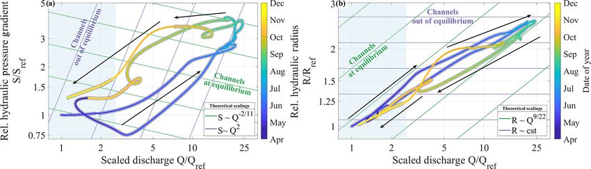
1482 U. Nanni et al.: Subglacial channels’ physics beneath an Alpine glacier
Figure 4. (a) Spectrogram of the observed seismic power P as a function of time (x axis; May 2017 to December 2018) and frequency
(y axis; 1–100 Hz log scale). Colours represent seismic power in decimal logarithmic space (dB; relative to (m s−1 ) 2 Hz−1 ). White bands
correspond to data gaps. (b, c) Spectral distribution of seismic power during the melt seasons (b) and the winter seasons (c). Colours represent
occurrence probability, and colour bars are identical for (b) and (c).
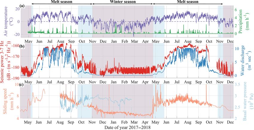
5 mm h−1 in May 2017 and April 2018 to 7 mm h−1 over the within the 2–10 Hz frequency range) nor the concomitant
following month. Sliding speed then stays almost constant temporal evolution of P and Q over the 2 years.
through the summer and slowly decreases down to a min-
imum of 4.5 mm h−1 in February (see also comparable ob- 5.2 Seismic power induced by subglacial channel flow
servations made by Vincent and Moreau, 2016, over the past
decade). Basal water pressure measurements (Fig. 5c) show We consider seismic power P3–7 Hz averaged within the 3–
that at the seasonal timescale the basal water pressure tends 7 Hz frequency range (Fig. 5b; red line) as best representa-
to be higher in winter than in summer by ca. 2.51e+4 Pa. tive of subglacial channel-flow-induced seismic power Pw
In summer 2017 the short-term (diurnal) variability in the because it shows the highest variations with changes in Q
basal water pressure is more pronounced than in winter, as (Figs. 4 and 5). A similar frequency signature of the sub-
also observed for the water discharge (Figs. 5b and A1). glacial channel-flow-induced seismic noise has been ob-
During heavy rainfall (Fig. 5a) and consequent discharge served by Bartholomaus et al. (2015), Preiswerk and Wal-
(Fig. 5b), basal water pressure variations are in phase with ter (2018), and Lindner et al. (2020). This frequency range
sliding speed (Fig. 5c; e.g. on 1 August, 7 August, 18 Au- is also comparable to those observed for water flow in rivers
gust, 30 August, 13 September or 2 October 2017). This evo- (Schmandt et al., 2013; Gimbert et al., 2014). As Q increases
lution of the measured basal water pressure rather depicts a from less than 0.1 m3 s−1 in early May to about 10 m3 s−1 at
local behaviour, whereas changes in the basal sliding speed the end of July, Pw increases by up to 30 dB (i.e. 3 orders of
(Fig. 5c) represent average changes in the average basal wa- magnitude). Differences in relative variations in Pw across
ter pressure conditions over our study area and therefore bet- stations are lower than 0.5 dB, including during periods of
ter represent the global cavity-system pressure conditions. high discharge (Fig. S2). This supports the accuracy and va-
Measurement artefacts are observed for Q, with values lidity of our virtual station reconstruction to study the sub-
having a threshold at 10 m3 s−1 and for P in July 2018, when glacial channel-flow-induced seismic power (Sect. 4). Vari-
unusually high seismic power values are observed over the ations in Pw follow those of Q during the melt season and
whole frequency range, which we associate with the initially over seasonal to weekly timescales (Fig. 5b). Both the high
weak ice-sensor coupling of ARG.B02. Site specificity of the sub-monthly variability in Q and air temperature observed in
GDA network used in 2017 causes higher seismic power in 2017 and the rapid changes in Q occurring in fall 2017 and
the 8–20 Hz frequency band in 2017 than in year 2018. These 2018 are also observed in the temporal evolution of Pw . In
artefacts appear to significantly affect neither P (at least not winter we observe high seismic power bursts from December
to mid-January, occurring when Q is null but concomitantly
with the beginning of heavy snowfall events. These bursts
The Cryosphere, 14, 1475–1496, 2020 www.the-cryosphere.net/14/1475/2020/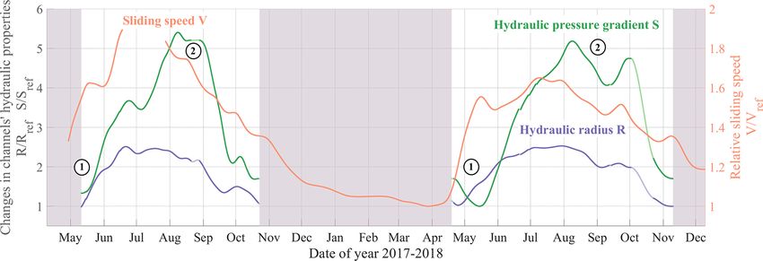
U. Nanni et al.: Subglacial channels’ physics beneath an Alpine glacier 1483
Figure 5. Time series of physical quantities measured from spring 2017 to winter 2018 at Glacier d’Argentière. All data are smoothed over
a 6 h time window. (a) Surface air temperature (purple line) and precipitation (green line) at the GLACIOCLIM AWS (Fig. 2). The dashed
purple line shows T = 0 ◦ C. (b) Averaged seismic power within the 3–7 Hz frequency range at the virtual seismic station (red line; P3–7 Hz ;
see Sect. 5.2 for details) and subglacial water discharge Q (blue line). (c) Basal sliding speed (orange line) and subglacial water pressure
(light blue line) measured at Glacier d’Argentière subglacial observatory (Fig. 2). Note that temporal resolution in the sliding speed is lower
in May–July 2017 and from October 2018 on because of instrumental issues. Red shaded areas represent the winter season; blue shaded
areas represent the periods when diurnal changes in anthropogenic noise are too pronounced to study Pw on a diurnal basis.
are not associated with subglacial channel-flow-induced seis- lows studying the early and late melt season with confidence
mic noise but likely correspond to repeating stick–slip events by reducing the influence of the diurnal variability in PA on
triggered by snow loading similar to those observed previ- Pw while keeping sub-weekly variations in Pw and Q (see
ously by Allstadt and Malone (2014). When Q is lower than Fig. S4 for details).
2 m3 s−1 during winter, early spring and fall, we observe reg-
ular weekly and daily variations in P3–7 Hz that superimpose 5.3 Comparison of observations with predictions from
on the background variations (Fig. 5b). This regular pattern Gimbert et al. (2016)
corresponds to anthropogenic noise, as previously observed
by Preiswerk and Walter (2018) in a similar set-up. 5.3.1 Analysis of seasonal changes
Based on the condition proposed in Sect. 4.2 (P -PA >
Seasonal-scale observations and predictions of the subglacial
2 dB) we use the periods 14 May–1 November 2017 and
channel-flow-induced seismic power Pw versus water dis-
21 April–10 November 2018 to investigate the subglacial hy-
charge Q are shown in Fig. 6. We find that theoretical pre-
draulic properties (white and blue areas in Figs. 5 and 8).
dictions from Gimbert et al. (2016) (red and black lines) are
During these periods we subtract the mean winter diurnal
consistent with our observations (coloured dots), which ex-
pattern of PA (defined between 29 January and 4 April 2018)
hibit a general trend between that predicted at a constant hy-
from P3–7 Hz to obtain Pw (Fig. S3). At the diurnal scale, be-
draulic pressure gradient (Fig. 6; see black lines calculated
cause PA can slightly vary from day to day depending on the
using Eq. 7) and that predicted at a constant hydraulic radius
anthropic activity (e.g. higher anthropic activity during work-
(Fig. 6; red lines calculated using Eq. 6). As Q increases
ing days than holidays), the periods with a very early and
at the very onset of the melt season (in end of April), ob-
very late melt season are still strongly influenced by day-to-
served Pw values follow the trend predicted under constant
day changes in PA . To study diurnal changes in Pw without
hydraulic pressure gradient (Fig. 6 ¬). As Q increases more
being biased by anthropogenic noise we limit our analysis to
rapidly from mid-May to the end of June (Fig. 5b), Pw fol-
the periods 15 May–22 September 2017 and 27 May–28 Oc-
lows a different trend of evolving hydraulic pressure gradient
tober 2018 (white areas in Figs. 5 and 8; based on direct
(Fig. 6 ). The general trend from July to September is then
observation shown in Fig. S3). Later in Sect. 5.4 we filter Pw
dominated by changes in hydraulic radius (Fig. 6 ®). As Q
with a 5 d low-pass filter (i.e. removing variability lower than
decreases during the melt season termination, observed Pw
5 d) when inverting for the hydraulic properties. Doing so al-
values follow the trend of evolving hydraulic pressure gra-
www.the-cryosphere.net/14/1475/2020/ The Cryosphere, 14, 1475–1496, 2020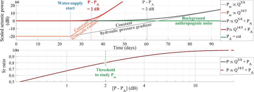
1484 U. Nanni et al.: Subglacial channels’ physics beneath an Alpine glacier
Figure 6. Observed (dots) and predicted (lines) changes in subglacial channel-flow-induced seismic power (PPw) versus changes in water
w ref
discharge QQ during the melt season of 2017 (a) and 2018 (b). Temporal signals are filtered with a 1 h low-pass filter. The colour scale
ref
differs for the 2 years and varies with time from early April to mid-November. Lines show predictions calculated from Eqs. (8) and (9)
for constant hydraulic radii and varying hydraulic pressure gradient (red lines) and for constant hydraulic pressure gradient and varying
hydraulic radii (black lines). Blue shaded areas represent the period when Q is lower than 1 m3 s−1 . Arrows show the direction of time, and
circled numbers refer to periods described in the main text. Reference values (Pw )ref and Qref are taken the first day of the 2017 melt season
(10 May 2018).
dient in a similar manner to during the early melt season focus on these two indicators, as they allow evaluating re-
(Fig. 6 ¯). At the end of the melt season of 2018 (late Oc- spective changes of Pw versus Q.
tober to November) our observations also show a trend of The seasonal evolution of the daily hysteresis amplitude
changing hydraulic radius, although this observation is not φ presents two peaks in late May–early June and in late
as clear in 2017 (Fig. 6 °). A clear counterclockwise sea- August–early September, which are consistently observed in
sonal hysteresis of up to 10 dB power difference is observed both 2017 and 2018 (phases ¬ in Fig. 7i). The seasonal evo-
in Fig. 6 between Pw and Q. This shows that for a similar wa- lution of the diurnal time lag between δt of Pw and Q is sim-
ter discharge, higher subglacial channel-flow-induced seis- ilar to that of φ, with peak values at δt > 2.5 h in late May–
mic power is generated in the late melt season compared to early June and in late August–early September (Fig. 7i). This
the earlier melt season. The 10 m3 s−1 measurement thresh- supports that hysteresis is mainly caused by phase difference
old in Q is well observable for the 2 years but does not bias between Pw and Q rather than by asymmetrical changes Pw
the observed scaling of the changing hydraulic radius ob- when Q rises compared to when Q falls (Sect. 4.3). The vari-
served during summer. ability in δt over the season is much larger than the predicted
0.04 h instrumental time lag (see Sect. 4.3) such that its evo-
lution represents real changes in the relationship between Pw
5.3.2 Analysis of diurnal changes and Q.
In the early and late melt season (phases ¬ in Fig. 7i),
Observations and predictions of the diurnal relationship be- Pw,day peaks, on average, more than 3 h before Qday (e.g.
tween the subglacial channel-flow-induced seismic power Fig. 7e). These long time delay δt values are concomitant
Pw and water discharge Q throughout the melt season are with a pronounced asymmetrical shape in Pw,day , with a
shown in Fig. 7. We quantify the diurnal behaviours over the steeper rising than falling limb (e.g. Fig. 7e). This results
two melt seasons by calculating the hysteresis amplitude φ in large clockwise hysteresis in Pw,day versus Qday as well,
and time lag δt (see Sect. 4.3) and through comparing our shown by the high hysteresis values during these periods
observations with the theoretical predictions calculated for (φ > 1; phases ¬ in Fig. 7i). For example, on 10 June our
4 selected days (Fig. 7a–h). We selected these days based observations follow the trend of evolving hydraulic pressure
on three criteria: they represent typical variations in Pw and gradient in the morning and the one of changing hydraulic
Q over their respective periods (∼ ±5 d around their date), radius in the afternoon and at night. On 8 September our ob-
they show that our observations capture diurnal variations servations follow the trend of changing hydraulic radius in
from unique days without multi-day averaging, and they give the early morning and the one of evolving hydraulic pres-
pedagogical support for the reader to interpret values of the sure gradient in the afternoon. On the contrary to these pe-
hysteresis amplitude φ and time lag δt shown in Fig. 7i. We riods, in summer (phase in Fig. 7i), both φ and δt are
The Cryosphere, 14, 1475–1496, 2020 www.the-cryosphere.net/14/1475/2020/U. Nanni et al.: Subglacial channels’ physics beneath an Alpine glacier 1485
Figure 7. Diurnal observations of the subglacial channel-flow-induced seismic power Pw and water discharge Q and comparison with
predictions from Gimbert et al. (2016). (a–d) Daily evolution of the 6–36 h bandpass-filtered seismic power Pw,day (red line) and water
discharge Qday (blue line) for 4 selected hydrological days. Values of Pw,day and Qday are centred on the average respective absolute value
of the corresponding day. Corresponding values of daily δtQ,Pw and φ are shown at the top of the panels. (e–h) Observed (coloured dots)
and predicted (red and black lines calculated with Eqs. 6 and 7) Pw -versus-Q daily relationships. Note that y axis bounds differ from panel
to panel. Both variables are normalized by their daily minima. (i) Daily time lag δtQ,Pw between Pw,day and Qday peaks (blue lines) and
daily hysteresis φ between Pw,day and Qday (red lines). Shaded lines are data from 2017, and plain ones are data from 2018. Dashed lines
show δtQ,Pw = 0 (blue) and φ = 0 (red). Time series are smoothed over 5 d. Green vertical bars show times of the 4 selected hydrological
days with the corresponding panel number. Circled numbers refer to the two phases described in the main text.
low, with φ ' 0 and 2 h > δt > −2 h. At this time, δt has a and our observations of time series of Q and Pw once fil-
more pronounced seasonal and year-to-year variability than tered with a 5 d low-pass filter (see Fig. S4 and Sect. 5.2 for
φ (Fig. 7i), with values oscillating between −2 and 2 h and details). In the following for the sake of readability we use
minimum values reaching δt < −4 h. In July and August the notation R, S and V to refer to RRref , SSref and the rela-
(e.g. Fig. 7b and c), Pw peaks nearly at the same time as Q tive basal sliding speed VVref . Reference values for these three
with δt < 0.5 h and with an almost symmetrical diurnal evo- variables are taken as their minimum value over the 2 years,
lution (Fig. 7i). For both summer days (6 July and 1 Septem- which occur on 10 May 2017 for R, 14 May 2018 for S and
ber), our observations mainly follow the trend of changing 28 March 2018 for V .
hydraulic radius throughout the whole day, with a non-null
hysteresis that shows that hydraulic pressure gradient may 5.4.1 Analysis of seasonal changes
also change. This two-phase seasonal evolution shows that
diurnal changes in Q in the early and late melt season cause The temporal evolution of R, S and V is presented in Fig. 8.
a pronounced diurnal variability in the hydraulic pressure We recall here that the changes in V can be considered to be
gradient and limited diurnal changes in the hydraulic radius, a good proxy for changes in water pressure in the subglacial
whereas over the summer channels show a more marked re- cavity network (see Sect. 5.1 for details). We find that all
sponse to diurnal changes in Q through changes in hydraulic three variables show a well-marked seasonal evolution, with
radius. low values during the early and late melt season and high
values in summer. However, differences between R, S and V
5.4 Inversions of changes in hydraulic radius and exist over the melt season. For both years, R starts increas-
hydraulic pressure gradient ing from the onset of the early melt season until reaching a
R
maximum within 2 months in late June to early July. R is
We invert for the relative changes of hydraulic radius Rref then 2 times larger on average than in the early melt season.
S
and hydraulic pressure gradient Sref using Eqs. (10) and (11) In contrast, during the first weeks of the melt season 2018,
www.the-cryosphere.net/14/1475/2020/ The Cryosphere, 14, 1475–1496, 20201486 U. Nanni et al.: Subglacial channels’ physics beneath an Alpine glacier
Figure 8. Seasonal evolution of the hydraulic radius and hydraulic pressure gradient as inferred from seismic observations as well as of glacier
basal sliding speed as measured in situ. (a) Relative hydraulic pressure gradient SS (green line), relative hydraulic radius RR (purple line)
ref ref
and relative sliding speed (orange line). Red shaded areas represent the winter season. Temporal signals of R and S are calculated using 5 d
low-pass-filtered time series of Q and Pw and are further smoothed applying a 30 d low-pass filter. Shaded lines correspond with period with
no data and show interpolated values of R and S using a cubic spline interpolation. Reference values for the three variables are taken as their
minimum value of the 2 years (i.e. 10 May 2017 for R, 14 May 2018 for S and 28 March 2018 for V ). Circled numbers refer to the three
phases described in the main text.
S rapidly decreases (Fig. 8 ¬), concomitant with an abrupt scopes as in Sect. 5.3.2 we illustrate, in Fig. 9a–d, the diurnal
increase in V by a factor of 1.5 compared to winter. This evolution of R and S for the same 4 selected days as in Fig. 7.
shows that as the average water pressure rises in cavities and Cv (R) and Cv (S) both present seasonal variation, with
enhances sliding, channels, on the contrary, undergo depres- maximum values being reached mid-summer. The amplitude
surization. During the melt season in 2017 we do not observe of Cv (S) is, however, up to 3 times larger than that of Cv (R),
such behaviour, possibly because of a time series of Pw that since Cv (S) reaches up to 80 % in August, while Cv (R)
starts about 3 weeks later than in 2018. The increase in S only increases up to 30 % (Fig. 9f). In contrast, the seasonal
then occurs with a delay of about 1 month in 2018 and of evolution of δtQ,R and δtQ,S drastically differs (Fig. 9e).
about 1 week in 2017 compared to that in R, and S reaches On the one hand, the temporal evolution of δtQ,R presents
a maximum in August (Fig. 8 ). S is at that time on av- no marked changes throughout the season and generally re-
erage 5 to 6 times larger than in the beginning of the melt mains within a range of ±1 h (Fig. 9e), as highlighted by
season. As S increases, V and R have already passed their the 4 selected days (Fig. 9a to c). This shows that R and Q
summer maximum. Contrary to the conclusions obtained on are consistently in phase on a diurnal basis throughout the
the Mendenhall Glacier (Alaska), where S presents no signif- melt season. On the other hand, the temporal evolution of
icant trend over the 2-month-long investigated period (Gim- δtQ,S presents average values of about 5 h, with two peaks
bert et al., 2016), seasonal changes in water discharge at of δtQ,S > 8 h in June and August (Fig. 9e ¬) and a period
Glacier d’Argentière are inferred to cause changes in both of low values in the range of 0–5 h in mid-summer (Fig. 9e
R and S. From early to mid-September, R and S decrease ). These changes in S are clearly observed in the diurnal
concomitantly and reach their minimum in late October. The snapshots (e.g. Figs. 9a to d) that show a marked increase in
summer-to-winter transition is most pronounced for S, which hydraulic pressure gradient in the morning before the rise in
decreases by about a factor of 4 within less than a month hydraulic radius. Such a difference in diurnal dynamics be-
(September to October), while R decreases more gently. tween R and S shows that channels exhibit high hydraulic
pressure gradients in the early morning time, while their hy-
draulic radius grows slowly to reach its maximum at the same
5.4.2 Analysis of diurnal changes time as the water discharge.
We also compare in Fig. 9f the diurnal dynamics of chan-
nel properties to the diurnal dynamics of the average wa-
Figure 9 describes how channel and cavity properties behave
ter pressure conditions in cavities by comparing Cv (R) and
at the diurnal scale throughout the melt season. We quantify
Cv (S) with Cv (V ). Over the melt season, Cv (V ) exhibits a
the diurnal behaviour throughout the two melt seasons with
pattern that is similar to Cv (R) and Cv (S), with higher val-
the time lag δt between R and Q daily maxima, denoted by
ues observed for the three variables in summer (> 10 %) than
δtQ,R , and between S and Q daily maxima, denoted by δtQ,S .
during the early and late melt season (< 10 %). This shows
We also calculate the amplitude of the diurnal variations Cv
that short-term variability in channels’ properties (i.e. R and
for R, S and V (see Sect. 4.3 for definitions). In the same
The Cryosphere, 14, 1475–1496, 2020 www.the-cryosphere.net/14/1475/2020/U. Nanni et al.: Subglacial channels’ physics beneath an Alpine glacier 1487
Figure 9. Diurnal evolution of the hydraulic radius R and hydraulic pressure gradient S and comparison to glacier dynamics. (a–d) Daily
time series of R (purple line) and S (green line) for 4 selected hydrological days across the melt season. Time series are bandpass-filtered
within 6–36 h. Values of Rday and Sday are centred on the average respective absolute value of the corresponding day. Corresponding daily
values of δtQ,R , δtQ,S , Cv (R) and Cv (S) are shown at the top of the panels. Note that y axis bounds differ from panel to panel. (e) Daily time
lags δtQ,R between Rday and Qday peaks (purple lines) and δtQ,S between Sday and Qday peaks (green lines). (f) Sub-diurnal variability
Cv in R (purple lines), S (green lines) and the basal sliding speed V (red line). Time series are smoothed over 5 d. Blue vertical bars show
location of the 4 selected days with the corresponding panel. Shaded lines are data from 2017, and plain lines are data from 2018. Circled
numbers refer to the two phases described in the main text.
S) correlates well with the short-term variability in average ) changes in S and R with changes in Q significantly depart
water pressure condition in cavities. From late August to from predictions of channels at equilibrium and approach one
mid-September 2017, we observe that Cv (S) reaches up to of the channels evolving out of equilibrium through changes
60 % over less than a week, followed ca. 1 week later by a in S solely. The transition between the two regimes herein
rapid rise in Cv (V ) (Fig. 9f). observed is quite abrupt for S, which switches from being a
decreasing to being an increasing function of Q. For R, the
5.5 Comparison of inversions with predictions from transition is marked by a weaker dependency on Q, as the
Röthlisberger (1972) latter is high. During the period when Q/Qref > 5, the best
data fit of R with Q gives R ∝ Q0.27 ∝ Q6/22 , and for the
Our seismically derived S and R values are shown in Fig. 10 periods when Q/Qref < 4, it gives R ∝ Q0.36 ∝ Q8/22 . The
as a function of relative changes in water discharge Q, along latter scaling is similar to the predicted scaling of R ∝ Q9/22
with scaling predictions calculated using the theory of Röth- calculated using the theory of Röthlisberger (1972) assuming
lisberger (1972), assuming channels at equilibrium (melt rate channels at equilibrium.
equals creep rate) with S ∝ Q−2/11 and R ∝ Q9/22 (Eqs. 14
and 12; green lines in Fig. 10) and channels out of equilib-
rium that respond to changes in Q only through changes in 6 Discussion
S with S ∝ Q2 and R being constant (Eq. 13; purple lines in
Fig. 10). We find that R and S generally exhibit variations 6.1 Evaluating potential bias from changes in the
with Q that lie between those expected for channels at equi- number and position(s) of channel(s)
librium and those expected for channels evolving at constant
hydraulic radius. At low discharge ( QQref < 4, Q < 1 m3 s−1 ) As stated in Sect. 2, the subglacial channel-flow-induced
during the early and late melt season (Fig. 10 ¬) our derived seismic power Pw depends on the number of subglacial chan-
changes in S and R with Q approach the theoretical predic- nels N (Eqs. 10 and 11) and on the source-to-station dis-
tion for channels behaving at equilibrium. At high discharge tance, which we both considered to be constant in our anal-
( QQref > 4, Q > 1 m3 s−1 ; mid-May to early October; Fig. 10 ysis. Here we discuss how much potential changes in N and
www.the-cryosphere.net/14/1475/2020/ The Cryosphere, 14, 1475–1496, 2020You can also read