Environmental interactions during the extreme rain event associated with ex-tropical cyclone Oswald (2013)
←
→
Page content transcription
If your browser does not render page correctly, please read the page content below

CSIRO PUBLISHING

Journal of Southern Hemisphere Earth Systems Science, 2019, 69, 216–238
https://doi.org/10.1071/ES19016

     Environmental interactions during the extreme rain event
     associated with ex-tropical cyclone Oswald (2013)

     Marie-Dominique Leroux A,G, Mai C. Nguyen-Hankinson B, Noel E. Davidson C,
     Jeffrey Callaghan D, Kevin Tory E, Alan Wain F and Xinmei Huang F
     A
       Laboratoire de l’Atmosphère et des Cyclones (Unité Mixte 8105 CNRS/Météo-France/Université
       de La Réunion), 50 bvd du chaudron, 97490 Saint-Denis, de la Réunion, France.
     B
       Department of Mathematical Sciences, Monash University, Melbourne, Vic., Australia.
     C
       Centre for Australian Weather and Climate Research, A partnership between the Australian
       Bureau of Meteorology and CSIRO, Melbourne, Vic., Australia.
     D
       Formerly Bureau of Meteorology, Queensland Regional Forecasting Centre, Brisbane, Qld.,
       Australia.
     E
      Science and Innovation Group, Australian Bureau of Meteorology, Melbourne, Vic., Australia.
     F
      Bureau National Operations Centre, Bureau of Meteorology, Melbourne, Vic., Australia.
     G
       Corresponding author. Email: mariedominique.leroux@gmail.com

     Abstract. Tropical cyclone (TC) Oswald made landfall over north-east Australia as a minimal or Category 1 TC on the
     Australian scale on 21 January 2013. As it moved southward, it intensified over land and produced extreme rainfall for
     nearly 7 days. Tornadoes were reported and confirmed. Tragically, seven people died and insurance estimates were ,$1
     billion. It is demonstrated that the event was associated with an interaction between the ex-Oswald circulation and an
     amplifying Rossby wave, which propagated north-eastward from high latitudes. Diagnoses showed that as the wave
     amplified and broke, a potential vorticity (PV) anomaly (PVA) extended to mid-levels, moved equatorward, merged with
     or axisymmetrised the ex-Oswald circulation through mid-levels. Backward trajectories from locations regularly scattered
     within the mid-level circulation illustrated that the storm transitioned from an isolated vortex into a circulation which was
     strongly influenced by its environment for at least 5 days. During this interaction, PV was advected from the environment
     towards the storm through mid-levels. The heavy rain coincided with the commencement and maintenance of this PV
     injection. The PV injection is quantified and shown to be consistent with PV advection by the mean radial flow. In addition,
     eddy angular momentum convergence in the mid- to upper levels coincided with an intensification of the circulation
     through this region. This was first related to outward transport of anticyclonic momentum by the asymmetric outflow at
     upper levels, followed by inward transport of cyclonic momentum by the asymmetric inflow. It is shown that the
     environmental interaction had an impact on vortex structure changes, rainfall and tornado development. We propose that
     the environmental processes influenced the ascent within the storm (1) via differential vorticity advection and baroclinic
     forcing, as the mid- to upper level PVA approached the circulation and (2) by low- to mid-level warm air advection.

     Received 26 April 2019, accepted 23 October 2019, published online 11 June 2020

1 Introduction                                                        not happen and in fact the storm strengthened after it made
At landfall, tropical cyclones (TCs) pose significant forecast        landfall and as it moved southwards. Other studies in the
problems because of the potential devastation to life and prop-       literature presented cases of TCs reintensifying over land, espe-
erty from strong winds and heavy rain (e.g. Chen 2012). The task      cially over northern Australia (e.g. Emanuel et al. 2008; Evans
of forecasting the distribution and local intensity of rainfall,      et al. 2011). Smith et al. (2015) presented a vorticity perspective
particularly heavy rain, is very challenging. Although most of        of the genesis of TC Oswald over the Gulf of Carpentaria. They
the numerical forecast guidance for the event described here was      indicated that the storm developed on a monsoon shear line and
of good quality, it is still very important to analyse the event to   that intensification continued as the low performed a loop over
see if we can understand the physical mechanisms that produced        land from 18 to 20 January. They showed that moisture levels
such a high-impact rain event.                                        were high enough in the monsoon circulation to enable intensifi-
   After TCs make landfall, they normally weaken and rainfall         cation over land following periodic bursts of convection near the
correspondingly decreases. For the case analysed here, this did       circulation centre that concentrated absolute vorticity.

Journal compilation Ó BoM 2019 Open Access CC BY-NC-ND                                                   www.publish.csiro.au/journals/es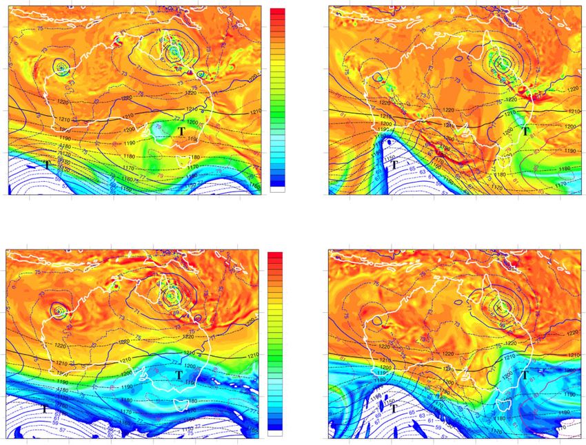
Environmental interactions                                                   Journal of Southern Hemisphere Earth Systems Science       217

    When baroclinic potential energy is available from a west-          investigates the main pathway to Dora’s intensification under an
erly trough, the remnant circulation of a landfalling TC can            upper level trough forcing: ‘The wave activity of a trough can be
revive and even produce enhanced rainfall (Dong et al. 2010;            viewed as large-scale eddy transport of angular momentum, heat
Bosart and Lackmann 1995). However, the precise nature of the           (Molinari and Vollaro 1989, 1990), and potential vorticity
‘interaction’ does not seem to be well understood, and so one           (Molinari et al. 1995, 1998) that may vary in connection with
aim of the current study is to describe it more precisely. There        the storm PV structure evolution. Its impact on the mean
are many studies on the ‘interaction’ between TCs and mid-              tangential flow acceleration can be assessed with Eliassen–Palm
latitude baroclinic environments. Interestingly, they tend to           (E–P) fluxes (Hartmann et al. 1984) computed in a storm-
focus on either the extratropical transition (ET, Evans et al.          following cylindrical and isentropic framework for an adiabatic
2017) of TCs (e.g. Klein et al. 2000; Harr and Elsberry 2000;           frictionless f plane.’ The relative eddy angular momentum flux
Jones et al. 2003; Ritchie and Elsberry 2003, 2007; Anwender            convergence (REAMFC; Molinari and Vollaro 1989) is a
et al. 2008; Keller et al. 2019; Pohorsky et al. 2019) or the           simpler parameter that can be used to quantify the spin-up of a
antecedent rainfall well ahead of TCs (Cote 2007; Stohl et al.          storm’s tangential circulation on a given pressure level due to
2008; Srock and Bosart 2009; Galarneau et al. 2010; Lee and             asymmetric eddies (from Rossby wave activity, for example).
Choi 2010; Bosart et al. 2012; Baek et al. 2013; Moore et al.           Azimuthal eddy flux of angular momentum shows import or
2013). Oswald was not a well-defined ET event, since the                inward flux of cyclonic momentum in the upper troposphere
circulation had made landfall and had weakened below TC                 within rapid intensification cases – the primary features that
intensity before any interaction took place. But it did have many       produce such fluxes are outflow jets and approaching
characteristics of TCs undergoing ET. We show that it was               troughs. The REAMFC is usually computed at 200 hPa over a
clearly an extratropical interaction, and so it bears similarities      300–600-km radial range around the TC centre. An interaction
with ET events. Rainfall mostly occurred following landfall and         is generally said to occur when the REAMFC exceeds
in association with the circulation itself, so it was not an            10 m s1 day1 for at least two consecutive 12-h time periods
antecedent rain event.                                                  (DeMaria et al. 1993; Hanley et al. 2001). This parameter acts as
    Leroux et al. (2016) give a comprehensive review of how             a measure of the outflow layer spin-up of the TC as a trough
upper level troughs or baroclinic forcing can alter the environ-        comes into the aforementioned annulus.
ment of TCs and have different impacts on storm intensity. Their            The geometry of the TC-trough system has been revealed as
numerical simulations of a realistic TC-trough interaction sce-         important in determining how TC intensity will be influenced by
nario suggest that the TC intensity modulation may depend on            a trough (Wei et al. 2016; Leroux et al. 2016; Fischer et al.
the maturity, and hence the vertical depth, of the storm. Vortices      2017). Consistent with observational evidence pointing to the
initially at tropical depression strength intensify much less than      importance of upshear convection on TC intensification after
vortices at tropical storm strength or greater, the latter being able   genesis (e.g. Galarneau et al. 2013), North Atlantic TCs
to benefit from the presence of a trough to reach their maximum         experiencing rapid intensification just after genesis feature
potential intensity (Leroux et al. 2016). Observational analyses        TC-trough configurations that promote stronger quasi-
of TCs at tropical storm strength in the North Atlantic (Fischer        geostrophic ascent to the left of, and upshear of, the TC centre
et al. 2017) and western North Pacific systems (Wei et al. 2016)        and more symmetric convection compared to TC-trough con-
consistently indicate that, overall, upper level troughs promote        figurations where TCs remain at essentially the same intensity
TC intensification. For rapid intensification cases, the potential      (see Fig. 10; Fischer et al. 2017). Overall, these recent studies
vorticity (PV) anomalies associated with the troughs are stron-         suggest that intensification is sensitive to the location of the TC
ger and deeper compared to neutral intensification or slow              relative to the exact position and shape of a nearby trough. In
intensification cases (Fischer et al. 2017). For the TC Dora            particular, Komaromi and Doyle (2018) found that TC-trough
(2007) case, Leroux et al. (2013) showed that PV injection at           interactions are most favourable for intensification when the
mid-levels from a mid-latitude cut-off low or PV coherent               relative distance between the TC and the trough is 0.2–0.3 times
structure could help rapid intensification by increasing convec-        the wavelength of the trough in the zonal direction and 0.8–1.2
tion on the downshear side and sustaining the formation of an           times the amplitude of the trough in the meridional direction.
eyewall replacement cycle (PV budget analysis). They also                   TCs can interact with their environment, such as upper level
noticed that the general 850–200 hPa shear was not indicative           systems, in regions where their inertial stability is the lowest due
of rapid intensification and that it would be more appropriate to       to reduced resistance to radial perturbations. The inertial stabil-
use the 850–500 hPa shear in some cases, which was confirmed            ity of an axisymmetric vortex in gradient balance is defined by
in the recent study of Colomb et al. (2019).                            many sources (e.g. Holland 1987):
    The impact of troughs or mid-latitude baroclinic environ-
                                                                                                                v
ments on TC events that did not intensify has not yet been
                                                                                             I 2 ¼ ðf þ zÞ f þ 2                        ð1Þ
documented in the literature. We want to investigate here if rain                                                r
enhancement, instead of TC intensification, might be an out-
come of such interactions for a TC-making landfall. Environ-            where f is the Coriolis parameter, v the azimuthal mean tangen-
mental interaction will be diagnosed via PV superposition, eddy         tial wind, and r the radius or distance to the centre computed in a
angular momentum convergence and eddy PV fluxes. These                  storm-following cylindrical framework. The maximum inertial
processes and their associated variables are thoroughly                 stability is located in the lower eyewall where the winds and
described in the original study of Leroux et al. (2013) that            cyclonic rotation are maximum. It is lowest at upper levels in the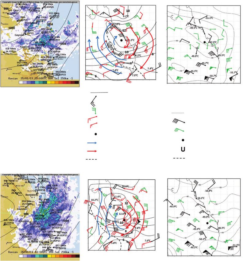
218     Journal of Southern Hemisphere Earth Systems Science                                                           M.-D. Leroux et al.

TC outflow and is also low through mid-levels where outflow is         tornado genesis as ex-TC Oswald moved further down the coast.
generally weak. I2 may evolve in time for TCs impacted by a            Section 9 is the summary and conclusion.
mid-latitude trough, which will be illustrated for ex-TC Oswald.
    Two heavy rain events following the landfalls of TC Fitow
(2013) and TC Bilis (2006) on the China coast were examined by         2 Impacts of rain and wind from ex-tropical cyclone
Bao et al. (2015) and both Deng et al. (2017) and Gao et al.           Oswald
(2009) respectively. In both cases, the torrential rain occurred at    The following description is largely based on Australian Bureau
some 400 km from the storm’s centre. Bao et al. (2015) present         of Meteorology (2013b), Special Climate Statement 44 –
compelling evidence that the Fitow event was influenced by a           extreme rainfall and flooding in coastal Queensland and New
rapidly evolving favourable environment. The large-scale flow          South Wales. The Insurance Council of Australia estimated the
changes appeared to provide (1) inflow channels into the rain          cost of the ex-TC Oswald event at $853 million.
area, which influenced the vertical, kinematic structure over the          The track and intensity of Oswald are shown in Fig. 1.
rain area, and hence the ascent field, and (2) regions for active      Locations of place names used in the text are also indicated.
frontogenesis and its associated secondary circulation, with           At landfall, the central pressure of the system was estimated at
enhanced ascent over the rain area. Deng et al. (2017) offer a         990 hPa. The main feature is that the pressure did not rise much
PV perspective of the vortex structure changes of TC Bilis             over land even over south-east Queensland when the centre was
during the heavy rain event. The increased deformation and             well inland. In the several days following landfall, the storm
weakening of vertical vorticity as Bilis approached the monsoon        even slightly intensified over land and maintained a central
trough contributed to the storm evolving from a closed, tight          pressure of ,990 hPa as it travelled slowly southward. Note that
circulation into a loosely distributed circulation. As a result of     Oswald was slowly moving from 2000 UTC 24 January to 1500
the induced pressure and wind anomalies associated with this           UTC 26 January. Most of the eastern coastal and mountain areas
structure change, an increase in gradient wind imbalance in the        of Australia, extending from ,12 to 308S, experienced very
mid-levels redistributed high PV air from the inner core to outer      heavy rainfall during the period from 22 to 29 January (Fig. 2f).
radii. This redistribution of PV explained the rapid decline of the    The heavy rain coincided with the passage of the ex-TC Oswald
inner core circulation and provided a direct lifting mechanism         circulation. Note the relatively large regions with accumulated
for convection within the outer rainband over land.                    rainfall in excess of 200 mm day1 that extend southward of ex-
    In the following sections, we will enlarge upon these issues       TC Oswald for days 23–27 January (Fig. 2a–e). Fig. 2c and d
for the Oswald case, introduce some additional synoptic- and           shows very heavy rain on 25 and 26 January when Oswald was
meso-scale aspects, analyse some backward trajectories from            slowly moving. On 25 January, areas around Rockhampton
Oswald circulation to evaluate the influence of environmental          recorded rainfall exceeding 300 mm for a 24-h period
flow changes and discuss the relevance of these to the produc-         (Fig. 2c). More interestingly, 24-h total rainfall amounts contin-
tion of heavy rain. The interaction will be described in terms of      ued to increase as the storm gained speed after 1800 UTC 26
PV injection from the environment into the storm circulation,          January (Fig. 2e) and further interacted with its environment
and its impact on the storm will be defined using a detailed PV        (Sections 4–8).
and angular momentum analysis. We will also use the turning                Significant rainfall flood totals are indicated in Table 1 and
wind with height thermal advection diagnostic (Tory 2014;              Fig. 3. Rainfall for the areas between Rockhampton and Gympie
Callaghan and Tory 2014) to explain the location and intensity         alone were heavy enough to break the January monthly rainfall
of rainfall. The major objective is to provide quantitative            records. The most extreme daily rainfall for the week occurred
evidence that the large-scale circulation changes influenced           on 27 and 28 January over the Gold Coast Hinterland and New
the efficiency of the rain systems by producing a highly favour-       South Wales border catchment and the edge of the Brisbane
able thermodynamic and kinematic environment. ‘What main-              river catchment where rainfall for a 24-h period was in excess of
tained the circulation for such a long time after it made landfall?’   700 mm (Mt Castle and Springbrook, Table 1). The Queensland
is the critical question to answer here.                               State Emergency Service received 1800 calls for help in 24 h on
    The manuscript is organised as follows: Section 2 describes        28 January, mostly in the south-east areas of the state. Although
the track of ex-TC Oswald as well as the chronology of the heavy       the Lockyer Creek, Bremer River and the Brisbane River
rain event while listing the serious rain and wind impacts.            flooded (Table 1), impacts in Brisbane were not as severe as
Section 3 presents the data used in the study. Section 4 illustrates   the 2011 floods. Torrential rainfall and flooding also occurred in
the Rossby wave breaking event and the resulting evolving              northern New South Wales particularly near Lismore (Table 1)
synoptic-scale flow. Section 5 describes the thermodynamic and         where evacuations occurred, ,2000 in total. The New South
kinematic structure of the ex-TC Oswald circulation and its            Wales State Emergency Service attended to over 2900 calls for
close environment. Section 6 examines the interaction within           assistance, mostly in the North of the state. Eight New South
the PV framework. Section 7 shows results from backward                Wales river systems had flood warnings in place.
trajectory calculations, used to illustrate possible interactions          Tragically, seven people were killed due to the extreme
with the storm’s environment. Section 8 uses angular momen-            weather over the course of the week. Thousands were forced
tum and other considerations to provide interpretation of the          to evacuate and 2000 people were isolated by floodwaters for
interactions between the environment and the ex-Oswald circu-          some days. Key infrastructure was damaged and destroyed,
lation, consistent with the backward trajectories; it shows how        estimated to cost hundreds of millions of dollars. The rail service
the environmental interaction became strongly conducive to             was closed between Cairns and Townsville, the Weipa port shut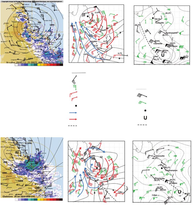
Environmental interactions                                                             Journal of Southern Hemisphere Earth Systems Science             219

                                                                                                                            m

                          14°S                                                                                               1950
                                                                                                                             1875
                                                                                                                             1800
                                                                                                                             1725
                                                                                                                             1650
                          18°S                                                                                               1575
                                                                                                                             1500
                                                                                                                             1425
                                                                                                                             1350
                                                                                                                             1275
                          22°S                                                                                               1200
                                                                                                                             1125
                                                                                                                             1050
                                                                                                                              975
                                                                                                                              900
                          26°S                                                                                                825
                                                                                                                              750
                                                                                                                              675
                                                                                                                              600
                                                                                                                              525
                          30°S                                                                                                450
                                                                                                                              375
                                                                                                                              300
                                                                                                                              225
                                                                                                                              150
                          34°S                                                                                                 75
                                                                                                                                0

                                          140°E           144°E           148°E          152°E          156°E

                          Fig. 1. Best track of Oswald (in blue) showing locations every 6 h and central pressure every 12 h with
                          legend ppp–ddhh, where ppp ¼ central pressure and ddhh ¼ day-time (hour UTC), on top of topography
                          (shaded) and main rivers (in cyan). The 72-h ACCESS-R (IFS) forecast from 0000 UTC 22 January 2013 is
                          shown in red (purple) with locations every 6 h (24 h) and central pressure every 12 h (24 h) with legend
                          ppp–hh, where ppp ¼ central pressure and hh ¼ forecast-time (hours). A black rectangle shows the area
                          used for averages in Fig. 10. Locations are encircled at 0000 UTC synoptic times. ACCESS-R, Australian
                          Community Climate and Earth System Simulator-Regional; IFS, Integrated Forecast System.

down for several days, airlines cancelled many domestic                           south-east under the rainband and warm air advection (WAA)
flights between New South Wales and Queensland, and the                           (see Section 5). On Sunday 27 January, the system impacted
worst ever power outages occurred in Queensland affecting                         Brisbane, the Gold Coast and Sunshine Coast with damaging to
283 000 properties. Overall, Bundaberg was the worst affected                     destructive winds,1 torrential rain, dangerous surf and tidal
city with 2000 homes and 200 businesses inundated with                            inundation for a 24-h period. Winds reached 131 km h1 at Cape
floodwater. The Burnett River was running at ,70 km h1 and                       Byron. The wind impacts can be summarised in Table 2. In
threatened to sweep houses away. Despite a mandatory evacua-                      summary this was a major, high-impact weather event that
tion, 18 helicopters were utilised in a rescue effort evacuating                  needed to be documented and understood.
more than 1000 people trapped by floodwaters in North Bunda-
berg and other most-at-risk areas, which was a record evacuation                  3 Data sources
effort in Australia. On 31 January, in North Bundaberg, ,7000                     The Australian Bureau of Meteorology (BOM) operates a suite
residents were forced out of their homes.                                         of numerical weather prediction (NWP) models, named the
    At many sites, heavy rainfall was accompanied by coastal                      Australian Community Climate and Earth System Simulator
storm surges and big waves, several tornadoes (particularly in                    (ACCESS) (Australian Bureau of Meteorology 2012, 2013a,
the Bundaberg area on Saturday 26 January) as well as strong                      2013b). Objective analyses used in this study are mostly
winds with wind gusts in excess of 100 km h1. When overland                      obtained from ACCESS-G (Australian Community Climate and
on the east coast, there was no maximum wind near the centre                      Earth System Simulator-Global, Australian Bureau of Meteo-
of the storm; the peak winds and tornadoes were well to the                       rology 2012; Puri et al. 2013) at 0.58 resolution. Comparisons

1
  In the Australian context, ‘damaging winds’ are defined as 3-s gusts over open flat land in the range 90–124 km h1. ‘Destructive winds’ are defined as 3-s
gusts over open flat land of 125–164 km h1.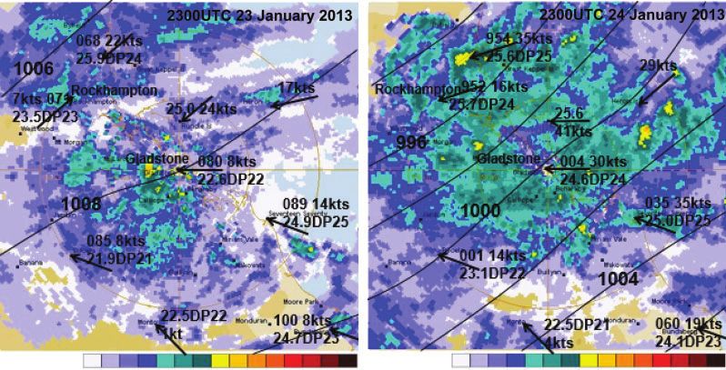
220     Journal of Southern Hemisphere Earth Systems Science                                                                       M.-D. Leroux et al.

                   (a)            23 January          (b)       24 January         (c)      25 January

                                                                                                                    Rainfall (mm)

                                                                                                                            400
                                                                                                                            300
                                                                                                                            200
                                                                                                                            150
                                                                                                                            100
                   (d)          26 January          (e)       27 January           (f )   22–29 January                     50
                                                                                                                            25
                                                                                                                            15
                                                                                                                            10
                                                                                                                            5
                                                                                                                            1
                                                                                                                            0

                   Fig. 2. (a–e) Accumulated daily rainfall totals over Queensland for days 23–27 January and (f) accumulated 7-day
                   rainfall over Australia for the period 22–29 January 2013. These diagrams were obtained from the Bureau of
                   Meteorology site: http://www.bom.gov.au/jsp/awap/rain/index.jsp, accessed 7 May 2020.

                         Table 1. Summary of significant rainfall flood totals associated with Oswald; records are underlined

City                                                 Period                                               Rainfall amount               Previous record

Rockhampton                                          Daily rainfall                                           349 mm                   267.5 mm (1896)
Maryborough                                          Daily rainfall                                          258.8 mm                  250.7 mm (1893)
Yeppoon                                              Daily rainfall                                           289 mm
Mt Castle                                            Daily rainfall (2300 UTC 26–27 January)                  709 mm
Springbrook                                          Daily rainfall (2300 UTC 26–27 January)                  744 mm
Ingham and Tully                                     3-day total rainfall                                    1000 mm

River                                                Comments                                              Flood height               Previous record

Burnett river at Bundaberg                           2.6 m predicted                                           9.3 m
Bremer river                                         15 m predicted                                            13.9 m
Brisbane river                                                                                                   2m
Clarence River at Grafton                            Just below the flood levee wall                           8.09 m
Laidley creek                                                                                              9.26 m on 28           8.85 m (January 2011)
                                                                                                              January

were also made with operational analyses from the global                       0000 UTC 22 January 2013, in particular when compared to that
European Centre for Medium-Range Weather Forecasts                             from the operational IFS model over the same period of interest
(ECMWF) Integrated Forecast System (IFS) at 0.258 resolution                   (Fig. 1, purple colour).
to ensure that the processes discussed here were robust and not                    In ACCESS-R forecasts, the vortex centre is defined as the
the artefact of one model only. Operational regional forecasts                 local extremum in the relative vorticity field at 850 hPa. The use
are from ACCESS-R (Australian Community Climate and Earth                      of the mass-weighted average of the vorticity centres at different
System Simulator-Regional, Puri et al. 2013, Australian Bureau                 levels, local minimum in the mass field or local maximum in the
of Meteorology 2013a), the limited-area configuration of                       wind speed give consistent results. The use of 0.3758-resolution
ACCESS-G, at 0.3758 resolution. ACCESS-R provided a quite                      outputs prevents any mislocation of the TC centre owing to
skilful forecast of the system’s track and intensity from basetime             (1) possible mesovortices with relatively high vorticity in the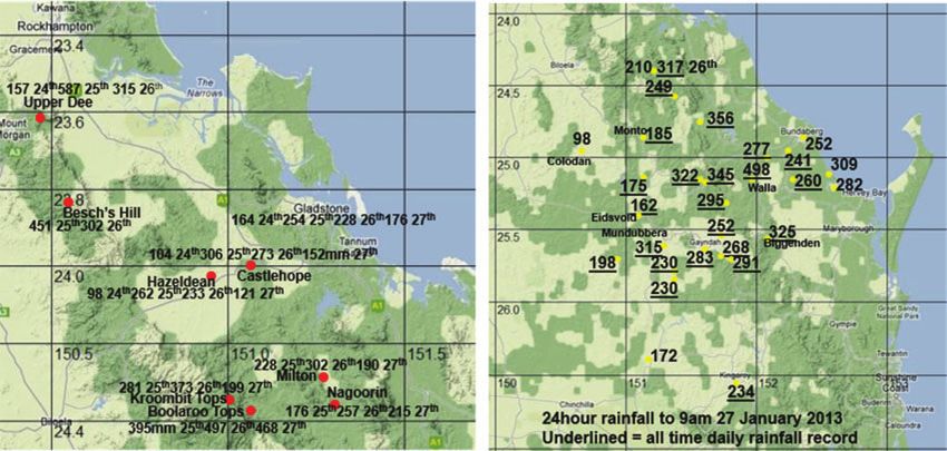
Environmental interactions                                                           Journal of Southern Hemisphere Earth Systems Science            221

             (a)     2300 UTC 22 January– 2300 UTC 26 January                  (b)    2300 UTC 25 January– 2300 UTC 26 January

                                           Large 24 h rainfall (mm)
                                           to 0900 hours 24–27 January 2013

             Fig. 3. (a) Heaviest 24-h rainfall (mm) to 0900 hours 24–27 January 2013 AEST (i.e. UTCþ10 h), that is during the period 2300
             UTC 22–26 January, in the region near Gladstone. (b) Heavy 24-h rainfall to 0900 hours AEST 27 January (2300 UTC 25–26
             January) in and near the Burnett River catchment with all-time record daily rainfall underlined. AEST, Australian Eastern
             Standard Time.

   Table 2. Timeline of significant wind impacts with reports of tornadoes (confirmed) from severe thunderstorms associated with Oswald
AEST, Australian Eastern Standard Time; LT, local time (AEST, i.e. UTCþ10 h); ENE, east-northeast; NE, northeast; SE, southeast; SSW, south-southwest

Time         Town                                                         Reports                Damage and recorded winds
(local)

Saturday 26 January
1300 LT      Bagara (10-km ENE of Bundaberg)                              Tornado or waterspout Two people were critically injured after being trapped in
                                                                           coming ashore from    a car by a fallen tree. Major damage included unroofing
                                                                           over water            of buildings in town, downed power lines, and a car and
                                                                                                 tree which became airborne and dropped into a yard.
                                                                                                 A disaster was declared
1500 LT     Burnett Heads (10-km NE of Bundaberg)                         Tornado               150 homes reported damage
1500 LT     Coonarr (15-km SE of Bundaberg)                               Tornado               Large trees uprooted and strong winds
1608 LT     (,40-km SSW of Bundaberg just east of the Bruce               Tornado
             Highway)
1820 LT     Burnett Heads (10-km NE of Bundaberg)                         Tornado
Sunday 27 January
            Bundaberg, Roma, Peel Island                                                                           90 km h1 3-s gust
            Toowoomba                                                                                              92 km h1 3-s gust
            Redcliffe                                                                                              94 km h1 3-s gust
            Heron Island                                                                                           100 km h1 3-s gust
            Double Island Point                                                                                    122 km h1 3-s gust
Monday 28 January
            Archerfield, Brisbane Airport                                                                          92 km h1 3-s gust
            Gold Coast Seaway                                                                                      94 km h1 3-s gust
            Spitfire Channel                                                                                       96 km h1 3-s gust
            Cape Moreton                                                                                           127 km h1 3-s gust

eyewall region or (2) high vorticity associated with cyclonic                  and deviations from those means are computed. Horizontal
shear away from the storm centre. A cylindrical framework                      bilinear interpolation from a uniform (latitude and longitude)
centred on the TC is chosen to highlight the asymmetric effects                grid to cylindrical coordinates (radius r and azimuth l) is
of the trough on the TC symmetric circulation; azimuthal means                 performed with radial resolution of 40 km and azimuthal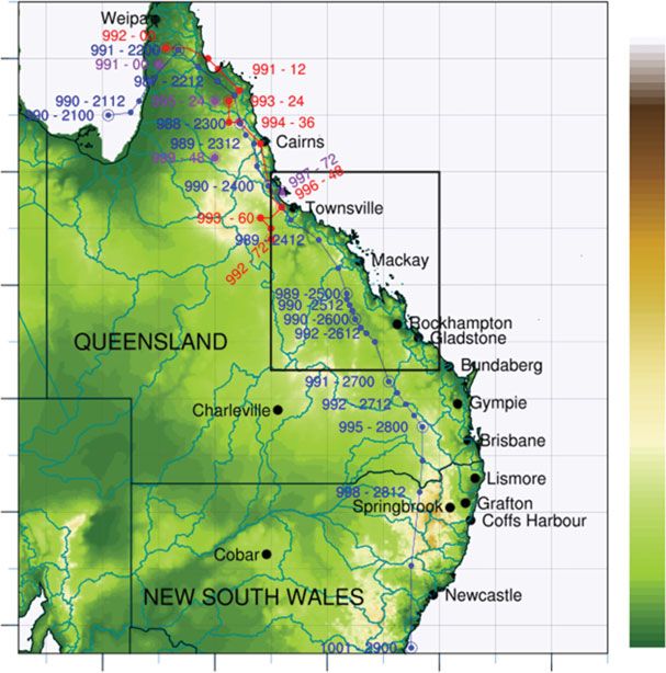
222     Journal of Southern Hemisphere Earth Systems Science                                                             M.-D. Leroux et al.

resolution of 18. Azimuth 08 is east, 908 is north, 1808 is west and    from 23 to 24 January. At 0000 UTC 24 January, the trough is
2708 is south. For diagnostics computed in a storm-relative flow,       located ,1200-km south-southeast of the TC centre (Fig. 6b, d).
the vortex motion is subtracted from the absolute wind at all grid      Examination of the PV coherent structure associated with the
points prior to cylindrical conversion. The wind shear is aver-         trough at both upper (350 K) and mid (330 K) levels suggests that
aged over the 200–800-km annulus range to virtually extract the         it is highly tilted towards the equator. At 330 K, a PV anomaly of
storm vortex (Kaplan and DeMaria 2003).                                 smaller size and amplitude (possibly a cut-off) is advected
   Real-time rainfall analyses of accumulated precipitation are         towards the storm (Fig. 6b), potentially feeding its core with
obtained from the Bureau of Meteorology at http://www.bom.              cyclonic PV from 0000 UTC 24 January. A detailed analysis of
gov.au/jsp/awap/rain/index.jsp, accessed 7 May 2020. The                the PV interaction will be given in Sections 6 and 7.
analysis system is described in Jones et al. (2009). The Bureau              As part of the amplification, an extended, over-the-sea,
of Meteorology archived radar images are from http://www.               easterly trade flow was established to the east of the rain event
theweatherchaser.com/radar-loop/, accessed 7 May 2020.                  (Fig. 5b). This occurred in association with the strengthening in
   The backward trajectories shown here are calculated using            the anticyclone over the south Pacific. We propose that this also
the HYSPLIT Lagrangian trajectory system developed at                   likely provided a continuous supply of moisture for the persis-
NOAA (Draxler and Hess 1998) and implemented at the                     tent heavy rain ahead of the southward moving cyclonic circu-
Australian Bureau of Meteorology (http://www.wmo.int/                   lation. Rainfall was almost certainly modulated by local
pages/prog/www/DPS/WMOTDNO778/rsmc-melbourne-a.                         topography as moist boundary layer air in the extended easterly
htm, accessed 7 May 2020). The trajectories are based upon              flow, associated with the evolving large-scale environment, was
6-hourly data from the ECMWF ERA-Interim reanalysis                     lifted to release conditional instability.
(Dee et al. 2011) at T255 L60 (0.758 latitude–longitude resolu-
tion with 60 vertical levels).                                          5 Thermodynamic and kinematic structures of ex-tropical
                                                                        cyclone Oswald
4 Track and synoptic-scale flow changes – wave activity                 The local kinematic and thermodynamic structure of ex-TC
Apart from its longevity, a peculiarity of the Oswald event is that     Oswald is illustrated in Figs 7 and 8. Figure 7a shows radar-
the cyclone moved parallel to the coastline. The dynamical              based rainfall rates from a composite of Townsville-Gladstone
reasons for this peculiarity are illustrated with a sequence of         radar reflectivities superimposed on the mean sea-level pressure
Global Forecast System (GFS) charts at 850 and 500 hPa from             analysis at 2300 UTC 23 January 2013. The centre of ex-TC
22 to 25 January with actual wind observations for veracity             Oswald was located just to the north-west of Townsville with
(Fig. 4). It clearly shows a north-westward steering flow that          radar indicating moderate patchy rain along the coast to the
dominated the circulation which extended up to 500 hPa from 22          south, where the 700-hPa flow was directed from the warm side
to 27 January (26 and 27 January not shown), resulting in a track       of the 850–500-hPa vertical wind shear to the cold side of it
parallel to the coast. The strong anticyclone over the Tasman           (Fig. 7b), implying WAA or moist isentropic ascent and heavy
Sea (Fig. 5a, b) may have contributed to this north-westward            rainfall (Callaghan 2017a, 2017b; Callaghan and Power 2016;
steering flow and to providing a supply of low-level moisture to        Callaghan and Tory 2014; Tory 2014). A nice illustration is to
the developing system.                                                  look at Brisbane airport at 2300 UTC 26 January when storm
    Synoptic-scale flow changes are illustrated in Fig. 5 with          force winds are turning anticyclonically with height from 850 to
analyses of mean sea-level pressure and 500- and 200-hPa wind           500 hPa (Fig. 8e, see the vertical wind shear in red): 558/55 kts at
prior to and during the event. Apart from the intensification of the    850 hPa, 458/54 kts at 700 hPa and 58/56 kts at 500 hPa. The
ex-TC Oswald circulation (near 198S and 1488E), the dramatic            associated rainfall in the following 24 h was 709 mm at Mt Castle
changes in the large-scale circulation are indicated by (1) the         (247 mm fell in the 9 h following 2300 UTC 26 January) and
strengthening in major anticyclones over the Indian Ocean and           744 mm at Springbrook, which are huge totals for the subtropics.
south Pacific Ocean or Tasman Sea (Fig. 5a, b) and (2) the                  The WAA pattern, indicated by the red streamlines, is
marked amplification of a planetary Rossby wave over higher             associated with the general system-scale cyclonic circulation
latitudes. There is evidence of downstream amplification, indi-         in an environment with nontrivial temperature gradients in the
cated by the succession of developing troughs (Ts) and ridges           low- to mid-troposphere (e.g. Figs. 7b, e and 8b, e). This gradient
(Rs) which propagate towards the north-east (Fig. 5d). There is         appears to be the combination of a general meridional tempera-
also evidence of an ‘interaction’, merger or axisymmetrisation          ture gradient, with a cold-dome super-imposed in the southern
between the propagating wave and ex-Oswald mid-level circula-           edge of the storm (creating a distinct cold-ridge, Fig. 7b, e)
tion. Evidence of this is the large increase in the size of the ex-     associated with the passage of a tropopause undulation above
Oswald mid-level circulation (Fig. 5c, d). This was reflected to        (Fig. 7c, f). The upper level cyclonic PV anomaly casts a shadow
some extent in the size of the low-level TC circulation (Fig. 5a, b).   all the way to the surface, inducing adiabatic ascent for mass
Note that the physical explanation for the downstream amplifica-        continuity, which lifts the isentropes and provides localised
tion from mid-latitudes towards the tropics is Rossby wave              cooling (Hoskins et al. 1985), that is, the 700-hPa cold air centre
breaking that leads to the observed structure in the mid- to upper      evident on Fig. 7b, e. The WAA is a direct result of that cold air
level wind field. The Rossby wave breaking event is clearly             centre. A southward tilt of the storm (Fig. 7e, f) is also consistent
shown on isentropic maps of upper tropospheric PV from IFS              with this temperature structure. The heavy rainfall (Figs 7a, d
operational analyses at 25-km resolution (Fig. 6). The strongest        and 8a, d) is consistent with the diagnosed WAA pattern and
PV values associated with the trough progress towards the tropics       occurs to the south of the storm centre. This region also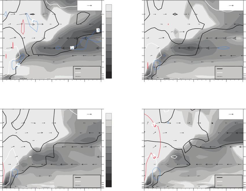
Environmental interactions Journal of Southern Hemisphere Earth Systems Science 223
(a) 850 hPa – 0000 UTC 22 January 2013 (b) 500 hPa – 0000 UTC 22 January 2013
8°S 8°S
55 55
10°S 50 10°S 50
45 45
12°S 40 12°S 40
35 35
14°S 14°S
30 30
25 25
16°S 16°S
20 20
18°S 15 18°S 15
10 10
20°S 5 20°S 5
0 0
22°S 22°S
130°E 132°E 134°E 136°E 138°E 140°E 142°E 144°E 146°E 148°E 150°E 130°E 132°E 134°E 136°E 138°E 140°E 142°E 144°E 146°E 148°E 150°E
80 60
(c) 850 hPa – 0000 UTC 23 January 2013 (d) 500 hPa – 0000 UTC 23 January 2013
8°S
8°S
55 55
10°S
10°S 50
50
12°S 45 45
12°S
40 40
14°S 35
35 14°S
30 30
16°S
16°S 25
25
20 20
18°S
18°S
15 15
20°S 10 10
20°S
5 5
22°S 0
0 22°S
24°S
24°S
136°E 138°E 140°E 142°E 144°E 146°E 148°E 150°E 152°E 154°E 156°E 136°E 138°E 140°E 142°E 144°E 146°E 148°E 150°E 152°E 154°E 156°E
70 50
(e) 850 hPa – 0000 UTC 24 January 2013 (f) 500 hPa – 0000 UTC 24 January 2013
12°S 12°S
55 55
14°S 50 14°S 50
45 45
16°S 16°S
40 40
35 35
18°S 18°S
30 30
20°S 25 20°S 25
20 20
22°S 22°S
15 15
10 10
24°S 24°S
5 5
26°S 0 26°S 0
28°S 28°S
136°E 138°E 140°E 142°E 144°E 146°E 148°E 150°E 152°E 154°E 156°E 136°E 138°E 140°E 142°E 144°E 146°E 148°E 150°E 152°E 154°E 156°E
70 60
(g) 850 hPa – 0000 UTC 25 January 2013 (h) 500 hPa – 0000 UTC 25 January 2013
14°S 14°S
55 55
16°S 50 16°S 50
45 45
18°S 18°S
40 40
20°S 35 20°S 35
30 30
22°S 22°S
25 25
20 20
24°S 24°S
15 15
26°S 10 26°S 10
5 5
28°S 28°S
0 0
30°S 30°S
138°E 140°E 142°E 144°E 146°E 148°E 150°E 152°E 154°E 156°E 158°E 138°E 140°E 142°E 144°E 146°E 148°E 150°E 152°E 154°E 156°E 158°E
80 60
Fig. 4. Global Forecast System wind analyses (knots) at (left frames) 850 hPa and (right frames)
500 hPa for (a, b) 0000 UTC 22 January, (c, d) 0000 UTC 23 January, (e, f) 0000 UTC 24 January
and (g, h) 0000 UTC 25 January 2013. Actual observations of wind, temperature and geopotential
height (m) are plotted where available.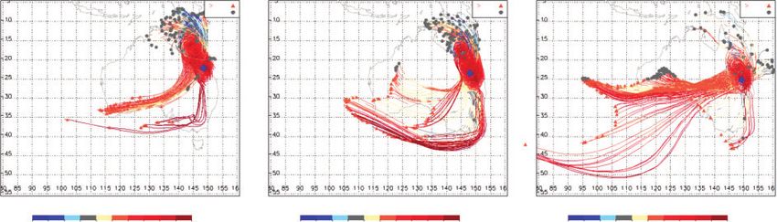
224            Journal of Southern Hemisphere Earth Systems Science                                                                       M.-D. Leroux et al.

      (a)               MSLP – 0000 UTC 20 January 2013                          (b)               MSLP – 0000 UTC 24 January 2013
           90     100   110   120    130   140   150   160    170     180          90        100   110   120   130    140    150    160     170    180
       0                                                                     0    0                                                                        0

      10                                                                    10   10                                                                       10

      20                                                                    20   20                                                                       20

      30                                                                    30   30                                                                       30

      40                                                                    40   40                                                                       40

      50                                                                    50   50                                                                       50

      60                                                                    60   60                                                                       60

           90     100   110   120    130   140   150   160    170     180             90     100   110   120   130    140    150    160      170   180

      (c)           WIND 500 hPa – 0000 UTC 20 January 2013                      (d)           WIND 500 hPa – 0000 UTC 24 January 2013
           90     100   110   120    130   140   150   160    170     180               90   100   110   120    130    140    150    160     170    180
       0                                                                     0    0                                                                        0

      10                                                                    10   10                                                                       10

      20                                                                    20   20                                                                       20

      30                                                                    30   30                                                                       30

      40                                                                    40   40                                                                       40

      50                                                                    50   50                                                                       50

      60                                                                    60   60                                                                       60

           90     100   110   120    130   140   150   160    170     180               90   100   110   120    130    140    150    160     170 180
                                                              0.200E+02                                                                      0.200E+02

      (e)           WIND 200 hPa – 0000 UTC 20 January 2013                      (f )          WIND 200 hPa – 0000 UTC 24 January 2013
          90      100   110   120   130    140   150   160   170    180               90     100   110   120   130    140    150    160      170   180
      0                                                                     0     0                                                                       0

  10                                                                      10     10                                                                      10

  20                                                                      20     20                                                                      20

  30                                                                      30     30                                                                      30

  40                                                                      40     40                                                                      40

  50                                                                      50     50                                                                      50

  60                                                                      60     60                                                                      60

          90      100   110   120   130    140   150   160   170    180               90     100   110   120   130    140    150    160      170   180
                                                              0.400E+02                                                                      0.400E+02

  Fig. 5. Australian Community Climate and Earth System Simulator-Global analyses of (a, b) mean sea-level pressure (MSLP), (c, d) 500-hPa winds
  and (e, f) 200-hPa winds, valid at 0000 UTC 20 January (left panels) and 24 January (right panels) 2013. Contour interval for MSLP is 2 hPa. At 500 hPa,
  contour interval is 10 m s1, with winds greater than 10 m s1 and less than 30 m s1 shaded yellow, and winds greater than 30 m s1 shaded red. At
  200 hPa, contour interval is 20 m s1, with winds greater than 20 m s1 and less than 40 m s1 shaded yellow, and winds greater than 40 m s1 shaded
  red. (d) Troughs and ridges are indicated by T and R symbols respectively.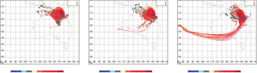
Environmental interactions Journal of Southern Hemisphere Earth Systems Science 225
(a) 330 K – 0000 UTC 23 January 2013 (b) 330 K – 0000 UTC 24 January 2013
PVU
0.8
0.6
0.4
10°S 0.2 10°S
0.0
–0.2
–0.4
–0.6
–0.8
–1.0
20°S –1.2 20°S
–1.4
–1.6
–1.8
–2.0
–2.2
–2.4
30°S –2.6 30°S
–2.8
–3.0
–3.2
–3.4
–3.6
–3.8
40°S –4.0 40°S
–4.5
–5.0
–5.5
–6.0
–6.5
–7.0
50°S 50°S
110°E 120°E 130°E 140°E 150°E 160°E 110°E 120°E 130°E 140°E 150°E 160°E
(c) 350 K – 0000 UTC 23 January 2013 (d) 350 K – 0000 UTC 24 January 2013
PVU
0.8
0.6
0.4
10°S 0.2
10°S
0.0
–0.2
–0.4
–0.6
–0.8
–1.0
20°S –1.2
20°S
–1.4
–1.6
–1.8
–2.0
–2.2
–2.4
30°S –2.6 30°S
–2.8
–3.0
–3.2
–3.4
–3.6
–3.8
40°S –4.0 40°S
–4.5
–5.0
–5.5
–6.0
–6.5
–7.0
50°S 50°S
110°E 120°E 130°E 140°E 150°E 160°E 110°E 120°E 130°E 140°E 150°E 160°E
Fig. 6. Integrated Forecast System operational analyses valid at 0000 UTC 22 January (left panels) and 24 January (right panels) 2013. Plotted are the
Ertel potential vorticity (PV) field on the (a, b) 330-K or (c, d) 350-K isentropic surfaces (shaded; 1 PVU 106 m2 K s1 kg1), the geopotential height Z
(mgp) at 200 hPa (black contours), and the geopotential height Z (mgp) at 925 hPa (blue contours for lows and red contours for highs). Oswald’s best track
centre is indicated by a cross. Troughs are indicated by a T symbol.
experiences topographic lifting of the moist boundary layer et al. 2014 and modelling study by Euler et al. 2019). Note that the
easterlies (Section 4), which would have also favoured rainfall. classical ET structure with a trough to the west was not evident for
Note that the strengthening of the WAA pattern (Fig. 8b, e) from Oswald. Instead there was a merger, as PV from the trough was
26 January coincides with the heaviest rain (Section 2, Figs. 2 axisymmetrised to become part of the TC circulation through
and 3). In the case of ex-TC Oswald, the strength of the WAA mid-levels. It would be interesting to investigate in more depth
along with the high dew points highlighted in Figs 8a, d and 9 what differentiated the Oswald interaction from ET.
can, therefore, explain the extreme rainfall from 24 to 27 To illustrate the vertical structure of the storm, Fig. 10 shows
January (Section 2) that occurred as the storm was interacting forecast time-height sections from the operational regional
with its environment. forecast model ACCESS-R. Sections are computed over a
Another indication of the WAA set-up is the cold air advection rectangular latitude–longitude box (18–258S and 146–1528E)
(CAA) counterpart downstream. A broad band of descent flows that represents the environment preceding the passage of the
northward towards the vicinity of the excyclone circulation. This storm through the box (Fig. 1). Note that at the initial time of
analysis suggests a link with a deep descending current from the the forecast the storm was located near 148S, 1428E, well to the
tropopause undulation up to the circulation of the cyclone as the north-west of the box (Fig. 1). The zonal wind section (Fig. 10a)
undulation passed south of the cyclone, which will be further shows the strengthening in the low-level easterlies and upper
discussed in the PV analysis (Section 6). Note that the deep level westerlies as the storm approaches and begins to feel the
descending current from the tropopause is also a typical indicator effects of the low-level easterlies and upper level westerlies
for TCs undergoing ET (e.g. observational analysis by Quinting associated with the evolving environment. Relative humidity226 Journal of Southern Hemisphere Earth Systems Science M.-D. Leroux et al.
(a) (b) (c)
TMPprs 700 00Z24JAN2013 TMPprs 200 00Z24JAN2013
14°S 14°S
16°S
16°S
18°S
18°S
20°S
20°S
22°S
22°S
24°S
24°S
26°S
26°S
28°S
28°S
30°S
30°S
32°S
32°S
34°S
Rain Rate 138°E 140°E 142°E 144°E 146°E 148°E 150°E 152°E154°E 156°E 158°E 160°E 34°S
138°E 140°E 142°E 144°E 146°E 148°E 150°E 152°E 154°E 156°E 158°E 160°E
Light Moderate Heavy
700 hPa isotherms
700 hPa wind observation
700 hPa reanalysis derived winds
200 hPa isotherms
850–500 hPa vertical wind shears
200 hPa wind observations
850–500 hPa reanalysis shears
200 hPa reanalysis derived winds
Mean sea level centre location
Mean sea level centre location
Cold air advection
Tropopause undulation
Warm air advection
Trough line Trough line
(d ) (e) (f )
TMPprs 700 00Z25JAN2013 TMPprs 200 00Z25JAN2013
14°S 14°S
16°S 16°S
18°S 18°S
20°S 20°S
22°S 22°S
24°S 24°S
26°S 26°S
28°S 28°S
30°S 30°S
32°S 32°S
Rain Rate
Light Moderate Heavy 34°S 34°S
138°E 140°E 142°E 144°E 146°E 148°E 150°E 152°E 154°E 156°E 158°E 160°E 138°E 140°E 142°E 144°E 146°E 148°E 150°E 152°E 154°E 156°E 158°E 160°E
Fig. 7. (a, d) Sea-level isobars and averaged winds overlaid on radar imagery for (a) Townsville at 2300 UTC 23 January and (d) Gladstone at 2300 UTC
24 January. (b, e) At 0000 UTC from 24 to 25 January: 700-hPa winds overlaid on isotherms (solid black contours plotted at 18C-interval) with 850–500-hPa
vertical wind shear in red (smaller barbs representing wind shear computed from reanalysis winds). Green wind barbs are 700-hPa reanalysis winds,
whereas larger black barbs are actual 700-hPa wind observations. Actual temperatures are plotted in black (8C), solid black circle denotes cyclone position,
large blue streamlines denote cold air advection (implying descent) and red streamlines denote warm air advection (implying ascent). (c, f) At 0000 UTC
from 24 to 25 January: 200-hPa winds overlaid on 200-hPa reanalysis isotherms with actual 200-hPa temperatures plotted in black; green wind barbs are
200-hPa reanalysis winds; ‘U’ denotes position of tropopause undulation; the dashed line is a trough line. The reanalysis data are from the US site https://
www.esrl.noaa.gov/psd/data/gridded/data.ncep.reanalysis.html, accessed 7 May 2020.Environmental interactions Journal of Southern Hemisphere Earth Systems Science 227
(a) (b) (c)
TMPprs 700 00Z26JAN2013 TMPprs 200 00Z26JAN2013
14°S 14°S
16°S 16°S
18°S
18°S
20°S
20°S
22°S
22°S
24°S
24°S
26°S
26°S
28°S
28°S
30°S
30°S
32°S
32°S
34°S
Rain Rate 138°E 140°E 142°E 144°E 146°E 148°E 150°E 152°E 154°E 156°E 158°E 160°E
34°S
Light Moderate Heavy 138°E 140°E 142°E 144°E 146°E 148°E 150°E 152°E 154°E 156°E 158°E 160°E
700 hPa isotherms
700 hPa wind observation
700 hPa reanalysis derived winds
200 hPa isotherms
850–500 hPa vertical wind shears
200 hPa wind observations
850–500 hPa reanalysis shears
200 hPa reanalysis derived winds
Mean sea level centre location
Mean sea level centre location
Cold air advection
Tropopause undulation
Warm air advection
Trough line Trough line
(d ) (e) (f )
TMPprs 700 00Z27JAN2013 TMPprs 200 00Z27JAN2013
14°S 14°S
16°S 16°S
18°S 18°S
20°S 20°S
22°S
22°S
24°S
24°S
26°S
26°S
28°S
28°S
30°S
30°S
32°S
32°S
34°S
138°E 140°E 142°E 144°E 146°E 148°E 150°E 152°E 154°E 156°E 158°E 160°E
Rain Rate 34S
Light Moderate Heavy 138°E 140°E 142°E 144°E 146°E 148°E 150°E 152°E 154°E 156°E 158°E 160°E
Fig. 8. As in Fig. 7 but for (a) Gympie at 2300 UTC 25 January and (d) Gympie at 2300 UTC 26 January. Panels (a, d) also show observed MSLP (three digits
after the decimal point), wind in knots, temperature and dew point DP. Panels (b, c, e and f) as in Fig. 7 but at 0000 UTC from 26 to 27 January. DP, dew point.
(Fig. 10b) shows moistening through a deep layer to values in lead up to and during the heavy rain. Time sections of horizontal
excess of 80% through mid-levels and greater than 90% at low divergence and ascent are shown in Fig. 10d, e. Deep conver-
levels. In accordance, theta-e increases in vertical gradient prior gence with a maximum in the boundary layer and tropospheric-
to the arrival of the storm (Fig. 10c). There was, thus, increas- deep ascent was increasing as the storm approached. Figure 10f
ingly large conditional and convective instability present in the shows the time section of PV. Increases in low level and228 Journal of Southern Hemisphere Earth Systems Science M.-D. Leroux et al.
(a) (b)
Rain rate Rain rate
Light Moderate Heavy Light Moderate Heavy
Fig. 9. Gladstone radar imagery with isobars and observations (mean sea-level pressure – 3 digits after the decimal point,
wind in knots, temperature and dew point, DP) overlayed for (a) 2300 UTC 23 January 2013 and (b) 2300 UTC 24 January
2013.
(a) (b) (c) Thetae
u Relative humidity
100.0P 100.0P 100.0P
30
150.0P H17.37 H14.95 150.0P 150.0P 360 360
60
200.0P 200.0P 200.0P 356
40
250.0P 250.0P 250.0P 356
356
300.0P 8 300.0P 300.0P 352
8 8 348
70 352
344 348
400.0P 400.0P 352
400.0P
0 50 344 348
0
500.0P 500.0P 80 500.0P 348
80 344
0
340
600.0P 600.0P 70 600.0P
700.0P 60 70 700.0P 340
700.0P
348
–8 –8 –8 80 344
348
90
10 80 352
850.0P 850.0P 850.0P 348 362
L 1 L–13.18 90
900.0P –11.11
L–12.73 900.0P 900.0P 356
950.0P H81.825 H92.917 352 358 360
950.0P 950.0P
975.0P –8 –8 –8 –8 975.0P 70 80 975.0P
1000.0P 1000.0P 1000.0P
6 12 18 24 30 36 42 48 54 60 68 72 6 12 18 24 30 36 42 48 54 60 68 72 6 12 18 24 30 36 42 48 54 60 68 72
(d ) Horizontal divergence
(e) –omega
(f ) –PV
100.0P 100.0P 100.0P
.6
150.0P H44.04 H38.81 150.0P .04 .04 150.0P L–.3137 L–.03568
.4
200.0P 10 20 30 200.0P 200.0P 0
30
20 20 .2
250.0P 250.0P H.1158 250.0P
.2 .4
300.0P 300.0P H–1453 300.0P .4
10
10 .04 .4 .6
0
.06 .6
400.0P L–5.075 L–11.04 400.0P 400.0P .4
.12 H.7913
500.0P 0 500.0P 500.0P
0
600.0P 0 600.0P .04 600.0P
.08
.6
700.0P 700.0P L.006425 700.0P .4
.4
850.0P 0 –10 850.0P .04 850.0P
.4
900.0P –20 900.0P 900.0P
–10 .2
–30 .2
950.0P –10 950.0P 950.0P .2
975.0P 975.0P 975.0P
1000.0P 1000.0P 1000.0P
6 12 18 24 30 36 42 48 54 60 68 72 6 12 18 24 30 36 42 48 54 60 68 72 6 12 18 24 30 36 42 48 54 60 68 72
Fig. 10. Time-height series of zonal wind (m s1, contours from 12 to 16 by 4), relative humidity (%, contours from 10 to 95 by 5), equivalent potential
temperature (ye, K, contours from 338 to 372 by 2), horizontal divergence (106 s1, contours from 30 to 40 by 5), – omega (hPa day1, contours from
0 to 0.14 by 0.02) and – potential vorticity (PV) units (contours from 0.3 to 0.8 by 0.1) over the latitude–longitude box (18–258S, 146–1528E) drawn in
Fig. 1. Input data is at 3-hourly intervals out to 72 h from Australian Community Climate and Earth System Simulator-Regional forecast from base time
0000 UTC 22 January.Environmental interactions Journal of Southern Hemisphere Earth Systems Science 229
(a) 0h (b) 48 h
100 100
2
f f2
150 70 150 70
2
f
60 f2 60
200 200
Pressure (hPa)
Pressure (hPa)
50 50
250 10 f2 250
f 2
300 40 300 40
30 30
400 400
10 f 2
20 20
10 2
500 500
f
600 10 600 10
700 700
0 0
850 2 850
900 10 f 900
950 950
1000 1000
0 100 200 300 400 0 100 200 300 400
Radius (km) Radius (km)
Fig. 11. Vertical distribution of the azimuthal-mean inertial stability I2 expressed as multiples of the Coriolis parameter f2 (s2, shaded) at (a) 0 and
(b) 48 h in Australian Community Climate and Earth System Simulator-Regional forecast from base time 0000 UTC 22 January. Oswald’s centre is
located at the left. Dashed black contours represent I2 values of either f2 or 10 f2, whereas dashed white contours are for I2 values of 100 f2.
decreases in upper level PV are evident. An interesting aspect is circulation as it approaches the ex-TC. During the merging time,
the inertially unstable flow at upper levels that develops during forecast ascent within the circulation continues to increase.
the rainfall. We speculate that an inertially weak environment Between 24 and 60 h, the trough-induced inflow is located in
was established by the large-scale flow changes (see Fig. 5f and the south-southwestern quadrant of the storm (from 210 to 2808,
the anticyclonically curved outflow channel), which became not shown); it affects a deep 600–150-hPa layer and penetrates
unstable as outflow and divergence from the rain system into the 1200-km radius volume to eventually reach the TC core
increased. This environment of low inertial stability (Fig. 11) at mid-levels. In contrast, outflow is observed over the whole 0–
would provide favourable conditions for mass to exit the rain 1200-km radius range and above 600 hPa in the east-
area. We note that the critical ingredients for heavy rain, namely southeastern quadrant (from 300 to 3608), leading to a strong
moisture, instability and ascent (Doswell et al. 1996) were outward advection of storm vorticity in the south-eastern quad-
present. But we ask the question: What factors were influencing rant (not shown). Such PV regions may have been associated
the development of these favourable conditions? with heavy rainfall. Note that ex-TC Oswald is constrained by a
moderate to strong environmental wind shear that peaks at 8 to
6 Potential vorticity analysis of the synoptic interaction 9 m s1 in the ACCESS-R forecast during the 72-h period.
The extratropical–tropical ‘interaction’ is illustrated in Fig. 12, IFS operational analyses at 25-km resolution were also
which shows, from the operational regional forecast model plotted on isentropic coordinates, which is the best way to look
ACCESS-R, the north-south cross sections of PV and vertical at PV advection and Rossby wave activity for pseudo-
motion (omega) through the centre of the ex-Oswald circulation conservative processes (Fig. 6). Time evolution of PV over a
at key times of the interaction. The Oswald circulation can be deep 330–350-K layer confirms the existence of a PV-coherent
seen as the PV tower moving from ,14 to 198S. The develop- structure associated with a Rossby wave breaking event (Fig. 6).
ment of the environmental PV anomaly can first be seen over At 330 K, a filament of PV with a northwest-south-east orienta-
high latitudes at upper levels (Fig. 12a). The PV anomaly then tion is advected towards and feeds the storm from the south from
extends to mid-levels and moves equatorward, as part of the 0000 UTC 24 January (Fig. 6b). The merging process is
downstream development (Davidson et al. 2008) shown in Fig. 5 followed by an axisymmetrisation giving a larger PV core at
(Fig. 12b–d). The PV structure associated with the Rossby wave 400 hPa that continues to be stretched between two adjacent
is highly tilted towards the equator, that is, towards the storm. ridges with the trough extending in the northwest–southeast
This tilt favours the merging of the PV anomaly and the ex- direction (not shown). At higher altitude, such as at 350 K, the
Oswald circulation through mid-levels (Fig. 12d, e). The storm strongest cyclonic PV values associated with the 200-hPa trough
also becomes tilted (towards the trough) after 54 h, favouring the located south of Oswald do not penetrate beyond 258S latitude
merging process and the maintenance of an upper level inflow (Fig. 6c, d), probably due to the storm’s outflow, which prevents
layer (,500–300 hPa) located below the storm’s outflow layer the most destructive part of the shear from affecting the storm.
(Fig. 12e). Figure 12b–d indicate that the PV anomaly is likely Owing to the deformation and tilting of the trough towards
and understandably influencing the ascent within the Oswald the equator at mid-levels, the trough-induced flow and230 Journal of Southern Hemisphere Earth Systems Science M.-D. Leroux et al.
(a) 24 h (b) 36 h (c) 42 h
100 16 PVU
100 10 16 10 100 10 16
Reference vector
Reference vector –0.2 Reference vector
150 –0.4
150 150
–0.6
200 12
Pressure (hPa)
200 12 –0.8 200 12
Height (km)
250 –1.0
250 –1.2 250
300 300
300 –1.4
8
8 400 –1.6 8
400 –1.8 400
500 –2.0
500 500
4 –2.5
4 700 4
700 –0.7 PVU –3.0 700
–0.7 PVU –1.5 PVU –0.7 PVU
–1.5 PVU 850 –3.5 –1.5 PVU
850 PV > 0 –4.0 850
PV > 0 1000 PV > 0
1000 1000
–6.9 –11.1 –15.2 –19.4 –23.6 –27.8 –31.9 –36.1
–6.1 –10.3 –14.5 –18.7 –22.8 –27.0 –31.2 –35.4 –7.6 –11.8 –16.0 –20.2 –24.3 –28.5 –32.7 –36.9
(d ) 51 h (e) 57 h (f ) 66 h
16 100 16 PVU
100 10
10 100 10 16
Reference vector
Reference vector –0.2 Reference vector
150 –0.4
150 150
–0.6
12 200 12 –0.8
200 200 12
Pressure (hPa)
Height (km)
250 –1.0
250 –1.2 250
300
300 –1.4 300
8 8
400 –1.6 8
400 –1.8 400
500 –2.0
500 500
4 4 –2.5
700 –3.0 4
700 –0.7 PVU –0.7 PVU 700 –0.7 PVU
–1.5 PVU 850 –1.5 PVU –3.5 –1.5 PVU
850 PV > 0 –4.0 850
PV > 0 1000 PV > 0
1000 1000
–10.2 –14.4 –18.6 –22.8 –27.0 –31.1 –35.3 –39.5
–10.2 –14.4 –18.6 –22.8 –27.0 –31.1 –35.3 –39.5 –10.6 –14.8 –19.0 –23.2 –27.3 –31.5 –35.7 –39.9
Fig. 12. North-south cross sections of potential vorticity (PVU, shaded) at (a) 24, (b) 36, (c) 42, (d) 51, (e) 57 and (f) 66 h in Australian Community Climate
and Earth System Simulator-Regional forecast from base time 0000 UTC 22 January. Bottom axis shows the latitudes. Superimposed are PV contours of
0.7, 1.5 and 0.2 PVU. The TC centre is located at the left. Arrows represent the radial and vertical (100omega) wind vectors. Red contours indicate
regions of ascent with vertical motion (omega) lower than 0.3 Pa s1; blue contours indicate regions of descent with vertical motion greater than 0.1 Pa s1.
associated eddy PV fluxes enable radial advection of cyclonic convection (hence a developing cold anomaly can be associated
PV values (u PV , 0) from the trough into the TC core after with convection and rain). Figures 7 and 8 clearly show WAA,
51 h within a deep tropospheric layer below 400 hPa as indicated whereas qualitative assessment of the flow fields illustrated in
by vertical cross sections plotted in the southern sector of the these figures suggests the presence of DVA, which can be
storm (Fig. 13). The advection occurs mostly within the (600– associated with adiabatic ascent and associated rainfall from the
300)-hPa layer and at outer radii, although between 54 and 60 h axisymmetrisation of the PV anomaly. Ascent can also be
the signal connects with the surface layer where radial inflow is viewed as the weather system’s attempt to rebalance its 3-
also observed at low radii. To our knowledge, this feature has not dimensional circulation after the balance is disrupted by chan-
been observed in previous TC-interaction cases described in the ges in its vertical structure. For this event there appeared to be
literature. interactions with the environment that influenced the evolution
In conclusion, the storm–trough interaction induces a highly of the rain-producing weather system. In order to quantify these
asymmetric process of PV injection (as for TC Dora, Leroux interactions, Lagrangian backward trajectories from Oswald
et al. 2013) with much of the action happening at mid-levels. circulation were calculated using the HYSPLIT system docu-
Also, very interestingly here, cyclonic radial PV advection in the mented in Section 3.
southern sector of the storm (240–2908) goes down to the surface A set of grid points (192 at each level, 0.58 apart), over an area
and into the ex-TC core between 54 and 60 h. We will demon- enclosed by a radius of 48 (Fig. 14), located within a 3-
strate in Section 8 that this feature is linked to the storm spinning dimensional volume centred on the rain system (storm centre)
up its low-level circulation in response to enhanced ascent are specified from which backward trajectories are calculated.
associated with the mid-level PV injection. These points are thus scattered regularly and not biased towards
particular regions. We have chosen levels at 1, 3 and 7 km to
7 Backward trajectories from Oswald circulation make the backward trajectories. These were selected based on
Changes in the vertical structure of a weather system can the examination of the wind analyses at various levels (Fig. 5).
influence the vertical motion field associated with the circula- The 3-day backward trajectories have been calculated at 6-
tion. Omega equations separate adiabatic ascent into two forcing hourly intervals prior to and during the heavy rain: 22–27
mechanisms (Holton 1979; Hoskins et al. 1985): differential January 2013. In addition, at each level we keep track of the
vorticity advection (DVA), and WAA or CAA (WAA or moist area influenced by air coming from the environment (beyond
isentropic ascent). The DVA concept describes adiabatic verti- 600 km from the centre of the rain area) as well as the percentage
cal motion associated with the evolving atmospheric state. The of PV that comes from the environment. We illustrate the
development of a local cold anomaly is achieved by ascent, method schematically in Fig. 14. The method allows us to make
which also increases the relative humidity and can trigger times series of parameters that define and quantify theYou can also read