Radar-derived precipitation climatology for wind turbine blade leading edge erosion
←
→
Page content transcription
If your browser does not render page correctly, please read the page content below
Wind Energ. Sci., 5, 331–347, 2020
https://doi.org/10.5194/wes-5-331-2020
© Author(s) 2020. This work is distributed under
the Creative Commons Attribution 4.0 License.

        Radar-derived precipitation climatology for wind turbine
                      blade leading edge erosion
                               Frederick Letson1 , Rebecca J. Barthelmie2 , and Sara C. Pryor1
           1 Sibley   School of Mechanical and Aerospace Engineering, Cornell University, Ithaca, New York, USA
                2 Department    of Earth and Atmospheric Sciences, Cornell University, Ithaca, New York, USA
             Correspondence: Frederick Letson (fl368@cornell.edu) and Sara C. Pryor (sp2279@cornell.edu)

                                      Received: 16 July 2019 – Discussion started: 13 August 2019
                          Revised: 8 November 2019 – Accepted: 2 December 2019 – Published: 6 March 2020

       Abstract. Wind turbine blade leading edge erosion (LEE) is a potentially significant source of revenue loss
       for wind farm operators. Thus, it is important to advance understanding of the underlying causes, to generate
       geospatial estimates of erosion potential to provide guidance in pre-deployment planning, and ultimately to
       advance methods to mitigate this effect and extend blade lifetimes. This study focuses on the second issue and
       presents a novel approach to characterizing the erosion potential across the contiguous USA based solely on
       publicly available data products from the National Weather Service dual-polarization radar. The approach is
       described in detail and illustrated using six locations distributed across parts of the USA that have substantial
       wind turbine deployments. Results from these locations demonstrate the high spatial variability in precipitation-
       induced erosion potential, illustrate the importance of low-probability high-impact events to cumulative annual
       total kinetic energy transfer and emphasize the importance of hail as a damage vector.

1   Introduction and objectives                                    offshore, where general O&M costs are higher (∼ 30 % of
                                                                   total cost) and blade failures also contribute significantly to
                                                                   turbine downtime (Carroll et al., 2016).
In 2017 wind turbines (WTs) provided 6 % of total elec-               Hail has long been recognized as an important source of
tricity generation in the United States of America (USA)           weather-related economic losses in the contiguous United
(U.S. Energy Information Administration, 2018) and there           States (CONUS) (Changnon, 1999; Cintineo et al., 2012).
are over 50 000 WTs operating in the USA today (Pryor et           Economic losses from hail were estimated to be USD 1.2 bil-
al., 2019). WTs are subject to harsh operating conditions dur-     lion in 1999 (Changnon, 1999), and property damage from
ing their 20–25-year lifetimes, including extreme winds, im-       severe hail has been shown to be increasing with time
pacts from heavy rain, hailstones and snow, and intense ultra-     (Changnon, 2009), with more recent annual losses estimated
violet light exposure that can lead to material damage (Kee-       at USD 10 billion, accounting for almost 70 % of severe-
gan et al., 2013). Accordingly, operation and maintenance          weather-related insurance claims (Loomis, 2018). An analy-
(O&M) costs comprise 20 %–25 % of the total levelized cost         sis conducted in 2009 indicated that an average of 159 d each
per kilowatt-hour of electricity produced over the WT life-        year is associated with crop-damaging hail leading to average
time (Mishnaevsky Jr., 2019; Moné et al., 2017). WT blades         crop loss of USD 580 million, and hail damage to property
exhibit the highest failure rate (FR ∼ 0.2) of any WT com-         was valued at USD 850 million (Changnon et al., 2009). Hail,
ponent (Zhu and Li, 2018). The most expensive repair and           and hail damage, are highly episodic. For example, insurance
longest repair times are associated with blades (Shohag et         losses in the Dallas–Fort Worth (DFW) metroplex on a single
al., 2017). Estimates suggest that the average cost of blade       hail day in May 2011 were estimated to exceed USD 876 mil-
repair of an onshore turbine is approximately USD 30 000,          lion (Brown et al., 2015). While the paucity and subjectivity
with replacement costs of ∼ USD 200 000 (Mishnaevsky Jr.,          of observed hail data sets make a global comparison difficult,
2019). Repair and replacement costs will tend to be higher

Published by Copernicus Publications on behalf of the European Academy of Wind Energy e.V.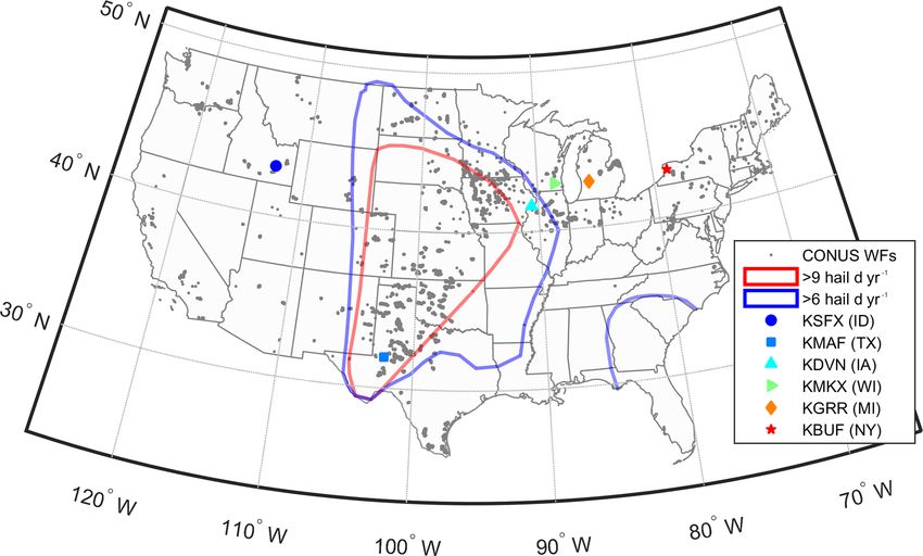
332                                                       F. Letson et al.: Precipitation climatology for wind turbine blade LEE

severe hail is almost certainly more common in the central          reached). Once the time to damage has been exceeded, ad-
US than in other areas of the world with substantial wind           ditional damage occurs as stress waves propagate from the
energy development (Prein and Holland, 2018). Further, the          impact sites into the composite and cause existing pits and
relationship linking damage to the frequency and severity of        cracks to grow, and there is a steady increase of material loss
hail varies substantially with the target. WTs present an inter-    with each additional impact (Cortés et al., 2017; Eisenberg
esting challenge in this context because they are large struc-      et al., 2018; Traphan et al., 2018). The number of impacts
tures and the blades are rotating, composite materials.             required to reach the threshold for surface fatigue failure is
   A key cause of the need for WT blade repairs is excess           a function of the droplet diameter and phase, the closing ve-
damage (i.e., material loss) on the leading edge (leading edge      locity, the strength of the material, and the pressure of the
erosion, LEE). LEE roughens WT blades, reducing lift and            impact. Hence, the material’s response to hail (solid hydrom-
electrical power production (Sareen et al., 2014; Gaudern,          eteors) may differ from that to collisions with liquid (rain)
2014). LEE causes an average of 1 %–5 % reduction in an-            droplets. For example, the maximum von Mises stress cre-
nual energy production (AEP) (Froese, 2018) and up to a 9 %         ated in the WT blade leading edge from a 10 mm diameter
reduction when delamination occurs (Schramm et al., 2017).          hailstone greatly exceeds that from a rain droplet of equiva-
Thus, excess LEE may be costing the industry tens of mil-           lent size and closing velocity due to differences in mass and
lions of dollars per year via lost revenue and/or increased         hardness (Keegan et al., 2013).
maintenance costs and poses a threat to achieving contin-              WT LEE is a developing area of research and uncertainty
uing wind energy cost reductions (Sareen et al., 2014). In          remains regarding the frequency and severity of the issue.
response to this issue a major industrial research consor-          Rates of LEE appear to be highly spatially variable due
tium from Europe (including DNV GL, Vestas and Siemens              to variations in WT operating conditions and the precipita-
Gamesa Renewable Energy) has recently (November 2018)               tion climate. Industrial experience has demonstrated that ex-
announced a new partnership (COBRA) focused on the anal-            posure to particularly harsh operating conditions can erode
ysis of mitigation measures for LEE including the devel-            coatings causing partial delamination after as little as 2–
opment of next-generation leading-edge protection systems           3 years (Rempel, 2012; Keegan et al., 2013). Elastomeric
(Durakovic, 2019).                                                  coatings can be applied for additional erosion resistance
   WT blades use composites (e.g., epoxy or polyester,              (Dalili et al., 2009; Valaker et al., 2015; Herring et al., 2019).
with reinforcing glass or carbon fibers) (Mishnaevsky Jr. et        However, the life of such coatings cannot be predicted ac-
al., 2017) coated to protect the blade structure by distribut-      curately (and is a function of UV exposure; Shokrieh and
ing and absorbing the energy from impacts (Brøndsted et             Bayat, 2007); they have a negative impact on blade aerody-
al., 2005). Thus, the leading edge actually comprises several       namics (Giguère and Selig, 1999) and their cost effectiveness
layers of the main structural composite material (and thick-        is uncertain (Dashtkar et al., 2019).
ening materials) plus coatings (Mishnaevsky Jr. et al., 2017).         The total installed capacity (IC) and rated capacity
Impact fatigue caused by collision with rain droplets and           (and physical dimensions) of WT being installed exhibited
hail stones is a primary cause of WT blade LEE (Bech et             marked growth in the USA over the last 20 years (Wiser and
al., 2018; Bartolomé and Teuwen, 2019; Zhang et al., 2015).         Bolinger, 2018; Wiser et al., 2016). Average WT blade length
Although rain droplets fall at only modest velocities (typi-        increased from < 4 m in 1985 to 32 m in 2005 and now ex-
cally ≤ 10 m s−1 , see details below), the tip of WT blades         ceeds 55 m (Wiser and Bolinger, 2018). Since the tip speed
rotate quickly (50–110 m s−1 ); thus the net closing velocity       increases with blade length, this tendency towards taller WTs
and kinetic energy transfer are large. Each precipitation im-       with longer blades exacerbates LEE potential. The increased
pact on the blade leading edge results in transient stresses        blade length and larger maintenance costs associated with
that are proportional to impact velocity (Preece, 1979; Slot        offshore wind turbines tend to make offshore wind farms
et al., 2015). The stress induced by individual high net col-       especially vulnerable to LEE. Based on previous research
lision impacts with hydrometeors may, in principle, exceed          the a priori expectation of this research is that excess LEE
the strength of the material. Estimates of the failure energy       is most likely on WTs deployed in environments with high
threshold of a composite structure vary widely (e.g., val-          rain intensities and hail frequencies, such as experienced in
ues of 72–140 J are given in Appleby-Thomas et al., 2011)           the Great Plains (the states of Texas, TX; Oklahoma, OK;
and may exceed 300 J for leading-edge thicknesses and hail-         Kansas, KS; Nebraska, NE; North and South Dakota, ND,
stone diameters > 20 mm (Kim and Kedward, 2000). How-               SD; Wyoming, WY; and Montana, MN; Fig. 1). LEE is likely
ever, conceptually the erosion of homogeneous materials is          to present a growing issue within the US wind industry as
most frequently considered using a three-stage model. Ini-          more and larger wind turbines with higher tip-speed ratios
tially there is an incubation period during which impacts oc-       are deployed (Amirzadeh et al., 2017a). The current average
cur but no visible damage is observed, although microstruc-         age of WTs in the US is 9 years (AWEA, 2019), and LEE
tural changes in the materials generate nucleation sites for        will be of greater concern as a larger number of WTs move
material removal, which commences when a threshold is               out of the typical 1- to 5-year warranty period (Bolinger and
reached (i.e., when some level of accumulated impacts is            Wiser, 2012; Brown, 2010).

Wind Energ. Sci., 5, 331–347, 2020                                                          www.wind-energ-sci.net/5/331/2020/
F. Letson et al.: Precipitation climatology for wind turbine blade LEE                                                          333

Table 1. The station code and locations of the six NWS dual-          based on a characterization of the kinetic energy exchange
polarization radars from which data are presented (listed from west   from rain and hail impacts on the blade leading edge. The
to east).                                                             procedure used in making these estimates is divided into two
                                                                      steps: the calculation of meteorological parameters (wind
        Station code   Latitude (N)   Longitude (E)    State          speed, rain and hail) at six wind farms, each located within
        KSFX             43.106          −112.686       ID            the observation area of a radar station, and then the calcula-
        KMAF             31.943          −102.189       TX            tion of blade impact frequencies and energy transfer based on
        KDVN             41.612           −90.581       IA            those meteorological parameters. Exact wind farm locations
        KMKX             42.968           −88.551       WI            and details are excluded from this paper under a nondisclo-
        KGRR             42.894           −85.545       MI            sure agreement (NDA).
        KBUF             42.949           −78.737       NY               The research reported herein leverages resources gener-
                                                                      ated from the upgraded National Weather Service (NWS)
                                                                      network of WSR-88D radar to dual polarization (completed
   Addressing the challenges posed by blade LEE and de-               in 2013; Seo et al., 2015; Crum et al., 1998) along with the
veloping mitigation options requires multi-scale and multi-           NOAA Weather and Climate Toolkit (WCT) (see details of
disciplinary research. Given the importance of precipitation          the data products and data volumes provided in Appendix A).
phase, size and intensity during WT operation to the poten-           These data represent a unique opportunity to characterize
tial for blade LEE, here we focus on developing a consis-             precipitation properties such as hail that are very challenging
tent and generalizable framework that can be applied to de-           to detect and to accurately characterize using in situ meth-
rive estimates of erosion-relevant atmospheric properties. We         ods or human observers (see discussion in Allen and Tippett,
present an objective, spatially consistent, robust and repeat-        2015, and details of radar operation in Kumjian, 2018). NWS
able framework that can be applied across CONUS and cru-              radars operate at elevation angles between 0.5 and 19.5◦ and
cially uses only noncommercial (i.e., publicly available) data.       an azimuthal resolution of 1◦ . Doppler and dual-polarization
The specific objectives of the research reported herein are as        data are publicly available at a resolution of 0.25 km up to a
follows:                                                              range of 300 km from each radar site (NOAA, 1991; Istok
                                                                      et al., 2009) (see description of the data provision in Kelle-
    1. to develop the workflow necessary to develop a proto-
                                                                      her et al., 2007, and an example of the NWS products given
       type radar-based erosion atlas;
                                                                      in Fig. 2). The temporal resolution of the data is typically
    2. to provide a first estimate of the spatial variability of      ∼ 5 min, but varies slightly with scanning mode: (1) clear-
       erosion potential across CONUS in regions where wind           air mode uses longer, 10 min scans to collect sufficient re-
       turbines are currently deployed (see Fig. 1);                  turn data during times of no precipitation when signal re-
                                                                      turn strength is relatively low; (2) precipitation mode is used
    3. to conduct an initial uncertainty propagation exercise to      when there is any precipitation detected in the scan area and
       illustrate how uncertainties in the input data propagate       uses a 6 min scan cycle; (3) storm mode is used when se-
       through the analysis workflow to influence erosion po-         vere or rapidly evolving storms are present and uses a 5 min
       tential estimates;                                             sampling interval, made possible by reducing the number of
    4. to describe the degree to which blade LEE is episodic          elevation angles used (NOAA, 2016a). Storm detection and
       and therefore amendable to the mitigation strategy pro-        tracking using radar is a complex and evolving science, but
       posed earlier in research from Denmark of WT cur-              in brief the NWS system uses an automated function which
       tailment during “highly erosive” periods. The efficacy         employs reflectivity from the current scan and storm cell lo-
       of this strategy is a function of (i) the wind speed           cation and vertically integrated liquid water (VIL) from the
       regime and joint probability distributions of erosive          previous scan (Johnson et al., 1998).
       events (heavy rain or hail) and power-producing wind              To illustrate the proposed analysis framework we use data
       speeds, (ii) the price of electricity supplied to the grid     from six NWS dual-polarization Doppler radar stations (see
       and (iii) O&M costs. A cost–benefit analysis based on          Fig. 1 and Table 1) collected over the period 2014–2018.
       conditions in Denmark suggested that the loss of rev-          These locations were chosen to represent gradients in hail
       enue from the curtailment of power production was              probability and precipitation amount in regions with rela-
       small compared to the economic benefits from enhanced          tively high wind turbine installed densities (Fig. 1). We em-
       blade lifetimes (Bech et al., 2018).                           ploy the framework in order to generate erosion climates for
                                                                      six wind farms operating in the scanned volume of the radars
                                                                      and located 35–75 km from the radar locations. The follow-
2    Data and methods                                                 ing radar data products are used (see also Appendix A):

A first estimate of precipitation-derived erosion potential at
sites across the USA as developed in the current work is

www.wind-energ-sci.net/5/331/2020/                                                           Wind Energ. Sci., 5, 331–347, 2020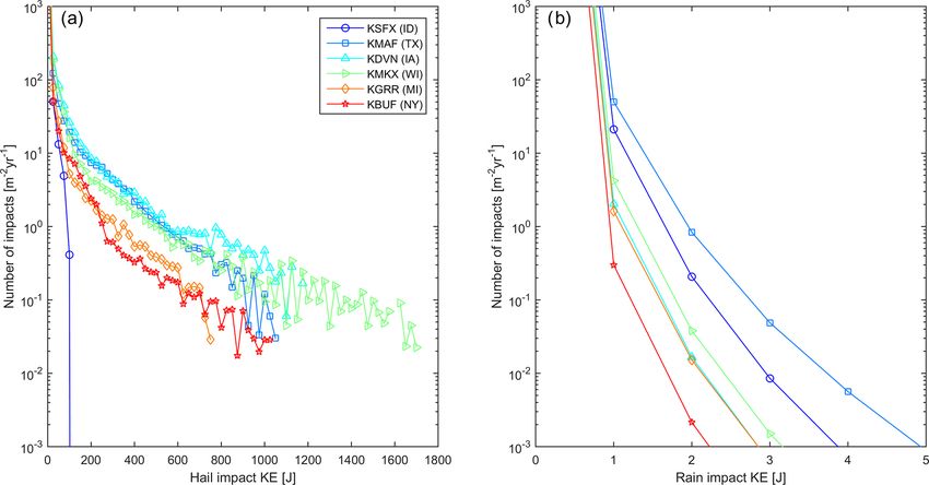
334                                                           F. Letson et al.: Precipitation climatology for wind turbine blade LEE

Figure 1. Locations of wind turbines as deployed at the end of 2017 according the USGS database (available from https://eerscmap.usgs.
gov/uswtdb/, last access: 15 January 2020; USGS, 2018) (grey dots), the NWS radar stations from which data are presented (see details in
Table 1) and areas of frequent hail occurrence. Areas with more than 9 hail days per year are outlined by the red contour, and those with more
than six are outlined by the blue contours (Cintineo et al., 2012).

  – Precipitation rate (N1P) is the precipitation rate in each
    radar cell in each ∼ 5 min period (expressed in units of
    millimeters per hour) as estimated from reflectivity.

  – Hybrid Hydrometer Classification (HHC), based on re-
    flectivity, temperature and dual-polarization variables,
    is an estimate of the most likely targets within the
    radar volume. While this is a derived product, classifi-
    cation algorithms and accuracy have improved with the
    widespread adoption of dual-polarization radar and the
    application of areal (rather than point-wise) techniques
    (NOAA, 2016b; Chandrasekar et al., 2013). The hy-
    drometeor types encoded in the NWS data product are
    dry snow, wet snow, crystals, big drops, rain (light and
    moderate), heavy rain, graupel and rain with hail.

  – In hail reports (NHI), maximum hail size (an estimate                Figure 2. Example of a single 5 min period of radar data from
    of the 75th percentile hail stone diameter, D75 ) and the            KSFX (ID; 8 August 2013, 22:37 UTC). The colors show the com-
    probability of hail are used to identify the occurrence              posite reflectivity (i.e., the maximum reflectivity from any of the
    and severity of hail events (see discussion in Witt et               elevation angles sampled by the NWS radar) in decibel reflectiv-
    al., 1998).                                                          ity (dBZ). The circles represent storm cells that are identified and
                                                                         tracked by the NWS detection algorithm; black circles are storms
  – Composite reflectivity (NCR) is the maximum reflectiv-               without hail, and red circles are those with hail.
    ity at any elevation angle measured in each radar cell.
    This is used here to characterize the spatial extent of
    hail events (i.e., reflectivity > 50 dBZ (decibel reflectiv-            Wind speeds, hydrometeor type and precipitation inten-
    ity), Witt et al., 1998).                                            sity for each nominal wind farm located within each radar-
                                                                         scanned area in each 5 min period are derived as follows.
  – Radial wind speeds from the 0.5 elevation angle are                     Precipitation intensity is characterized by rainfall rate
    computed from the Doppler shift (N0V) (Alpert and Ku-                (RR) in millimeters per hour, which is derived using radar
    mar, 2007).                                                          Z–R relationships (Wilson and Brandes, 1979) and reported

Wind Energ. Sci., 5, 331–347, 2020                                                                www.wind-energ-sci.net/5/331/2020/
F. Letson et al.: Precipitation climatology for wind turbine blade LEE 335
in the parameter precipitation rates (N1P) in all radar cells where θ is the difference in angle between the radar beam and
every ∼ 5 min. A spatial mean of all N1P values in all radar the direction of mean flow and Vmean is the mean wind speed
cells within 5 km of the wind farm centroid is used here. This at hub height. A least-squares fit of a sinusoid of this form is
rainfall rate is also used to derive the raindrop spectrum us- made to each wind speed scan (excluding cells which report a
ing the Marshall–Palmer distribution (Marshall and Palmer, zero wind speed) to estimate Vmean . The resulting wind speed
1948). In it the number of droplets above radius, R, per cubic is then used within the simple description of the blade rota-
meter of air (N , m−3 ) is given by tional speed as a function of hub-height wind speed as shown
in Fig 4c. This operational RPM (revolutions per minute)
N0 −3 R curve is based on long-term data provided from large oper-
N= e , (1)
3 ating WT arrays (under an NDA) and represents the mean
rotational speed across all WTs operating in these arrays as
where 3 = 8200 (RR)−0.21 (m−1 ), RR is the rainfall rate in
a function of the mean wind speed at hub height across the
millimeters per hour and N0 = 1.6×10⁷ m−4 ; see an example
arrays. The mean RPM decreases at wind speeds below the
rain droplet size distribution, expressed as dN/dR, for an RR
cut-out velocity (of 25 m s−1 ) due to some WTs rotating be-
of 25 mm h−1 in Fig. 3.
low their design RPM at very high wind speeds (near cut out)
Hail occurrence is characterized by a number of NWS
as reported in the SCADA (supervisory control and data ac-
radar-derived parameters, most of which are contained in the
quisition) data.
hail reports (NHI). Hail size and the probability of occur-
Once the hydrometeor type (rain or hail), hydrometeor
rence are conservatively estimated here, by taking the largest
size (which determines mass and terminal velocity) and wind
D75 value and hail probability reported for any storm cell
speed for a reporting period are known, hydrometeor impact
within 5 km of the nominal wind farm centroid (which will
energies for that period are calculated using the mass and
tend to bias both toward higher values). The spatial cover-
closing velocity for hydrometeors of each radius occurring
age of hail within that 5 km radius is determined by calcu-
in the period. For this analysis the terminal velocity for each
lating the fraction of radar cells in that area which have a
size of rain droplets is derived using (Stull, 2015)
composite reflectivity in excess of 50 dBZ. Hail size distri-
butions are relatively uncertain but are generally considered
ρ0
1/2
to be exponential up to a ceiling diameter (Auer, 1972; Lane Vt, rain = k R , (4)
ρair
et al., 2008). Herein the size distribution of hailstones is as-
sumed to follow (Cheng and English, 1983)
where R is the droplet radius (m), k = 220 m1/2 s−1 and ρ0
is air density at sea level (set to a constant of 1.25 kg m−3 ,
N(D) = 115λ3.63 e−λD , (2)
herein), ρair is air density at the altitude above sea level at
where D is the hailstone diameter (Cheng and English, which the rain droplet is crossing the rotor plane (see exam-
1983). This formulation is based on seven events sampled ple of Vt, rain in Fig. 3). The terminal velocity of hail stones
in Alberta, Canada, which covered a smaller diameter range is derived using (Stull, 2015)
than indicated by the radar products, but it has the advantage 1/2
that the distribution requires a single fitting parameter (λ) 8 |g| ρi
Vt, hail = R , (5)
and thus can be fully described using only D75 . As shown 3 CD ρair
by the example hail distribution (expressed in dN/dR) for
where R is radius of the hailstone (m), ρi is the density of
D75 = 25 mm and λ = 0.053 mm−1 (Fig. 3), the slope of
ice (set to a constant of 900 kg m−3 herein) and ρair is air
the hydrometeor diameter is considerably shallower than for
density at the altitude at which the hail is falling. CD = 0.55
rain droplets as described using Marshall–Palmer. In order to
is the drag coefficient (Stull, 2015) (see example of Vt, hail in
avoid the occurrence of extremely large hailstones, we trun-
Fig. 3).
cate the distribution to include diameters up to 2 times the
Closing velocity, Vc , as a function of hydrometeor type
radar-estimated 75th percentile hail stone diameter (D75 ).
and diameter (D) is calculated from wind speed, Vmean , ro-
The presence of such a hail size ceiling is consistent with
tor speed, Vr (calculated from wind speed and RPM curve),
previous observations (Auer, 1972).
terminal velocity, Vt , and blade position, φ(t). Vr as derived
Wind speeds from radar have been previously used for
here represents the linear speed of the blade tip due to rota-
numerical wind resource verification (Salonen et al., 2011).
tion, as this will lead to conservative estimates of impact en-
Wind speeds at a typical wind turbine hub height of approx-
ergy. Local blade speeds increase linearly with distance from
imately 80 m are derived using the radial wind speeds from
the hub, so both the frequency and the energy of impacts is at
the 0.5◦ elevation angle scan at a distance of 8 km (±0.5 km)
a maximum near the blade tip, where blades are particularly
range from the radar station using an assumption of uniform
susceptible to erosion (Keegan et al., 2013).
flow from
h i1/2
2
Vradial (θ ) = Vmean cos(θ ), (3) Vc (D, t) = Vmean + (Vr + Vt (D) · cos (φ(t)))2 . (6)
www.wind-energ-sci.net/5/331/2020/ Wind Energ. Sci., 5, 331–347, 2020336 F. Letson et al.: Precipitation climatology for wind turbine blade LEE
The impact rate (I ) on the blade leading edge as a function
of hydrometeor type and size is calculated from the number
density of the hydrometeors of a given diameter (N(D)) and
the closing velocity:
I (D, t) = N (D) · Vc (D, t) . (7)
The assumption that all falling rain droplets will impact the
blade is made on the basis of evidence that only droplets with
diameters below 0.2 mm have insufficient inertia to be de-
flected from the blade by streamline deformation (Eisenberg
et al., 2018). The maximum kinetic energy transferred to the
blade from the hydrometeors is then computed for each hy-
drometeor type and diameter using the following approxima-
tion:
1
EK (D, t) = m(D) · Vc (D, t)2 , (8) Figure 3. Example of the hydrometeor number density (dN/dR;
2 number of droplets per meter cubed of air per millimeter of radius
where m(D) is the mass of the hydrometeors of a given di- increment) for a precipitation rate of 25 mm h−1 for rain droplets (as
ameter. described using the Marshall–Palmer size distribution) and for hail
stones (for D75 of 25 mm and λ = 0.053 mm−1 ) (left axis). Note:
The total kinetic energy of impacts over a time interval, T ,
the λ value employed (λ = 0.053 mm−1 ) differs from the range (λ:
associated with hydrometeors of diameter, D, is given by: 0.1 to 2 mm−1 ) used by Cheng and English (1983) for the seven
Z t0 +T events they sampled and thus corresponds to a larger maximum hail
EK, T (D) = I (D, t) · EK (D, t) dt, (9) size. Hydrometeor terminal velocities of hail and rain are shown by
t0 radius on the right axis.
where dt is the time interval at which the radar measurements
are available (5 min).
percentile value at KMKX (18 mm h−1 ) and the Vmean is set
The radar-estimated probability of hail and the geographic
to the mean value (12.8 m s−1 ) during heavy rainfall (i.e., RR
extent of hail fall are both treated probabilistically with re-
within 10 % of the 99th percentile value at KMKX).
spect to the number of expected hail impacts on any partic-
Uncertainties in radar-derived hail sizes are less well char-
ular wind turbine within the wind farm. The number of ex-
acterized than for Vmean and RR. For RR the range of ±50 %
pected impacts at each kinetic energy are multiplied by two
is inclusive of previously published uncertainties, under-
factors representing two effects: (1) the probability of hail be-
standing that those uncertainties are a function of spatial res-
ing associated with the storm in question, as estimated by the
olution, RR and the radar processing algorithm (Seo and Kra-
radar hail detection algorithm, and (2) the fraction of radar
jewski, 2010; Seo et al., 2015). Wind speed uncertainty (as
cells within 5 km of the wind farm centroid which have a
quantified using RMSE) for an elevation angle of 0.5◦ is ap-
composite reflectivity of > 50 dBZ, the range commonly as-
proximately ±3.4 m s−1 (Fast et al., 2008), and thus for a
sociated with hail.
wind speed of 12.8 m s−1 a ±50 % variation is fully inclu-
NWS radar products have been subject to extensive prod-
sive of the estimated wind speed error.
uct development efforts and a wide range of evaluation ex-
ercises (Cunha et al., 2015; Villarini and Krajewski, 2010;
Straka et al., 2000) but are nevertheless associated with mea- 3 Results
surement uncertainties, as are the approximations applied
herein to derive terminal fall velocities and kinetic energy Key aspects of the erosion-relevant radar-derived atmo-
transfer. To provide a first assessment of how these uncer- spheric properties at the six locations are summarized in
tainties in input data propagate through the analysis frame- Fig. 4. Consistent with previous precipitation climatologies,
work and thus impact derived kinetic energy exchange, each there are marked spatial gradients in the annual total and pre-
of three key parameters of the erosion potential are perturbed cipitation intensity (RR, Fig. 4a) (Prat and Nelson, 2015).
from 50 % to 150 % of observed values during two exam- Precipitation rates of < 5 mm h−1 are common at all sites;
ple periods of comparatively high erosion potential. The first RRs of 20 mm h−1 are experienced at all locations, but only
case represents a period of large hail. In this analysis D75 is the site in Texas (KMAF) exhibits any occurrence of rain-
set to the 99th percentile D75 at KMKX (WI) (42 mm) and fall intensity in excess of 35 mm h−1 . Using a damage rate
Vmean is set to 11.3 m s−1 (i.e., the mean wind speed condi- of 3 × 10⁻⁵ s−1 for an RR of 20 mm h−1 and a closing ve-
tionally sampled by ±10 % of D75 = 42 mm). In the second, locity of 120 m s−1 (Eisenberg et al., 2018), the frequency of
a heavy rain event is considered. The RR is set to the 99th RR of 20 mm h−1 at the site in Texas is such that it would
Wind Energ. Sci., 5, 331–347, 2020 www.wind-energ-sci.net/5/331/2020/F. Letson et al.: Precipitation climatology for wind turbine blade LEE 337
accumulate ∼ 0.6 of impact necessary to reach the transition Table 2. Mean wind speeds close to WT HH from each radar: the
threshold from the incubation region to material loss over a long-term mean, Vmean , the mean during times of precipitation, Vp ,
25-year period. and the mean during times of no precipitation Vnp .
At most sites, snow and ice occur at rates at least 1 or-
der of magnitude less frequent than rain. The exception is Station code Mean wind speeds (m s−1 )
the site in Idaho (KSFX) (Fig. 4d). At each of the six loca- Vmean Vp Vnp
tions, there are fewer than forty 5 min hail periods per year.
Consistent with expectations and previous research (Cinti- KSFX (ID) 5.8 5.9 5.7
neo et al., 2012), while hail events occur at all six sites, KMAF (TX) 5.9 6.7 5.8
KDVN (IA) 10.0 11.1 9.8
hail frequency and severe hail events (with maximum hail
KMKX (WI) 8.8 10.2 8.7
sizes > 25 mm) are substantially more frequent at the nom-
KGRR (MI) 8.6 12.3 8.5
inal wind farm locations in Texas, Illinois and Wisconsin KBUF (NY) 9.2 10.9 9.0
(radar codes: KMAF, KDVN and KMKX) (Fig. 4b). The de-
rived frequency distributions of wind speed close to wind
turbine hub heights (WT HHs) exhibit a high frequency of
wind speeds above typical wind turbine cut-in speeds and
are particularly right-skewed at the site in Iowa (Fig. 4c). tent with the precipitation climatology summarized in Fig. 4b
The mean annual wind speed near nominal WT HH is lowest and the high frequency of wind speeds associated with high
at KSFX (ID), where it is ≈ 5.9 m s−1 . Wind speeds range WT RPM (Fig. 4c). At these three sites some events (5 min
from 8.6 to 10 m s−1 at KGRR (MI), KMKX (WI), KBUF periods) exhibit kinetic energy of transfer from hail in ex-
(NY) and KDVN (IA) (Table 2). The wind speed distribu- cess of 300 J (Fig. 5a). Although these events have a low
tions at these five of the six locations exhibit relatively good probability (less than 1 m−2 yr−1 ), they may thus be suffi-
qualitative agreement with a priori expectations (see wind cient to cause damage to blade coatings in isolation from
resource maps available at https://windexchange.energy.gov/ the effects of the cumulative fatigue (Appleby-Thomas et
maps-data/324, last access: 15 January 2020) and estimates al., 2011; Kim and Kedward, 2000). Conversely, individual
from simulations for 2002–2016 with the Weather Research rain impacts rarely exceed 5.2 J at any site. The probabil-
and Forecasting model (Pryor et al., 2018) for 12 km grid ity of exceeding this impact kinetic energy threshold over
cells containing the nominal wind field locations that indi- a square meter of blade leading edge is less that 10−3 yr−1
cate mean annual wind speeds of 6.5 m s−1 at KSFX (ID) and (Fig. 5b). Thus, hail dominates the annualized cumulative ki-
8.4–9.0 m s−1 (KGRR (MI), KMKX (WI), KBUF (NY) and netic energy of transfer to each square meter of the blades at
KDVN (IA)). However, wind speeds derived from radar ob- all sites (Fig. 6). Indeed, at all sites, despite the low proba-
servations from KMAF (TX) are relatively low (mean value bility of hail relative to rain (cf. Fig. 4a and b), total annual
of 5.9 m s−1 ) and exhibit a relatively low frequency of ob- kinetic energy transfer from hail exceeds that from rain by
servations above 13 m s−1 (2.2 %). This negative bias (of at least 2 orders of magnitude (Fig. 6). The lowest cumula-
> 1 m s−1 in the mean relative to the resource map and WRF tive kinetic energy transfer is projected for the nominal wind
model output) from the Texas site will tend to lead to lower farm sites in Idaho (KSFX), New York state (KBUF) and
RPM values and hence blade tip speeds and thus a negative Michigan (KGRR). Conversely, values are highest for Texas
bias in kinetic energy transfer at this location. Wind speed (KMAF), Iowa (KDVN) and Wisconsin (KMKX). This is
distributions during precipitation and no-precipitation peri- consistent with previous characterizations of hail frequency,
ods are qualitatively similar at all six locations. Modal values which show hail fall to be most common in the Great Plains
are within ±1.2 m s−1 , but the distributions are heavier-tailed and much less frequent west of 105◦ W (Fig. 1) (Cintineo et
at all sites during precipitation periods. Mean wind speeds al., 2012; Allen and Tippett, 2015).
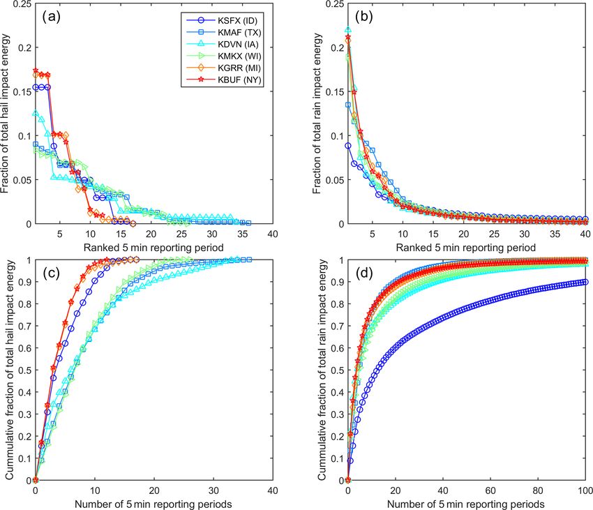
during precipitation are 0.2–3.8 m s−1 higher at the six loca- Figure 7 illustrates that only a very small fraction of 5 min
tions than during times of no precipitation (Table 2). periods dominate kinetic energy transfer to the blades from
Given the exponential dependence of hailstone and rain both hail and rain. At all sites over 80 % of rain-induced ki-
droplet size on precipitation intensity and the accumulated netic energy transfer occurs in the top eighty 5 min periods
damage therefrom (Eisenberg et al., 2018), the distributions per year. Indeed, at all but the site in Idaho (KSFX) over half
of kinetic energy transfer from the two hydrometeor types of the total rain-induced kinetic energy transfer to the blade
at all sites are heavy-tailed. Further, the probability distribu- occurs in only twenty 5 min periods in a year. The proba-
tions of each 5 min estimate of kinetic energy transfer (Fig. 5) bility distribution of hail-induced kinetic energy transfer is
and total annual kinetic energy transfer (Fig. 6) indicate even more heavy-tailed with 90 % of the cumulative kinetic
marked differences between the sites and between the two energy transfer to the blades from hail occurring in fewer
hydrometeor types. Extremely high hail kinetic energies are than twenty-five 5 min periods per year at all sites. Thus, few
most frequently projected for sites in Texas (KMAF), Iowa events dominate the annual total accumulated impact dam-
(KDVN) and Wisconsin (KMKX) (Fig. 5a). This is consis- age.
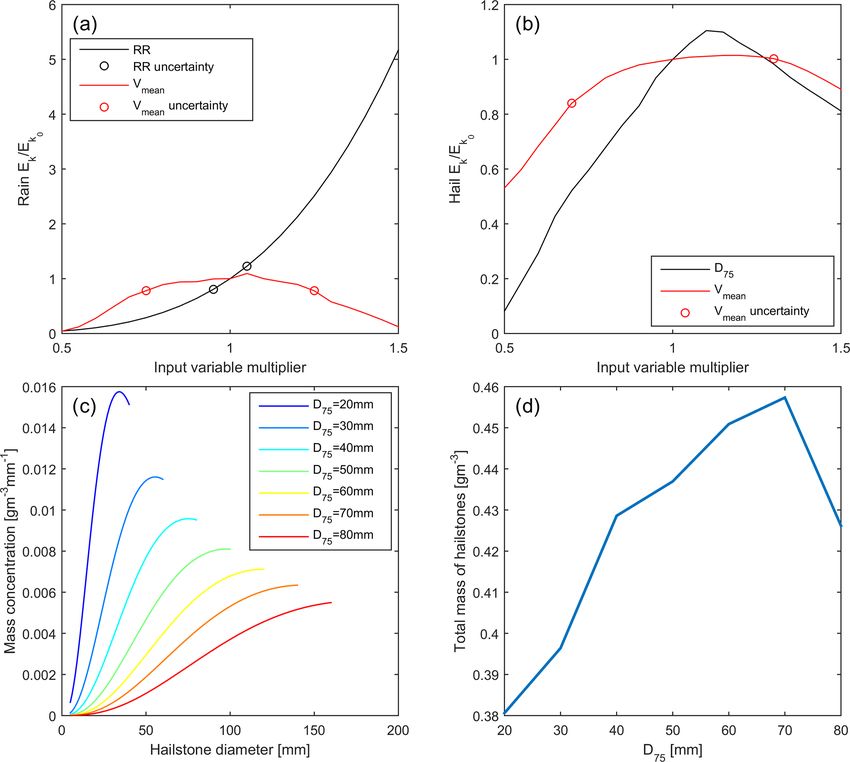
www.wind-energ-sci.net/5/331/2020/ Wind Energ. Sci., 5, 331–347, 2020338 F. Letson et al.: Precipitation climatology for wind turbine blade LEE Figure 4. Precipitation and wind speed climates from radar data (see locations in Fig. 1). (a) Mean annual number of 5 min periods of each RR intensity class (discretized in 5 mm h−1 intervals). (b) Mean annual number of 5 min periods with maximum hail sizes (D75 ) (discretized in 5 mm intervals). (c) Wind speed distributions for all 5 min periods (discretized in 2 m s−1 intervals). The black line in this frame shows the WT RPM curve as a function of wind speed (WTG RPM, right axis) (d). Occurrence of NWS radar hydrometeor classifications for each nominal wind farm shown as the fraction of radar cells in each class during all periods with RR > 1 mm h−1 . Illustrative examples of uncertainties in impact kinetic en- of hail (D75 = 42 mm and Vmean = 11.3 m s−1 ), impact ki- ergy due to radar observational uncertainties in Vmean , RR netic energy varies by ±20 % for a ±50 % variation in Vmean and D75 are shown in Fig. 8. For the representative 5 min and D75 (Fig. 8b). Impact kinetic energy actually decreases period of heavy rain, a variation of RR ± 50 % is associated as D75 exceeds 120 % of the nominal value (D75 = 42 mm) with a ±15 % variation in kinetic energy of impact (Fig. 8a). (Fig. 8b). This decrease is explained by the interaction of the Increases or decreases in mean wind speed by 4.2 m s−1 (the single parameter exponential hail size distribution (Fig. 4c) upper end of wind speed uncertainty observed in previous and the applied hail diameter ceiling. As D75 increases the work for an elevation angle of 0.5◦ ) (Fast et al., 2008) are truncation of the upper tail of the hail distribution (Fig. 8c) shown to decrease kinetic energy, since rotor speed decreases means the total modeled mass of hail per unit volume de- for wind speeds below or significantly above the rated wind creases (Fig. 8d). speed of the turbines (Fig. 4c). For a representative period Wind Energ. Sci., 5, 331–347, 2020 www.wind-energ-sci.net/5/331/2020/
F. Letson et al.: Precipitation climatology for wind turbine blade LEE                                                              339

Figure 5. Histograms of kinetic energy of hydrometeor impacts. Annual number of (a) hail and (b) rain impacts per square meter of blade
leading edge as a function of impact kinetic energy. The y axis in panel (b) has been truncated to a maximum value of 1000 yr−1 .

                                                                        though the data volumes are not trivial (see Appendix A),
                                                                        this analysis framework could be applied to NWS radar data
                                                                        to estimate LEE potential at any arbitrary site in CONUS
                                                                        and/or applied to data from other national dual-polarization
                                                                        radar networks for other regions of the world. For example,
                                                                        the Network of European Meteorological Services (EUMET-
                                                                        NET) operates over 200 radars many of which have been up-
                                                                        graded to dual polarization (Saltikoff et al., 2018). The tool
                                                                        proposed here could be used to provide a first assessment
                                                                        of the erosion climate in which a given sited turbine may
                                                                        operate. It thus provides an important first step towards en-
                                                                        abling an assessment of the threat of excessive precipitation-
                                                                        induced LEE in a given deployment environment and the cost
                                                                        effectiveness of options to reduce the likelihood of premature
                                                                        blade damage.
                                                                            The actual likelihood of excess WT LEE and blade dam-
                                                                        age in any environment is not only a function of the pre-
                                                                        cipitation and wind climate but also of the WT dimensions,
                                                                        materials used in the blade coatings and the coating thick-
Figure 6. Total annual kinetic energy (EK ) per square meter of         ness (Eisenberg et al., 2018; Slot et al., 2015), the presence
blade leading edge from rain and hail impacts at each location.         of existing microstructural defects (Evans et al., 1980) due
                                                                        to manufacturing defects and damage during transportation
                                                                        (Keegan et al., 2013; Nelson et al., 2017), and other aspects
4   Conclusions                                                         of the operating environment (including thermal fatigue and
                                                                        the occurrence of icing; Slot et al., 2015).
A robust and flexible framework has been developed and                      The preliminary estimates of erosion potential and the par-
presented for generating an observationally constrained geo-            titioning between liquid precipitation and hail are naturally
referenced assessment of precipitation-induced wind turbine             subject to limitations including, in likely order of importance,
blade leading edge erosion potential. The approach elabo-               the following:
rated herein is naturally subject to a range of uncertainties but
is automated, objective, repeatable and predicated on pub-                 – the relatively short duration of time for which the dual-
licly available data available from across most of the conti-                polarization radar products are available. The upgrade
nental US. Further, the modular structure means it is flexible               of the NWS radar network to dual polarization was
to use with different assumptions and/or data streams. Al-                   completed in April 2013; thus only the complete years

www.wind-energ-sci.net/5/331/2020/                                                               Wind Energ. Sci., 5, 331–347, 2020
340 F. Letson et al.: Precipitation climatology for wind turbine blade LEE
Figure 7. Contributions of the most intense precipitation events to annual total kinetic energy from hydrometeor impacts. (a) Contribution
of the top forty 5 min periods of hail as a fraction of the annual total kinetic energy of hail impacts. (b) Contribution of the top forty 5 min
periods of rain as a fraction of the annual total kinetic energy of rain impacts. Cumulative fraction of annual impact kinetic energy from the
top X (c) hail events and (d) rain events, where X is set to 40 for hail because no site exhibits more than 36 events per year and is truncated
to 100 for rain.
of 2014–2018 (inclusive) were available for analysis. with previous estimates of wind climates, values for the
Given the large interannual variability in precipitation location in Texas are negatively biased. This likely re-
climates, this is too short to build a comprehensive cli- sults in a negative bias in kinetic energy transfer for this
matology (Karl et al., 1995; Prein and Holland, 2018). site.
Any geospatial depiction of the potential precipitation
erosion climate will vary according to the precise data – assumptions regarding the size distribution, occurrence
period used to compute the climatology and may evolve and terminal velocities of hail (Dessens et al., 2015;
as a result of climate non-stationarity altering aspects Allen et al., 2017; Heymsfield et al., 2014). The evo-
of the precipitation climate (e.g., the probability of hail, lution of the NWS radar network to dual polarization
Brimelow et al., 2017, and rainfall intensity, Easterling provides an unprecedented opportunity for spatial es-
et al., 2000). timates of hail presence and size in clouds (Kumjian
et al., 2018). However, hail production is a complex
– the applicability of the radar-derived wind speed es- and incompletely understood phenomenon (Dennis and
timates to derive wind turbine blade rotational speed. Kumjian, 2017; Blair et al., 2017; Pruppacher and Klett,
There are considerable challenges to line-of-sight wind 2010). There are substantial event-to-event variations in
retrievals from radar (Fast et al., 2008). The approach the size distribution and density of hail stones (Heyms-
adopted herein assumes a uniform wind flow pattern to field et al., 2014), in the presence of solid-phase hy-
derive the wind speeds at the nominal wind turbine hub drometeors in clouds (as detected by radar) and the oc-
height, which may not be realized. As described above, currence of hail at the ground (Kumjian et al., 2019).
while the wind speed climates at five of the six loca- Estimates of hail occurrence, size distribution and ter-
tions considered exhibited relatively good agreement minal fall velocity presented herein are likely conserva-
Wind Energ. Sci., 5, 331–347, 2020 www.wind-energ-sci.net/5/331/2020/F. Letson et al.: Precipitation climatology for wind turbine blade LEE 341
Figure 8. Sensitivities of rain (a) and hail (b) impact kinetic energies in one 5 min period to the application of ±50 % uncertainties on
the input parameters; wind speed (Vmean ) and precipitation intensity (RR) or hail diameter (D75 ). Circles represent reported uncertainties
in radar retrievals of wind speed (Fast et al., 2008) and rainfall rate (see Table 1 in Seo and Krajewski, 2010). (c) Mass concentrations of
hailstones per cubic meter of air (expressed as dM/dD) associated with a range of D75 values as a function of hailstone diameter. (d) Total
hail mass (in grams) per cubic meter of air as a function of D75 .
tive (i.e., upper bounds on true values), and thus LEE Future work could address and reduce these uncertainties
may be overestimated. and adapt this approach to examine different wind turbines
(by applying a different RPM curve) and/or to assimilate dif-
– assumptions regarding the size distribution of rain ferent atmospheric data and/or incorporate more explicit as-
droplets. Most observational studies indicate an ex- pects of material response. In this analysis we have chosen
ponential form (Uijlenhoet, 2001), and the Marshall– to focus on an energetic approach in which we compute the
Palmer distribution is the most widely applied. How- accumulated kinetic energy transmitted to the blade leading
ever, a range of different forms have been proposed to edge instead of using approaches based on the waterhammer
describe the size spectrum of rain droplets (dN/dR) in- equation that seek to compute the impact pressure and ma-
cluding gamma (Ulbrich, 1983) and lognormal (Fein- terial response to the resulting Rayleigh, shear and compres-
gold and Levin, 1986), an alternative exponential form sion waves (that are assumed to act independently of each
(Best, 1950), and more complex non-parametric forms individual impact) (Slot et al., 2015; Dashtkar et al., 2019).
(Morrison et al., 2019). There is also evidence that It is important to reiterate that the approach adopted here, i.e.,
droplet size distributions may exhibit a functional de- to compute the maximum total kinetic energy transferred to
pendence on near-surface wind speed (Testik and Pei, the blade, which is used here as a proxy for the erosion po-
2017). tential, represents the upper bound on actual kinetic energy
transfer since it employs a closing velocity characteristic for
– assumptions applied in deriving precipitation intensity the tip of WT rotors, assumes all falling hydrometeors im-
and other precipitation properties from radar. Notable pact the blade, and neglects energy loss during the transfer,
event-to-event variations in the applicability of Z–R re- “splash” and bounce of hydrometeors. There are more com-
lationships have been reported during rain (Uijlenhoet, plex frameworks that can be applied to simulate the pressure
2001; Villarini and Krajewski, 2010). and transient stresses on the blade coatings (Mishnaevsky Jr.,
www.wind-energ-sci.net/5/331/2020/ Wind Energ. Sci., 5, 331–347, 2020342 F. Letson et al.: Precipitation climatology for wind turbine blade LEE 2019) and impingement erosion (Amirzadeh et al., 2017a, b). A model of the blade response to precipitation impacts could be incorporated within the analysis framework to examine the probability and time to exceed the (cumulative) failure threshold energy (Fiore et al., 2015). This work suggests the dominance of hail as a damage vec- tor for WT blades at all of the sites studied here. This is con- sistent with indications that deep convection and hail are par- ticularly common in the central US (Cintineo et al., 2012) and indications of large geographic variability in hail fre- quency (Ni et al., 2017). This finding emphasizes the key importance of efforts to build and enhance hail climatologies (Allen et al., 2015; Gagne et al., 2019) with applications in a wide range of industries (from insurance to renewable en- ergy). The dominance of hail as a damage vector and the im- portance of a relatively small number of 5 min periods to total annual kinetic energy transfer from rain adds credence to the proposal that blade LEE could be greatly reduced by operat- ing erosion-safe turbine control (Bech et al., 2018), wherein the WTs are curtailed during periods with extreme precip- itation (very heavy rain or the occurrence of hail) without substantial loss of income. Wind Energ. Sci., 5, 331–347, 2020 www.wind-energ-sci.net/5/331/2020/
F. Letson et al.: Precipitation climatology for wind turbine blade LEE                                 343

Appendix A

The workflow, NWS radar data products and data volumes
necessary for the components of the precipitation erosion cli-
mate are as follows:
 1. Download daily .tar archives of NEXRAD polarized
    Doppler radar data using ftp from the data repos-
    itory hosted at https://www.ncdc.noaa.gov/nexradinv/
    (last access: 7 January 2019; NOAA, 1991). These tar
    archives contain all NEXRAD level 2 and 3 data and
    data products at 5 min intervals in binary NEXRAD for-
    mat. The 365 daily tar comprise 60–100 GB per station
    per year (PSPY).
 2. Preprocessing:

      a. Extract precipitation rates (N1P) and hail reports
         (NHI) files from each daily tar file.
      b. Import raw files into NOAA Weather and Climate
         Toolkit (https://www.ncdc.noaa.gov/wct/, 15 Jan-
         uary 2020; NOAA NCEI, 2020a), translate N1P,
         N0V and NHI files into netcdf and .csv, file sizes
         and numbers:
           - hydrometeor classification (HHC) raw files
             (32 000 to 70 000 files PSPY, 124–180 MB
             PSPY)
           - NHI csv files (12 000 to 137 000 files PSPY, to-
             taling 25–190 MB PSPY)
           - N1P raw files (68 000 to 90 000 files PSPY, to-
             taling 600–900 MB PSPY)
           - N1P netcdf files (130 000 to 150 000 files PSPY,
             totaling 240–290 GB PSPY)
           - base wind speed (N0V) raw files (40 000 to
             60 000 files PSPY, totaling 35–45 GB PSPY)
           - N0V netcdf files (40 000 to 60 000 files PSPY,
             totaling 900–1100 MB PSPY).
  Subsequent data analysis is conducted within MATLAB.

www.wind-energ-sci.net/5/331/2020/                                       Wind Energ. Sci., 5, 331–347, 2020
344 F. Letson et al.: Precipitation climatology for wind turbine blade LEE
Data availability. The USGS Wind Turbine Database used in References
Fig. 1 is available for download from https://eerscmap.usgs.gov/
uswtdb/ (last access: 15 January 2020; USGS, 2018). The NOAA Allen, J. T. and Tippett, M. K.: The characteristics of United States
Weather and Climate Toolkit (WCT) is a free, platform-independent hail reports: 1955–2014, E-Journal of Severe Storms Meteorol-
Java-based software tool distributed by NOAA’s National Cen- ogy, 10, 1–31, 2015.
ters for Environmental Information (NOAA NCEI, 2020a) (down- Allen, J. T., Tippett, M. K., and Sobel, A. H.: An empirical model
load is available from https://www.ncdc.noaa.gov/wct/, last access: relating US monthly hail occurrence to large-scale meteorologi-
15 January 2020). The NWS radar data are available from https: cal environment, J. Adv. Model. Earth Sy., 7, 226–243, 2015.
//www.ncdc.noaa.gov/data-access/radar-data (last access: 15 Jan- Allen, J. T., Tippett, M. K., Kaheil, Y., Sobel, A. H., Lepore, C.,
uary 2020; NOAA NCEI, 2020b). Nong, S., and Muehlbauer, A.: An extreme value model for US
hail size, Mon. Weather Rev., 145, 4501–4519, 2017.
Alpert, J. C. and Kumar, V. K.: Radial wind super-obs from the
Author contributions. SCP and RJB jointly designed the project WSR-88D radars in the NCEP operational assimilation system,
and obtained the funding and computing resources for the project. Mon. Weather Rev., 135, 1090–1109, 2007.
FL conducted the majority of the data analysis and developed the Amirzadeh, B., Louhghalam, A., Raessi, M., and Tootkaboni, M.:
figures with input from SCP and RJB. All contributed to writing the A computational framework for the analysis of rain-induced ero-
paper. sion in wind turbine blades, part I: Stochastic rain texture model
and drop impact simulations, J. Wind Eng. Ind. Aerod., 163, 33–
43, 2017a.
Amirzadeh, B., Louhghalam, A., Raessi, M., and Tootkaboni, M.:
Competing interests. The authors declare that they have no con-
A computational framework for the analysis of rain-induced ero-
flict of interest.
sion in wind turbine blades, part II: Drop impact-induced stresses
and blade coating fatigue life, J. Wind Eng. Ind. Aerod., 163, 44–
54, 2017b.
Special issue statement. This article is part of the special issue
Appleby-Thomas, G. J., Hazell, P. J., and Dahini, G.: On the re-
“Wind Energy Science Conference 2019”. It is a result of the Wind sponse of two commercially-important CFRP structures to mul-
Energy Science Conference 2019, Cork, Ireland, 17–20 June 2019. tiple ice impacts, Composite Structures, 93, 2619–2627, 2011.
Auer, A. H.: Distribution of graupel and hail with size, Mon.
Weather Rev., 100, 325–328, 1972.
Acknowledgements. This research was funded by the US De- AWEA: US wind industry annual market report year end-
partment of Energy (DE-SC0016438 and DE-SC0016605) and Cor- ing 2018, American Wind Energy Association, Wash-
nell University’s Atkinson Center for a Sustainable Future (ACSF- ington, DC, USA, available at: https://www.awea.
sp2279-2018). It was enabled by access to computational resources org/resources/publications-and-reports/market-reports/
supported via the NSF Extreme Science and Engineering Dis- 2018-u-s-wind-industry-market-reports (last access: 15 January
covery Environment (XSEDE) (award TG-ATM170024) and ACI- 2020), 2019.
1541215. The authors gratefully acknowledge the scientists and Bartolomé, L. and Teuwen, J.: Prospective challenges in the experi-
technicians of the National Weather Service for their work in real- mentation of the rain erosion on the leading edge of wind turbine
izing the dual-polarization radar network and making the data pub- blades, Wind Energy, 22, 140–151, 2019.
licly available. We appreciate the contributions of our two peer re- Bech, J. I., Hasager, C. B., and Bak, C.: Extending the life of
viewers in making this a clearer, more effective paper. wind turbine blade leading edges by reducing the tip speed dur-
ing extreme precipitation events, Wind Energ. Sci., 3, 729–748,
https://doi.org/10.5194/wes-3-729-2018, 2018.
Financial support. This research has been supported by the Best, A.: The size distribution of raindrops, Q. J. Roy. Meteor. Soc.,
U.S. Department of Energy (grant nos. DE-SC0016438 and DE- 76, 16–36, 1950.
SC0016605) and the Atkinson Center for a Sustainable Future Blair, S. F., Laflin, J. M., Cavanaugh, D. E., Sanders, K. J., Cur-
(grant no. ACSF-sp2279-2018). rens, S. R., Pullin, J. I., Cooper, D. T., Deroche, D. R., Leighton,
J. W., and Fritchie, R. V.: High-resolution hail observations: Im-
plications for NWS warning operations, Weather Forecast., 32,
Review statement. This paper was edited by Julio J. Melero and 1101–1119, 2017.
reviewed by two anonymous referees. Bolinger, M. and Wiser, R.: Understanding wind turbine price
trends in the US over the past decade, Energ. Policy, 42, 628–
641, 2012.
Brimelow, J. C., Burrows, W. R., and Hanesiak, J. M.: The chang-
ing hail threat over North America in response to anthropogenic
climate change, Nat. Clim. Change, 7, 516–522, 2017.
Brøndsted, P., Lilholt, H., and Lystrup, A.: Composite materials for
wind power turbine blades, Annu. Rev. Mater. Res., 35, 505–538,
2005.
Wind Energ. Sci., 5, 331–347, 2020 www.wind-energ-sci.net/5/331/2020/F. Letson et al.: Precipitation climatology for wind turbine blade LEE 345
Brown, M.: Turbine servicing act before the warranty is over, Wind Evans, A., Ito, Y., and Rosenblatt, M.: Impact damage thresholds
Power Monthly, 989458, 10 March 2010. in brittle materials impacted by water drops, J. Appl. Phys., 51,
Brown, T. M., Pogorzelski, W. H., and Giammanco, I. M.: Evalu- 2473–2482, 1980.
ating hail damage using property insurance claims data, Weather Fast, J. D., Newsom, R. K., Allwine, K. J., Xu, Q., Zhang, P.,
Clim. Soc., 7, 197–210, 2015 Copeland, J., and Sun, J.: An evaluation of two NEXRAD wind
Carroll, J., McDonald, A., and McMillan, D.: Failure rate, repair retrieval methodologies and their use in atmospheric dispersion
time and unscheduled O&M cost analysis of offshore wind tur- models, J. Appl. Meteorol. Clim., 47, 2351–2371, 2008.
bines, Wind Energy, 19, 1107–1119, 2016. Feingold, G. and Levin, Z.: The lognormal fit to raindrop spectra
Chandrasekar, V., Keränen, R., Lim, S., and Moisseev, D.: Recent from frontal convective clouds in Israel, J. Clim. Appl. Meteorol.,
advances in classification of observations from dual polarization 25, 1346–1363, 1986.
weather radars, Atmos. Res., 119, 97–111, 2013. Fiore, G., Camarinha Fujiwara, G. E., and Selig, M. S.: A damage
Changnon, S. A.: Data and approaches for determining hail risk in assessment for wind turbine blades from heavy atmospheric par-
the contiguous United States, J. Appl. Meteorol., 38, 1730–1739, ticles, in: 53rd AIAA Aerospace Sciences Meeting, 5–9 January
1999. 2015, Kissimmee, Florida, AIAA SciTech, 22 pp., 2015.
Changnon, S. A.: Increasing major hail losses in the US, Climatic Froese, M.: Wind-farm owners can now detect leading-edge ero-
Change, 96, 161–166, 2009. sion from data alone, Windpower Engineering and Development,
Changnon, S. A., Changnon, D., and Hilberg, S. D.: Hailstorms 14 August 2018.
across the nation: An atlas about hail and its damages, available Gagne, D. J., Haupt, S. E., Nychka, D. W., and Thomp-
at: https://www.isws.illinois.edu/pubdoc/CR/ISWSCR2009-12. son, G.: Interpretable Deep Learning for Spatial Analysis
pdf (last access: 15 January 2020), 2009. of Severe Hailstorms, Mon. Weather Rev., 147, 2827–2845,
Cheng, L. and English, M.: A relationship between hailstone con- https://doi.org/10.1175/MWR-D-18-0316.1, 2019.
centration and size, J. Atmos. Sci., 40, 204–213, 1983. Gaudern, N.: A practical study of the aerodynamic impact of wind
Cintineo, J. L., Smith, T. M., Lakshmanan, V., Brooks, H. E., and turbine blade leading edge erosion, J. Phys. Conf. Ser., 524,
Ortega, K. L.: An objective high-resolution hail climatology of 012031, https://doi.org/10.1088/1742-6596/524/1/012031, 2014.
the contiguous United States, Weather Forecast., 27, 1235–1248, Giguère, P. and Selig, M. S.: Aerodynamic effects of leading-edge
2012. tape on aerofoils at low Reynolds numbers, Wind Energy, 2, 125–
Cortés, E., Sánchez, F., O’Carroll, A., Madramany, B., Hardi- 136, 1999.
man, M., and Young, T. M.: On the Material Characterisa- Herring, R., Dyer, K., Martin, F., and Ward, C.: The increasing
tion of Wind Turbine Blade Coatings, Materials, 10, E1146, importance of leading edge erosion and a review of existing
https://doi.org/10.3390/ma10101146, 2017. protection solutions, Renew. Sust. Energ. Rev., 115, 109382,
Crum, T. D., Saffle, R. E., and Wilson, J. W.: An update on the https://doi.org/10.1016/j.rser.2019.109382, 2019.
NEXRAD program and future WSR-88D support to operations, Heymsfield, A. J., Giammanco, I. M., and Wright, R.: Terminal ve-
Weather Forecast., 13, 253–262, 1998. locities and kinetic energies of natural hailstones, Geophys. Res.
Cunha, L. K., Smith, J. A., Krajewski, W. F., Baeck, M. L., and Lett., 41, 8666–8672, 2014.
Seo, B.-C.: NEXRAD NWS polarimetric precipitation product Istok, M. J., Fresch, M., Smith, S., Jing, Z., Murnan, R., Ryzhkov,
evaluation for IFloodS, J. Hydrometeorol., 16, 1676–1699, 2015. A., Krause, J., Jain, M., Ferree, J., and Schlatter, P.: WSR-88D
Dalili, N., Edrisy, A., and Carriveau, R.: A review of sur- dual polarization initial operational capabilities, 25th Conference
face engineering issues critical to wind turbine per- on International Interactive Information and Processing Systems
formance, Renew. Sust. Energ. Rev., 13, 428–438, (IIPS) for Meteorology, Oceanography, and Hydrology, Phoenix,
https://doi.org/10.1016/j.rser.2007.11.009, 2009. AZ, American Meteorological Society, Preprints, 10–15 January
Dashtkar, A., Hadavinia, H., Sahinkaya, M. N., Williams, N. A., 2009.
Vahid, S., Ismail, F., and Turner, M.: Rain erosion-resistant coat- Johnson, J., MacKeen, P. L., Witt, A., Mitchell, E. D. W., Stumpf,
ings for wind turbine blades: A review, Polym. Polym. Compos., G. J., Eilts, M. D., and Thomas, K. W.: The storm cell identifica-
27, 443–475, https://doi.org/10.1177/0967391119848232, 2019. tion and tracking algorithm: An enhanced WSR-88D algorithm,
Dennis, E. J. and Kumjian, M. R.: The impact of vertical wind shear Weather Forecast., 13, 263–276, 1998.
on hail growth in simulated supercells, J. Atmos. Sci., 74, 641– Karl, T. R., Knight, R. W., and Plummer, N.: Trends in high-
663, 2017. frequency climate variability in the twentieth century, Nature,
Dessens, J., Berthet, C., and Sanchez, J.: Change in hailstone size 377, 217–220, 1995.
distributions with an increase in the melting level height, Atmos. Keegan, M. H., Nash, D., and Stack, M.: On erosion issues associ-
Res., 158, 245–253, 2015. ated with the leading edge of wind turbine blades, J. Phys. D, 46,
Durakovic, A.: COBRA team tackles blade erosion, in: Offshore 383001, https://doi.org/10.1088/0022-3727/46/38/383001, 2013.
Wind, 5 March 2019. Kelleher, K. E., Droegemeier, K. K., Levit, J. J., Sinclair, C., Jahn,
Easterling, D. R., Meehl, G. A., Parmesan, C., Changnon, S. A., D. E., Hill, S. D., Mueller, L., Qualley, G., Crum, T. D., and
Karl, T. R., and Mearns, L. O.: Climate Extremes: Observations, Smith, S. D.: Project craft: A real-time delivery system for nexrad
Modeling, and Impacts, Science, 289, 2068–2074, 2000. level ii data via the internet, B. Am. Meteorol. Soc., 88, 1045–
Eisenberg, D., Laustsen, S., and Stege, J.: Wind turbine blade coat- 1058, 2007.
ing leading edge rain erosion model: Development and valida- Kim, H. and Kedward, K. T.: Modeling hail ice impacts and pre-
tion, Wind Energy, 21, 942–951, 2018. dicting impact damage initiation in composite structures, AIAA
J., 38, 1278–1288, 2000.
www.wind-energ-sci.net/5/331/2020/ Wind Energ. Sci., 5, 331–347, 2020You can also read