Lawrence Berkeley National Laboratory - Recent Work - eScholarship

Lawrence Berkeley National Laboratory
Recent Work

Title
Characterizing the target selection pipeline for the Dark Energy Spectroscopic Instrument
Bright Galaxy Survey

Permalink
https://escholarship.org/uc/item/0229t0r7

Journal
MONTHLY NOTICES OF THE ROYAL ASTRONOMICAL SOCIETY, 502(3)

ISSN
0035-8711

Authors
Ruiz-Macias, Omar
Zarrouk, Pauline
Cole, Shaun
et al.

Publication Date
2021-04-01

DOI
10.1093/mnras/stab292

Peer reviewed

 eScholarship.org Powered by the California Digital Library
 University of California

MNRAS 000, 1–22 (2021) Preprint 24 May 2021 Compiled using MNRAS LATEX style file v3.0

 Characterising the target selection pipeline for the Dark Energy
 Spectroscopic Instrument Bright Galaxy Survey

 Omar Ruiz-Macias,1,2★ Pauline Zarrouk,1 Shaun Cole,1 Carlton M. Baugh,1,2
 Peder Norberg,1,3 John Lucey,3 Arjun Dey,4 Daniel J. Eisenstein,5 Peter Doel,6
 Enrique Gaztañaga,7 ChangHoon Hahn,8,9 Robert Kehoe,10 Ellie Kitanidis,11
arXiv:2007.14950v2 [astro-ph.GA] 20 May 2021

 Martin Landriau,8 Dustin Lang,12,13 John Moustakas,14 Adam D. Myers,15
 Francisco Prada,16 Michael Schubnell,17 David H. Weinberg,18 M. J. Wilson,8,9
 1 Institute for Computational Cosmology, Department of Physics, Durham University, South Road, Durham DH1 3LE, UK
 2 Institute for Data Science, Durham University, South Road, Durham DH1 3LE, UK
 3 Centre for Extragalactic Astronomy, Department of Physics, Durham University, South Road, Durham DH1 3LE, UK
 4 NSF’s National Optical-Infrared Astronomy Research Laboratory, 950 N. Cherry Ave., Tucson, AZ 85719, USA
 5 Harvard-Smithsonian Center for Astrophysics, 60 Garden Street, Cambridge, MA 02138, USA
 6 Department of Physics & Astronomy, University College London, Gower Street, London, WC1E 6BT, UK
 7 Institute of Space Sciences (ICE, CSIC), Campus UAB, Carrer de Can Magrans, sn, 08193 Bellaterra (Barcelona), Spain
 8 Lawrence Berkeley National Laboratory, One Cyclotron Road, Berkeley, CA 94720, USA
 9 Berkeley Center for Cosmological Physics, UC Berkeley, CA 94720, USA
 10 Department of Physics, Southern Methodist University, 3215 Daniel Avenue, Dallas, TX 75205, USA
 11 Department of Physics, University of California, Berkeley, 366 LeConte Hall, Berkeley, CA 94720, USA
 12 Perimeter Institute for Theoretical Physics, 31 Caroline Street N, Waterloo, Ontario, N2L 2Y5, Canada
 13 Department of Physics and Astronomy, University of Waterloo, Waterloo, ON N2L 3G1, Canada
 14 Department of Physics and Astronomy, Siena College, 515 Loudon Road, Loudonville, NY 12211
 15 University of Wyoming, 1000 E. University Ave., Laramie, WY 82071, USA
 16 Instituto de Astrofisica de Andalucía, Glorieta de la Astronomía, s/n, E-18008 Granada, Spain
 17 Department of Physics, University of Michigan, Ann Arbor, MI 48109, USA
 18 Department of Astronomy and the Center for Cosmology and Astroparticle Physics, The Ohio State University, 140 West 18th Avenue, Columbus OH 43210, USA

 Accepted 2021 January 26. Received 2021 January 20; in original form 2020 July 30

 ABSTRACT
 We present the steps taken to produce a reliable and complete input galaxy catalogue for
 the Dark Energy Spectroscopic Instrument (DESI) Bright Galaxy Sample (BGS) using the
 photometric Legacy Survey DR8 DECam. We analyze some of the main issues faced in
 the selection of targets for the DESI BGS, such as star-galaxy separation, contamination by
 fragmented stars and bright galaxies. Our pipeline utilizes a new way to select BGS galaxies
 using Gaia photometry and we implement geometrical and photometric masks that reduce
 the number of spurious objects. The resulting catalogue is cross-matched with the Galaxy and
 Mass Assembly (GAMA) survey to assess the completeness of the galaxy catalogue and the
 performance of the target selection. We also validate the clustering of the sources in our BGS
 catalogue by comparing with mock catalogues and SDSS data. Finally, the robustness of the
 BGS selection criteria are assessed by quantifying the dependence of the target galaxy density
 on imaging and other properties. The largest systematic correlation we find is a 7 per cent
 supression of the target density in regions of high stellar density.
 Key words: Surveys – Catalogues – large-scale structure of Universe – Galaxies

 1 INTRODUCTION
 The Dark Energy Spectroscopic Instrument1 (DESI) (DESI Collab-
 oration et al. 2016) is a multi-fibre spectrograph that will be used

 ★ E-mail: omar.a.ruiz-macias@durham.ac.uk 1 http://desi.lbl.gov/

 © 2021 The Authors

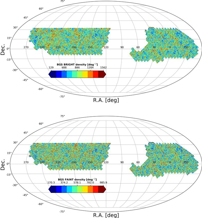
2 Omar A. Ruiz-Macias et al.
to carry out a number of wide-field surveys of galaxies and quasars surface density of galaxies and their clustering. A complementary
to map the large-scale structure of the Universe. These surveys will study by Kitanidis et al. (2020) examined the impact of imaging
probe the form of dark energy by allowing high precision measure- systematics on the selection and clustering of targets in the LRG,
ments of the baryon acoustic oscillation (BAO) scale and the growth ELG and QSO DESI surveys, using an earlier release of the Legacy
rate of structure using redshift-space distortions (RSD). The char- Surveys imaging data (Dey et al. 2019).
acterisation and definition of the target list for each DESI survey Here, we define and characterized the BGS target selection
is a critical step for efficient survey execution and to allow reliable based on the latest DECaLS release, DR8, which covers ∼ 2/3 of
measurements of galaxy clustering. Here we describe this process the full 14 000 deg2 of DESI footprint. The resulting catalogue is
for the DESI bright galaxy survey (hereafter BGS), a flux limited defined in Ruiz-Macias et al. (2020) and here we present the details
sample of around 10 million galaxies, using photometry from a new of that selection and associated analysis of the catalogue. This BGS
imaging survey, the Legacy Surveys2 (LS). catalogue was used by DESI in the commissioning stage of the
 DESI is a robotically-actuated, fibre-fed spectrograph that is early survey validation observations. It is planned that the final
capable of collecting 5 000 spectra simultaneously. BGS catalogue will be based on the next, DR9, Legacy Survey data
 The spectra cover the wavelength range 360 to 980 nm, with a release. This release will include better modelling of large galaxies
spectral resolution of = /Δ between 2 000 and 5 500, depending and the light in bright star haloes. More discussion of DR9 and
on the wavelength. DESI will be used to conduct a five-year survey planned subsequent characterization of the BGS selection can be
starting in 2020, with the aim of measuring redshifts over a solid found in Section 6.
angle of 14 000 deg2 . More than 30 million spectroscopic targets This paper is organised as follows: in Section 2 we describe
will be selected for four different tracer samples drawn from the the Legacy Surveys imaging data used to select our targets and
imaging data. These are (i) luminous red galaxies (LRGs) in the the secondary datasets used to tune the selection. In Sections 3
redshift range = 0.3 to = 1, (ii) emission line galaxies (ELGs) and 4 we define the spatial and photometric cuts used to select BGS
to = 1.7, (iii) quasars to higher redshifts (2.1 < < 3.5), and (iv) targets and to get rid of artifacts that might become problematic for
a magnitude-limited BGS out to ≈ 0.6 with a median redshift of DESI observations plus the removal of poor quality imaging data. In
 ≈ 0.2 which is the focus of this paper. Section 4 we define our star-galaxy classification using Gaia DR2.
 DESI observations are divided into two main programmes: the In Section 5 we compare the BGS catalogue with its overlap of the
Bright Time Survey (BTS) and the Dark Time Survey (DTS). The GAMA DR43 (Driver et al. 2012; Liske et al. 2015; Baldry et al.
BGS will be part of the BTS and is conducted when the Moon 2017) to assess the completeness and contamination of the BGS
is above the horizon and the sky is too bright to allow efficient and to quantify its expected redshift distribution. In Section 5.2 we
observation of fainter targets. The BTS excludes the few nights look at eight potential systematics that might be affecting our BGS
closest to full Moon and BGS always targets fields that are at least target selection and try to mitigate these effects with linear weights
40 − 50 deg away from the Moon. BGS alone will be ten times determined using the stellar density. Section 5.3 shows the clustering
larger than the SDSS-I and SDSS-II main galaxy samples (MGS) of our BGS selection before and after applying the weights and we
of 1 million bright galaxies that were observed over the time period compare it with SDSS and the MXXL lightcone catalogue (Smith
1999 − 2008 (Abazajian et al. 2003). et al. 2017). Finally, in Section 6, we summarize our results and
 The target sample for the BGS is intended to be a galaxy present our conclusions.
sample that is flux-limited in the -band. The magnitude limit is
determined by the total amount of bright observing time and the
exposure times required to achieve the desired redshift efficiency.
This target selection is, in essence, a deeper version of the target
selection for the SDSS MGS (Strauss et al. 2002).
 2 PHOTOMETRIC DATA SETS
 To make predictions for BGS target sample we make use of the
mock galaxy catalogue created from the Millennium-XXL (MXXL) During the BGS target selection process we make use of several
 -body simulation of Angulo et al. (2012) by Smith et al. (2017). catalogues. The main data set used is the Legacy Surveys DR8
This mock is tuned match the luminosity function, colour distribu- (hereafter LS DR8) imaging catalogue from which we select our
tion, and clustering properties of the SDSS MGS at low redshift, and targets. We also make use of secondary catalogues for masking
the evolution of these statistics to redshift ≈ 0.5 as measured from purposes, such as the Tycho-2 star catalogue (Høg et al. 2000), the
the GAMA survey (Driver et al. 2012; Liske et al. 2015; Baldry Gaia DR2 (Gaia Collaboration et al. 2016a), the Siena Galaxy Atlas
et al. 2017). - 2020 (SGA-2020) (Moustakas in prep.) and globular clusters from
 The DESI BGS is expected to have a target density of just the OpenNGC4 catalogue. We also use a combination of Gaia DR2
over 800 galaxies per square degree in a primary sample defined and LS photometry to perform star-galaxy separation.
by a faint -band magnitude limit of 19.5. Then, in a lower priority
sample, a secondary sample of ∼ 600 galaxies deg−2 defined by
the magnitude range 19.5 < < 20 (DESI Collaboration et al.
2016). From hereon in we will refer to these BGS samples as BGS
 3 This is an unreleased version of GAMA catalogue that the GAMA col-
BRIGHT and BGS FAINT respectively. A few per cent of galaxies in
the DESI BGS will be lost due to deblending errors, superposition laboration made available to us. It is essentially the same as GAMA DR3,
with bright stars, and other artifacts that typically affect imaging but with more redshifts.
 4 OpenNGC, https://github.com/mattiaverga/OpenNGC, is a
catalogues. Our aim is to provide a reliable input galaxy catalogue
 database containing positions and main data of NGC (New General Cat-
for the DESI BGS and to characterize its properties, such as the
 alogue) and IC (Index Catalogue) objects constructed by the GAVO data
 center team by merging data from NED, HyperLEDA, SIMBAD, and sev-
 eral databases available at HEASARC (https://heasarc.gsfc.nasa.
2 http://legacysurvey.org/ gov/).

 MNRAS 000, 1–22 (2021)

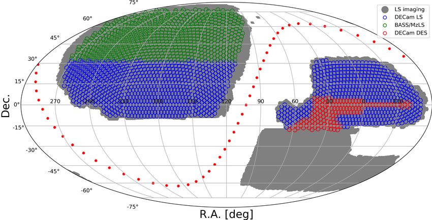
Target selection for the DESI BGS 3
2.1 Legacy Survey DR8 (DECam) in Tucson (NSF’s OIR Lab) through the NSF’s OIR Lab Community
 Pipeline8 (CP). The CP takes raw data as an input and provides de-
The Dark Energy Camera Legacy Survey (DECaLS), the Beijing-
 trended and calibrated data products such as instrumental calibration
Arizona Sky Survey (BASS), and the Mayall -band Legacy Survey
 (e.g. bias subtraction and flat fielding), astrometric calibration (e.g.
(MzLS) together constitute the DESI Legacy Imaging Survey (here-
 mapping the distortions and providing a world coordinate system,
after the Legacy Survey). The imaging Legacy Survey was created
 or WCS), photometric characterization (e.g. magnitude zero point
with the aim of attaining photometry with the necessary target den-
 calibration) and artifact identification, masking and/or removal (e.g.
sity, coverage and depth required for DESI. The SDSS MGS (Strauss
 removal of cross-talk and pupil ghosts, and identification and mask-
et al. 2002) and Pan-STARRS1 (Chambers et al. 2016) catalogues
 ing of cosmic rays).
are both too shallow to be used to reliably select the DESI survey
 The source catalogues for the Legacy Surveys are constructed
targets. The DES survey (The Dark Energy Survey Collaboration
 using the legacypipe9 software, which uses the TRACTOR10 (Lang
2005) does reach the target depth for DESI, but only covers 5000
 et al. 2016) code for pixel-level forward-modelling of astronomical
deg2 , mostly in the South Galactic Cap (SGC), with only ∼ 1130
 sources. This is a statistically rigorous approach to fitting the differ-
deg2 observable with DESI.
 ing point spread functions (PSF) and pixel sampling of these data,
 This work is based on the eighth release of the Legacy Survey
 which is particularly important as the optical data have a typical
project (LS DR8) which is the first release to integrate data from
 PSF width of ∼ 1 arcsec.
all of the individual components of the Legacy Surveys (BASS,
 The steps in the legacypipe processing are described in Dey
DECaLS and MzLS). However, this paper focuses only on DECaLS
 et al. (2019); we briefly summarize relevant parts here.
data.
 After initial source detection and defining the contiguous set of
 The DECaLS data in the LS DR8 data release comprises ob-
 pixels associated with each detection (termed a blob), legacypipe
servations from 9th August 2014 through 7th March 2019. DECam
 proceeds to fit these pixels with models of the surface brightness,
images come from the Dark Energy Camera (DECam Flaugher
 including a point-source and a variety of galaxy models. These fits
et al. 2015) at the 4-m Blanco telescope at the Cerro Tololo Inter-
 are performed on the individual optical images (in , and bands),
American Observatory. DECam has 62 2048 × 4096 pixel format
 taking into account the different PSF and sensitivity of each image,
250 m-thick LBNL CCDs arranged in a roughly hexagonal ∼ 3.2
 using TRACTOR.
deg2 field of view. The pixel scale is 0.262 arcsec/pix and the
 Besides the PSF model, TRACTOR fits four other light profile
camera has high sensitivity across a broad wavelength range of
 models to sources: a round exponential with a variable radius (re-
∼ 400 − 1000 nm. Since LS DR8 data goes beyond the intended
 ferred to as REX), an exponential profile (EXP), a de Vaucouleurs
DESI footprint5 of ∼ 14 000 deg2 , we are going to consider only
 profile(DEV), and a composite of DEV and EXP profiles (COMP).
data within the DESI footprint. This corresponds to ∼ 9 717 deg2
 The decision as to whether or not to retain an object in the catalogue
of DECaLS data of which ∼ 1 114 deg2 are covered by DECam
 and the choice of the model to best describe its light profile is treated
data coming from the DES (The Dark Energy Survey Collaboration
 as a penalized- 2 model selection problem.
2005). We essentially have two DECam data sets, i) DECam imag-
 This process results in object fluxes and colours that are con-
ing taken for the LS programme which we refer to as DECam LS
 sistently measured across the wide-area imaging surveys that form
and ii) the DECam data coming from the DES programme which
 the input into the DESI target selection. In general, TRACTOR
we refer to as DECam DES. DECam LS and DECam DES combine
 improves the target selection for all DESI surveys by allowing infor-
to form the DECaLS data set. Fig. 1 shows the sky map coverage of
 mation from low resolution and low signal-to-noise measurements
DECaLS imaging indicating the DECaLS imaging that lies within
 to be combined with those from high resolution and high signal-
the DESI footprint. DECaLS is the only survey that covers the entire
 to-noise data. The TRACTOR catalogues include source positions,
SGC (4 394 deg2 ) and the NGC (5 323 deg2 ) regions of the DESI
 fluxes, shape parameters, and morphological quantities that can be
survey at declination ≤ +32.375°.
 used to discriminate extended sources from point-sources, together
 In order to fulfil the target selection required for the different
 with errors on these quantities. The BGS is flux limited in the -
DESI surveys (BGS, LRGs, ELGs and QSOs), it was concluded
 band. However, since TRACTOR performs simultaneous fits in ,
that a three-band , and optical imaging programme, comple-
 and we also chose to impose quality cuts in the other bands as
mented by Wide-field Infrared Survey Explorer (WISE) W1 and W2
 well as those in the band when selecting the BGS targets.
photometry, would be sufficient. The minimal depth6 required is
 The main TRACTOR outputs required for the BGS are the total
 = 24.0, = 23.4 and = 22.5. DECam LS reaches these required
 fluxes11 corresponding to the best-fitting source model (i.e., PSF,
depths in total exposure times of 140, 100 and 200 sec in , , 
 REX, EXP, DEV or COMP) in all three bands ( , and ), the num-
respectively in nominal7 conditions, typically in a minimum of two
 ber of observations (NOBS) in the three bands, the predicted flux
visits per field.
 (in the -band only) within the aperture of a fibre which is around
 All data from the Legacy Surveys are first processed at the
 1.5 arcsec diameter (FIBERFLUX12 ) in 1 arcsec Gaussian seeing.
NSF’s National Optical-Infrared Astronomy Research Laboratory
 The Galactic extinction values are derived from the SFD98 maps
 (Schlegel et al. 1998) and are reported in linear units of transmission
 (MW_TRANSMISSION) in the , and bands, with a value of
5 Current LS DR8 imaging covers around ∼ 20 332 deg2 of which 15 174

deg2 corresponds to DECaLS.
6 The depths are defined as the optimal-extraction (forced-photometry) 8 https://www.noao.edu/noao/staff/fvaldes/CPDocPrelim/
depths for a galaxy near the limiting depth of DESI, where that galaxy is de- PL201_3.html
 9 https://github.com/legacysurvey/legacypipe
fined to be an exponential profile with a half-light radius of half = 0.45 arc-
sec. 10 https://github.com/dstndstn/tractor
7 Here ‘nominal’ is defined as photometric and clear skies with seeing 11 The fluxes output by TRACTOR are in units called NANOMAGGIES.

FWHM of 1.3 arcsec, airmass of 1.0, and sky brightness in , and of A flux of 1 NANOMAGGIE corresponds to an AB magnitude of 22.5.
22.04, 20.91 and 18.46 AB mag arcsec−2 , respectively. 12 The FIBERFLUX is in units of NANOMAGGIES

MNRAS 000, 1–22 (2021)

4 Omar A. Ruiz-Macias et al.

Figure 1. The sky map of the footprint of all the LS imaging used in DECaLS and in BASS and MzLS is shown in gray. The red and blue circles show the
DESI tiles that define the portion of DESI survey footprint that lies within DECaLS. The blue tiles are those for which the data comes from the DECam LS
imaging while the red tiles come from DECam DES imaging. The green tiles show the northern DESI footprint whose imaging data comes from the BASS
and MzLS surveys which are not the focus of this paper. The red dots show the locus of the Galactic plane.

unity representing a fully transparent region of the Milky Way and Table 1. The area, in square degrees, of DECaLS DR8 covered by at least
0 indicating a fully opaque region. The extinction coefficients for 1, 2 or 3 passes in each of the three filters ( ) individually (first three
the DECam filters were computed through an airmass of 1.3, for rows), and combined (i.e. at least 1, 2 or 3 passes in each of the 3 bands;
a source with a 7 000 K thermal spectrum (Schlafly & Finkbeiner bottom row). We have restricted our results to observations within the DESI
2011). The resulting coefficients are / ( − ) = 3.995, 3.214, footprint as shown in Fig. 1.
2.165, 1.592, 1.211, 1.064 in . These are then multiplied by Band/Number of Passes ≥1 ≥2 ≥3
the SFD98 ( − ) values at the coordinates of each object to de- -band 9 687 9 454 7 769
rive the , and MW_TRANSMISSION values. Finally, in each -band 9 686 9 422 7 569
band, there is a set of quality measures called FRACMASKED, -band 9 686 9 487 8 036
FRACFLUX and FRACIN that quantify the quality of the data in combined 9 669 9 257 6 870
each profile fit. We describe these in more detail in Section 4.4.
 The fluxes returned by TRACTOR can be transformed into AB
magnitudes as follows: 2.2.1 Tycho 2
 Bright stars can impinge upon the estimation of the photometric
 = 22.5 − 2.5 log10 (FLUX), (1) properties of nearby galaxies or may even lead to the generation
 = 22.5 − 2.5 log10 (FLUX/MW_TRANSMISSION),(2) of spurious sources. Hence, it is prudent to simply exclude or veto
 regions close to known bright stars to avoid such problems. Re-
where Eqn. (1) does not include the correction for Galactic extinc- gions near bright stars are masked out of the target catalogue using
tion, unlike Eqn. (2). The in Eqn. (1) stands for raw. the Tycho-2 catalogue (Høg et al. 2000). The Tycho-2 catalogue
 Table 1 shows the area covered by photometry in each of the contains positions, proper motions, and two-colour photometry for
three bands of DECaLS DR8 with 1, 2 or 3 passes. These values 2 539 913 of the brightest stars in the Milky Way.
are just for the data within the DESI footprint, as shown in Fig. 1.
This DECaLS footprint covers a total of 9 717 deg2 . Expressed in
percentages, 99.5 per cent of this area has at least one pass in all of 2.2.2 Gaia DR2
the three bands , 95.3 per cent has at least two passes and 70.7
per cent has at least three passes in all three bands. Gaia (Gaia Collaboration et al. 2016a) is a European Space Agency
 mission that was launched in 2013 with the aim of observing ≈ 1 per
 cent of all the stars in the Milky Way, measuring accurate positions
 for them along with their proper motions, radial velocities, and opti-
 cal spectrophotometry. The wavelength coverage of the astrometric
2.2 Secondary catalogues
 instrument, defined by the white-light photometric -band magni-
Here we list other catalogues that are used either to exclude regions tude, is 330 - 1050 nm (Carrasco et al. 2016). These photometric
of the sky in which the extraction of galactic sources is compro- data have a high signal-to-noise ratio and are particularly suitable
mised by the presence of other objects, or to perform star-galaxy for variability studies.
separation. Since the first release of Gaia data (Gaia Collaboration et al.

 MNRAS 000, 1–22 (2021)

Target selection for the DESI BGS 5
2016b), this survey has been widely used by the DESI LS (i.e. for the NSF’s OIR Lab CP tracks and TRACTOR reports in the LS
astrometric calibrations, proper motions, bright star masking) and is catalogue17
also ideal for constructing a star-galaxy separator for the BGS. There One way to avoid contamination of the catalogue with spurious
are 1.7 billion stars in the second Gaia data release (DR2)13 , over objects is to exclude regions around bright stars and galaxies. This
the whole sky to = 20.7, which is sufficiently deep to detect all can be done with a simple but effective circular mask for stars and
stars that might contaminate the BGS FAINT sample. We describe by using elliptical masks for galaxies. In Section 3.1 we set out
how we use a combination of Gaia and LS photometry to perform the geometrical masking functions we have applied around bright
star-galaxy separation in Section 4.1. stars, large galaxies and globular clusters to minimize the number of
 spurious targets in our BGS catalogue. In Section 3.2 we describe
 the masks applied to reduce the number of spurious targets due to
2.2.3 Globular clusters and planetary nebulae imaging artifacts such as bad pixels resulting from saturation and
 bleed trails.
Globular clusters and planetary nebulae are bright extended sources For subsequent analysis (e.g. estimating clustering statistics),
that can affect the identification of extragalactic sources in a similar it is very important to keep a record of the areas of the survey that
way to bright stars. In the LS, an area of sky around such ob- are removed by these masks. For this purpose we have made use
jects is excluded to minimize their impact on target selection. The of the randoms catalogue developed by the DESITARGET18 team.
OpenNGC catalogue14 is used to provide a list of such sources. The The randoms catalogue has a total density of 50 000 objects/deg2
extent and impact of masking around globular clusters and planetary divided into 10 subsets, each with density of 5 000 objects/deg2 .
nebulae is discussed in Section 3.1.3. Each random carries with it some of the DECam imaging infor-
 mation computed from the image pixel (in each band and expo-
 sure) in which it is located and supplementary information such as
2.2.4 The Siena Galaxy Atlas the dust extinction extracted from HEALPix19 maps (Zonca et al.
 2019). These imaging attributes include the number of observa-
Large galaxy images can be broken up by photometric pipelines,
 tions (NOBS_G, NOBS_R, NOBS_Z), galactic extinction (EBV),
which, for example, could mistake H II regions inside the galaxy for
 the bitwise mask for optical data (MASKBITS), etc20 .
individual extended sources. Also, spurious sources could be gen-
 In Fig. 2 we show a flow chart which summarizes the spatial
erated around the boundaries of large galaxies. The Siena Galaxy
 masking applied when constructing the BGS catalogue. The spatial
Atlas - 2020 (SGA-2020)15 is an ongoing project to select the
 masking is broken down into two classes: geometrical masking and
largest galaxies in the LS using optical data from the Hyper-
 pixel masking. The blue boxes of the flow chart report the survey
Leda catalogue16 (Makarov et al. 2014) and infrared data from
 area (in deg2 ) and mean target densities (in objects/deg2 ) after
the ALLWISE catalogue (Secrest et al. 2015). Currently the cat-
 successively applying each mask (gray hexagonal boxes). The red
alogue contains 535 292 galaxies that have an angular major axis
 boxes record the same information for the rejected area and objects.
(at the 25 mag/arcsec2 isophote) larger than 20 arcsec. The use
 The final BGS catalogue does not depend on the order in which
of the SGA-2020 in the spatial mask of the BGS is described in
 the masks are applied, but as some areas and targets are rejected by
Section 3.1.2.
 more than one mask the information in the red boxes depends on
 the ordering. For example, the area and number of objects shown
 as being rejected by the pixel masking excludes what would be
 rejected by this mask if the geometric masks had not been applied
3 SPATIAL MASKING
 first. Overall, for the DECaLS footprint of 9 717 deg2 , the spatial
Our main goal is to produce a reliable BGS input catalogue that masking removes 3.25 per cent of the area.
fulfils the DESI science requirements. If the target list contains
spurious objects, these will mistakenly be allocated fibres leading
to a reduction in the efficiency and completeness of the redshift 3.1 Geometrical masking
survey. Furthermore, spurious objects could imprint a systematic
effect in the measured clustering. 3.1.1 Bright star mask (BS)
 A step towards minimising the number of spurious objects is The bright star (BS) mask is based on the locations of stars from
to mask out regions of the sky around bright stars, since features Gaia DR2 (Gaia Collaboration et al. 2018) and the Tycho-2 (Høg
such as extended halos, ghosts, bleed trails and diffraction spikes et al. 2000) catalogue after correcting for epoch and proper motions.
around the stars can compromise the measurement of the photome- This mask consists of the union of circular exclusion regions around
try of neighbouring objects. Similarly we must remove areas around each star, where the radius of the exclusion region, estimated from
very large galaxies and globular clusters and planetary nebulae; an earlier stacking analysis, depends on the magnitude of the star in
such objects can also affect the photometric measurements of their the following way:
neighbours, leading to incorrect properties or spurious objects.
 Within the same framework, we have to propagate instrumental
effects such as saturated pixels, bad pixels, bleed trails, etc. that 17 In the LS DR8 catalogue information on whether or not the photometric
 parameters measured for an object have the possibility of being influenced
 by a bad pixel is flagged by the ALLMASK MASKBITS.
13 DR2 covers 22 months of observations and was released on 25 April 18 https://github.com/desihub/desitarget

2018. 19 http://healpix.sourceforge.net
14 https://github.com/mattiaverga/OpenNGC 20 For more information on the properties of randoms see:
15 https://github.com/moustakas/SGA http://legacysurvey.org/dr8/files/#random\protect\
16 http://leda.univ-lyon1.fr/ discretionary{\char\hyphenchar\font}{}{}catalogs

MNRAS 000, 1–22 (2021)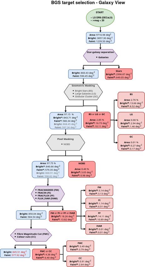

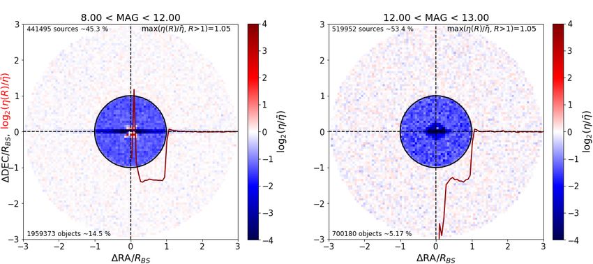
6 Omar A. Ruiz-Macias et al.
 These Tycho-2 stars represents only a 0.4% of total stars used for the
 BS masking. Then the magnitude, , used to compute the mask ra-
 dius in equation (3) is the Gaia -band magnitude for the Gaia stars
 and the Tycho-2 visual magnitude, mag_vt, for the retained Tycho-2
 stars. The overall median difference between the Tycho-2 and Gaia
 magnitude is 0.4 with Tycho-2 being fainter. This 0.4 magnitude
 difference translates into a median decrease in masking radius of
 50 arcsecs for Gaia stars with magnitude of 3 and a decrease of
 2 arcsecs for Gaia stars with magnitude of 13 from equation 3.
 Within BS ( ) TRACTOR forces all the sources it detects to be fit
 with the PSF profile to avoid artificially fitting diffraction spikes and
 stellar haloes as large extended sources. Thus any galaxies detected
 within BS will have their fluxes underestimated. Consequently to
 define a reliable galaxy catalogue we must veto all sources within
 BS of a bright star. In Fig. 2 we show that this Bright star mask
 covers 2.76 per cent of the initial footprint and rejects ∼195 po-
 tential BGS BRIGHT objects/deg2 and ∼31 potential BGS FAINT
 objects/deg2 when averaged over the full initial footprint. It should
 be noted that most of these objects are stars as star-galaxy separation
 has not been applied at this stage in the flow chart shown in Fig. 2.
 An alternative ordering of the flow chart with star-galaxy separation
 applied first is shown in Fig. A1. There we see that for galaxies the
 corresponding numbers are 13.7 galaxies/deg2 for BGS BRIGHT
 and 8.5 galaxies/deg2 for BGS FAINT.

 To determine if the bright star mask is adequate or whether the
 effects of stellar haloes causes a systematic error in the photometry
Figure 2. The flow chart shows the effects of the spatial masks that are of neighbouring galaxies that extends to larger radii, we plot in
applied as part of BGS target selection for the DECaLS DR8 data. The spatial Fig. 3 the average density of BGS galaxies in the vicinity of bright
masking is divided into two classes, one defined by the geometrical cuts stars prior to applying the bright star mask. If the photometry of
which exclude regions around bright sources (bright stars, large galaxies and galaxies has been compromised in any means, this can be seen in
globular clusters), and the other by pixel-based cuts which use information the galaxy number density to a fixed magnitude due to the strong
such as the number of observations (NOBS). The boxes in the flow chart dependence of galaxy number density on apparent magnitude. The
show the survey area (in deg2 ) and the target number density (per square term BGS galaxy refers to the BGS sample after applying the star-
deg) split into BGS BRIGHT and BGS FAINT after each mask is applied. galaxy separation and the spatial and photometric cuts down to the
The blue boxes give this information for the portion of the survey that is
 -band magnitude of 20, which will be covered in the subsequent
retained while the red boxes give this information for the areas removed.
 subsections of Section 3 and in Section 4. The stacks are made by
If more than one mask is combined at a single stage (as indicated within
the gray hexagonal boxes), then the dark-red boxes show the results for the expressing the angular separation, , of the BGS galaxies prior to
combination of these masks and the light-red boxes shows the results for apply the bright star mask from their nearest bright star in units of the
each individual mask. As some of the masks can overlap the numbers in the bright star masking radius BS , as given by Eqn. 3. In these rescaled
light-red boxes do not necessarily add up to those in the dark-red boxes. The coordinates, = / BS , galaxies within a radius of unity, shown by
target densities with the (∗ ) superscript are computed without correcting for the black circle, are within the BS masking zone. We show stacks
the area removed by the masking while those without the (∗ ) superscript for two magnitude bins defined by the -mag and visual magnitude
are corrected for the masked area. The gray hexagonal boxes describe the mag_vt for Gaia DR2 and Tycho-2 stars respectively, one with
different masks. Note that star-galaxy separation is not yet applied here and bright stars of magnitude between 8 to 12 and one fainter with
this is why we have a high target density in the blue boxes.
 magnitude between 12 to 13. The radial profile (red solid line) shows
 the variation in the target density, defined as Δ ( ) ≡ log2 ( ( )/ ) ¯
 where ( ) is the target density in an annulus at radius of width
 Δ ∼ 0.06, and ¯ is the mean target density evaluated over the
 BS ( ) = 39.3 × 2.5 (11− )/3 arcsec, > 2.9 (3) region 1.1 < < 3. This means that Δ ( ) = 0 corresponds to the
 = 471.6 arcsec, < 2.9. mean density, Δ ( ) ≥ 1 to an overdensity at least twice the mean
 density, and Δ ( ) < 0 to an underdensity. The large underdensity
Here is either Gaia -mag or Tycho-2 mag_vt with Gaia -mag at radius ≤ 1 is due to TRACTOR forcing all objects within this
being used when both are available. Stars fainter than = 13 have region to be fit by the PSF model. In Section 4.1 we will see how
no exclusion zone around them. stars and galaxies are defined for BGS target selection, which does
 The BS masking uses a total of 773 673 Gaia DR2 objects not depend on TRACTOR PSF designation, therefore, galaxies in
(82 objects/deg2 ) with Gaia -mag brighter than 13, while from the region < 1 are allowed. In the left panel of Fig. 3, we see a
Tycho-2, we have a total of 3 349 objects (∼ 0.36 objects/deg2 ) to spike of spurious galaxies for < 0.2. In contrast the right panel
a Tycho-2 visual magnitude brighter than mag_vt = 13. In order shows a strong deficit of galaxies at < 0.2. For > 1, the stacks
to avoid overlaps both catalogues have been matched after applying show uniform density close to mean, suggesting the star mask is
proper motions to bring Gaia objects to the same epoch as Tycho-2 working. There is a small bump just outside the masking radius
and keeping only the Tycho-2 objects that are not found in Gaia. where a ∼ 6 per cent excess is seen in both panels. This may need to

 MNRAS 000, 1–22 (2021)

Target selection for the DESI BGS 7

Figure 3. 2D histograms of the positions of BGS objects relative to their nearest Bright Star (BS) taken from the Gaia and Tycho-2 sources down to -mag
and visual magnitude mag_vt of 13 respectively. These stacks are performed in magnitude bins in the BS catalogue from magnitude 8 to 12 (left) and 12 to
13 (right). The stacks are made using angular separations rescaled to the masking radius function given in Eqn 3, which means that objects within a scaled
radius of 0 to 1 will be masked out by the BS veto while objects with = / BS > 1 will not (here 2 = (ΔRA2 cos(DEC) 2 + ΔDEC2 ). The colour scale
 ¯ within the shell 1.1 < / BS < 3. The density ratio is shown on a log2 scale where red
shows the ratio of the density per pixel ( ) to the mean density ( )
shows overdensities, blue corresponds to underdensities and white shows the mean density. The black solid circle shows extent of the BS exclusion zone. The
red solid line shows the radial density profile on the same scale as the colour distribution log2 ( ( )/ )
 ¯ where ( ) is the target density within the annulus
at radius of width Δ ∼ 0.06.

be revisited for accurate clustering studies, but is not large enough 3.1.3 Globular cluster mask (GC)
to be a concern for the efficiency of target selection.
 The globular cluster (GC) mask works in a similar way to the BS
 mask, by applying a circular exclusion zone around the GC. The
 masking radius is defined by the major axis attribute for the object
 in the OpenNGC catalogue.
 The GC mask has the smallest impact of the geometric masks,
 rejecting only 0.01 per cent of the initial area, accounting for densi-
 ties of 6.3 objects/deg2 in BGS BRIGHT and 2.5 objects/deg2 in
3.1.2 Large galaxies mask (LG) BGS FAINT. TRACTOR also force fits as PSFs everything within
 this mask.
Without special treatment, large galaxies in which spiral arms and
other structures such as H II regions are resolved would be artificially
fragmented by TRACTOR into multiple sources. To avoid this and 3.2 Pixel masking
to achieve more accurate photometry for large galaxies in the SGA-
2020 catalogue (see §2.2.4), TRACTOR is seeded with different Some of the effects that compromise the photometry on a pixel ba-
priors, and within an elliptical mask centred on the large galaxy sis and the model fitting include bad pixels, saturation, cosmic rays,
TRACTOR fits secondary detections using only the PSF model. bleed trails, transients. The NSF’s OIR Lab DECam CP identifies
This reduces the spurious fragmentation of large galaxy images, but these instrumental effects during its various calibrations21 (see Ta-
also means that genuine neighbouring galaxies within the masked ble 5 in Dey et al. (2019) for a list of the calibrations) and these
area have compromised photometry. The elliptical mask that is used are passed through TRACTOR and compiled in the ALLMASK
has the same position, 25 mag/arcsec2 isophotal major axis angular BITMASK22 . ALLMASK denotes a source blob that overlaps with
diameter, D25 , semi-minor to semi-major ratio, / and position any of the mentioned bad pixels in all of the overlapping images.
angle, as the ones used to define the large galaxies in the SGA- Besides the bad pixels which arise due to instrumental defects,
 √
2020 catalogue. Defining an effective masking radius of = , the BGS requires a complete sample in the three bands ( , and ).
where and are the semi-major and semi-minor axes of the We therefore impose a requirement that there is at least one obser-
elliptical mask, the median masking radius for the LG galaxies is vation in each of the bands through the NOBS parameter. NOBS
10.8 arcsecs. stands for Number of Observations, and is defined as the number of
 We apply these same masks to reject objects from the BGS images that contributes to the source detected central pixel in each of
catalogue but then we reinstate the large galaxies provided they are
not also masked by the bright star or globular cluster mask. The area 21 The document that lists all the calibrations and which includes details
covered by the combined LG mask amounts to only 0.08 per cent about the various maskings can be found at: https://www.noao.edu/
of the initial area and the number of objects removed amounts to noao/staff/fvaldes/CPDocPrelim/PL201_3.html
5.7 objects/deg2 BGS BRIGHT and 2.4 objects/deg2 BGS FAINT 22 Details of this BITMASK can be found here: http://www.

objects over the full initial area. legacysurvey.org/dr8/bitmasks/#allmask-x-anymask-x

MNRAS 000, 1–22 (2021)

8 Omar A. Ruiz-Macias et al.
the bands. Both ALLMASK and NOBS are pixel-based and hence
this information is also available in the random catalogue. However,
we find that virtually all of the area ( 97 per cent) (and hence vir-
tually all of the randoms) rejected by ALLMASK is also rejected
by using NOBS = 0 (in any band). In addition, ALLMASK rejects
a significant number of objects (196 objects/deg2 ) but with a small
associated area ( 0.01 per cent of the full area). Virtually all the ob-
jects rejected by ALLMASK and many others are already rejected
by the quality cuts in FRACMASKED, FRACIN and FRACFLUX
(in any band); these cuts will be reviewed in Section 4.
 In conclusion, there is little to be gained from using ALL-
MASK and we have therefore decided to use only NOBS as our
pixel level mask, shrinking the area by 0.4 per cent and reduc-
ing the target density by 7.7 objects/deg2 in BGS BRIGHT and 2
objects/deg2 in BGS FAINT.

4 PHOTOMETRIC SELECTION
Following the spatial masking described in the previous section, the
next step in the construction of the BGS target list is to incorpo-
rate information about photometric measurements into the selection
process. According to the science requirements of the BGS and the
mock BGS catalogues made by Smith et al. (2017), the survey is
expected to have a target density of 800 galaxies deg−2 to an -band
limit of 19.5. For the faint sample (19.5 < < 20), which is second
priority in BGS, a density of 600 galaxies deg−2 is expected.
 One of the major challenges for the BGS is the separation of
stars and galaxies. In Section 4.1 we describe how we compare high
angular resolution point source magnitudes from Gaia DR2 (Gaia
Collaboration et al. 2018) with total magnitudes from the best- Figure 4. Flow chart of the BGS target selection in the Legacy Surveys DR8
fitting light profile model selected by TRACTOR to distinguish based on photometric considerations. The photometric selection of BGS
point sources from extended sources. targets is divided into four stages; star-galaxy separation, fibre magnitude
 In Section 4.2 we describe how we reject spurious objects that cuts (FMC), colour cuts (CCs) and quality cuts (QCs). The photometric cut
have incongruous light profiles by comparing their total magnitudes flow chart is a continuation of the spatial cut flow chart (Fig. 2) and therefore
with the fibre magnitude that TRACTOR computes from the fitted we start from the area and object densities reported at the end of the spatial
profile assuming 1 arcsec Gaussian seeing and 1.5 arcsec fibre di- cut flow chart. We report densities for the bright and faint samples separately,
ameter. We place a cut in the fibre magnitude versus total magnitude showing in blue boxes the values for the sources remaining after each of the
 BGS cuts. The densities of the removed objects are shown in red/pink boxes.
plane that is motivated by the locus of confirmed galaxies from the
 The different cuts applied are shown in purple hexagonal boxes.
GAMA DR4 survey.
 Further posterior cuts which use photometry include removing
colour outliers in − and − (see § 4.3), and applying quality cuts artificial neural networks (Odewahn et al. 1992; Bertin & Arnouts
that indicate low accuracy in the flux measurement for an object (see 1996), support vector machines (Fadely et al. 2012) and decision
§ 4.4). The quality cuts make use of the quantities FRACMASKED, trees (Weir et al. 1995). TRACTOR uses a rigorous statistical ap-
FRACFLUX and FRACIN measured by TRACTOR for each object proach to determine the best fitting light profile model to each
in each of the three bands ( ). These are defined and discussed in object. In this way it classifies objects as either point sources (PSF)
§ 4.4. or extended sources (DEV, EXP, COMP or REX). However, this
 In Fig. 4 we show the second part of the BGS target selection pipeline is not infallible and it is inevitable with ground based seeing
flow chart. This flow chart focuses on the photometric selection cuts that some compact galaxies will be misclassified as being of PSF
and starts from where the previous flow chart (Fig. 2), showing the type rather than extended. As we want to avoid incompleteness that
spatial cuts, left off. The BGS catalogue, in the DECaLS subregion, depends on the variable seeing of the images we have instead made
ends up having a reduced area of 9 401 deg2 out of the initial 9 717 use of the space based high angular resolution Gaia photometry to
deg2 , and target densities of 846 objects/deg2 and 578 objects/deg2 distinguish point sources from extended sources. This is possible
for BGS BRIGHT and BGS FAINT respectively. for the BGS as virtually23 all stars brighter than the BGS magnitude
 limit of < 20 are bright enough to be detected by Gaia.
4.1 Star-galaxy separation The Gaia DR2 catalogue (Gaia Collaboration et al. 2018) that
 we use is primarily a catalogue of stars but has some galaxy and
The classification of images as star or galaxies is an old problem that quasar contamination as reported by Bailer-Jones et al. (2019). This
is of great importance when defining target catalogues for the ef- means we cannot simply classify all of the BGS objects that are
ficient use of multi-object spectrographs. Sophisticated techniques
are employed which include algorithms using machine learning
methods applied to both colour and morphological information e.g. 23 Gaia DR2 is complete between 12 < -mag< 17.

 MNRAS 000, 1–22 (2021)

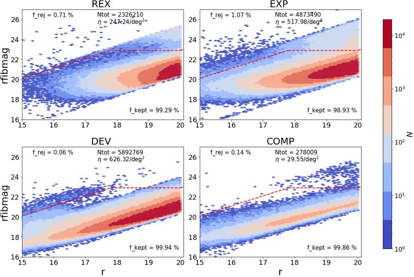
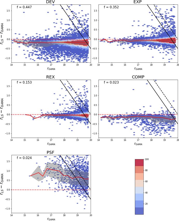
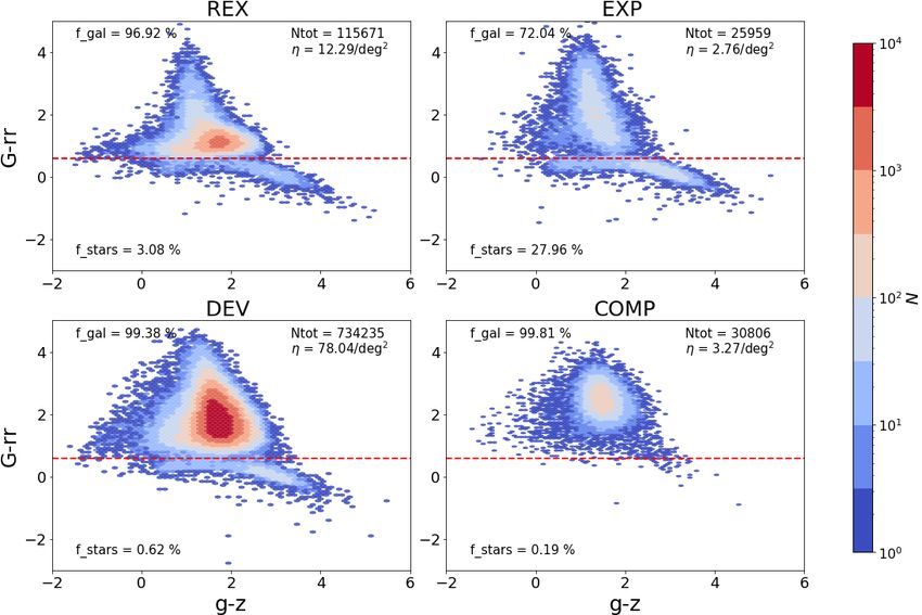
Target selection for the DESI BGS 9

Figure 5. Separately for objects classified by TRACTOR as type REX, EXP, DEV COMP and PSF we show the difference between the Gaia (PSF) magnitude
 and total non-dust corrected r-band model magnitude measured by TRACTOR, versus TRACTOR extinction corrected − colour. All the objects
plotted have passed the geometrical and pixel cuts detailed in Fig. 2, and all but the star-galaxy classification cut of the photometric-based cuts detailed in
Fig. 4. The plots show objects that have been cross-matched between LS DR8 objects and Gaia DR2. Each panel shows a different morphological class, as
labelled, according to the best-fitting light profile assigned by TRACTOR. The red-dashed line indicates our adopted division at − = 0.6 with stars below
and galaxies above the line. The colour in the plots shows the number counts of objects in an hexagonal cell, ranging from 1 to 10 000, except for the case of
PSF-type objects, in which case the colour scale covers the range from 1 to 1 million as indicated in the colour bars. We display the fraction of galaxies and
stars according to this classification at the top-left corner and bottom-left corner respectively. The total number of objects ( tot ) in each plot and the target
density ( ) this represents is displayed in the top-right corner.

Figure 6. BGS galaxies in the -band total magnitude (x-axis) versus -band fibre magnitude (y-axis) plane in the LS DR8. The results are divided into the five
different TRACTOR best-fitting light profile models, as labelled at the top of each panel. The colour bar shows the number counts of objects in an hexagonal
cell covering the range from 1 to 20 000 for four of the light profile models with the exception of PSF-type galaxies, in which case the scale covers 1 to 10 000.
The red-dashed line shows the fibre magnitude cut (FMC): we reject every object that is above this threshold. The numbers shown in top-left and bottom-right
corners give the fraction of galaxies rejected and kept, respectively, while the number in the top-right corner shows the total number of galaxies ( ) and
the corresponding target density ( ).

MNRAS 000, 1–22 (2021)

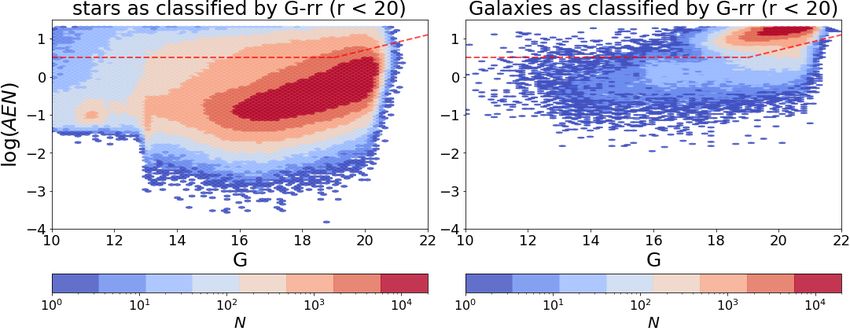
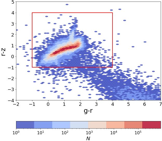
10 Omar A. Ruiz-Macias et al.
in Gaia as stars. However, by comparing TRACTOR magnitude The BGS target selection has the expected surface density after
measurements with the higher spatial resolution magnitude mea- applying the star-galaxy separation. From the spatial cut flow chart
surements from Gaia we can determine which objects have ex- in Fig. 4, we find a bright target density of 868.91 objects/deg2
tended light profiles. The Gaia magnitudes are computed assuming and a faint target density of 598.82 objects/deg2 . Rejected Gaia
all objects are point sources. This results in accurate magnitudes stars have a target density of 2 804.01 objects/deg2 bright stars and
for stars but magnitudes that are systematically fainter than the as- 622.80 objects/deg2 faint stars.
sociated total magnitudes for sources that are extended compared
to the ∼ 0.4 arcsec PSF achieved by Gaia. In contrast, the model
magnitudes computed by TRACTOR should capture more fully the 4.2 Fibre magnitude cut
total magnitude of the object. Consequently, if Gaia and TRACTOR In order to reduce the number of image artefacts and fragments
magnitudes were measured in the same band, we would expect them of ‘shredded’ galaxies that would otherwise be classified as BGS
to agree for point sources but for the TRACTOR magnitude to be targets we apply a cut on the fibre magnitude that is defined as a
brighter than the Gaia magnitude for extended sources. We would function of -band magnitude as follows:
even expect this to be true for extended objects that TRACTOR mis- (
classifies as PSF since the wide, ground-based PSF of TRACTOR 22.9 + ( − 17.8) for < 17.8
 rfibmag < (4)
would capture more of the total flux than the narrow PSF of Gaia. 22.9 for 17.8 < < 20
The complication is that the Gaia band is a much wider filter
than the DESI band, but as we shall see, the colour dependence is where rfibmag is the magnitude of the predicted -band fibre flux
weak. and is the total -band magnitude, both extinction corrected. The
 Based on these considerations we define TRACTOR objects location of this cut was guided by inspecting postage stamp images
with < 20 as being galaxies if either of the following two condi- of a selection of the objects with the faintest fibre magnitudes with
tions is met: the aim of rejecting objects that appear to be artefacts while retaining
 nearly all of the genuine galaxies. In addition, at the bright end our
 • The object is not in the Gaia catalogue. threshold was guided by the location of spectroscopically confirmed
 • The object is in the Gaia catalogue but has − > 0.6. GAMA galaxies, as discussed further in Section 5.1. Fig. 6 shows
 the distribution of the BGS objects in the rfibmag vs. rmag plane,
In the above, the -band is the photometric Gaia magnitude and
 with a separate panel for the different TRACTOR classes, and a
 is the raw -band magnitude from the LS DR8 without applying
 red-dashed line indicating the location of the fibre magnitude cut
a correction for Galactic extinction. This choice is made because
 (hereafter FMC). In the first four panels we can see that the galaxy
the Gaia magnitude is not corrected for Galactic extinction. The
 locus has a tight core and, in general, is well below the FMC. The
discussion above explains that and magnitudes are measured
 FMC removes 1.2 per cent of the objects classified as EXP and even
in different effective apertures and so the quantity − should be
 smaller fractions of the other light profile classes.
thought of as a measure of how spatially extended an object is and
 All BGS objects in the PSF class lie on a stellar locus. Whether
not its colour. The first criterion above is satisfied by most (93 per
 all these objects are stars or whether this is an artefact of TRACTOR
cent) of the BGS objects. It leaves very little stellar contamination
 only fitting the PSF model to Gaia sources with low astrometric
in the BGS, as essentially any star brighter than = 20 is bright
 excess noise (AEN) is revisited in Section 5.1, where we compare
enough to be detected and catalogued by Gaia. The second criterion
 our classification with that of the GAMA DR4 survey. The stellar
is required to keep the BGS completeness high by not rejecting
 locus is also visible in the other photometric classes indicating there
galaxies that are in the Gaia catalogue.
 is some stellar contamination in our sample, but it is at a very low
 In Fig. 5 we show the − versus − plane for objects in Gaia
 level.
DR2 that are matched with objects in the LS DR8. The panels show
 In summary the adopted FMC rejects a further 23.17
different objects as classified by the TRACTOR model fits (i.e.,
 objects/deg2 of which 11.72 are in BGS BRIGHT and 11.45 are
PSF, COMP, DEV, EXP, REX). The cross-matched objects have
 in BGS FAINT from the objects that have passed the previous cuts
been subject to all the BGS cuts (i.e. both spatial and photometric)
 which include the rejection of stars by our star-galaxy classifier.
with the exception of the star-galaxy separation itself. For objects
classified by TRACTOR as PSF-type, we can see the stellar locus
around − = 0 with a weak colour dependence. For the extended 4.3 Colour cuts
sources (i.e., COMP, DEV, EXP, REX), we see part of the galaxy
locus24 in the upper part of the plot, just above − = 0. An efficient way of rejecting further spurious targets from the BGS
 From Fig. 5 we can see that the assignment of the best fitting is to reject objects with bizarre colours. The limits we impose to
TRACTOR model supports our Gaia classification using − > reject outliers are:
0.6, but we can still see some remnants of the stellar locus for objects −1 < − 

Target selection for the DESI BGS 11

 Table 2. The BGS target densities for each of the TRACTOR best-fitting
 photometric models. The first column labels the photometric model. The
 next three columns list the surface density of objects per deg2 for the BGS
 BRIGHT and BGS FAINT samples separately and their combined sum. The
 area covered by the DECaLS portion of the BGS is 9, 401 deg2 .

 Model bright faint overall
 [deg−2 ] [deg−2 ] [deg−2 ]
 DEV 427 202 629
 EXP 284 230 514
 REX 104 141 246
 COMP 27 3 31
 PSF 3 2 5
 Total 846 578 1423

 (QCs):
 FRACMASKED_i < 0.4,
 FRACIN_i > 0.3,
 FRACFLUX_i < 5, where = , or , (6)
 based on visual inspection of postage stamp images.
Figure 7. Colour-colour distribution showing − vs. − for BGS As mentioned in Section 3.2, we find that the objects flagged by
objects without applying the CCs. The colour bar shows the number counts the TRACTOR quantity ALLMASK are essentially a subset of the
of objects in an hexagonal cell covering the range from 1 to 800 000. The
 objects that are rejected by applying the quality cuts listed in Eqn. 6.
solid red box shows CCs defined in Equation 5. Sources outside of this box
 While cutting on ALLMASK would have the advantage that it could
are excluded from the BGS.
 also be applied to the randoms, we find that it is important to apply
 the QCs to remove spurious objects that are missed by the other cuts.
 For instance, some spurious objects that are outliers in either the
more than a few objects/deg2 as we shall see in Section 5.1. The fibermag vs. mag plane or in the colour-colour space that just pass
colour cuts (CCs) we apply reject an additional 6.7 objects/deg2 , the FMC and CCs are removed by considering FRACMASKED or
with 2.66 in BGS BRIGHT and 4.04 in BGS FAINT. FRACIN.
 As shown in the flow chart, Fig. 4, the QCs reject an ad-
 ditional 14.11 objects/deg2 of which ∼ 60 per cent are re-
 moved by FRACFLUX, ∼ 45 per cent by FRACMASKED and
4.4 Quality cuts
 ∼ 7 per cent due to FRACIN. The overlap between the FRAC-
Each object in the TRACTOR catalogue has three measures of the MASKED, FRACIN and FRACFLUX cuts is minimal, with only
quality of its photometry recorded in each of the three bands ( ). 1.05 objects/deg2 for objects with < 19.5, and in round 0.15
These are: objects/deg2 for objects with 19.5 < < 20 being rejected by more
 than one of the cuts. Separately for BGS BRIGHT and BGS FAINT,
 • FRACKMASK (FM): The profile-weighted fraction of pixels we show the target density of objects rejected by these cuts after ap-
masked in all observations of the object in a particular band. This plying all the previous cuts. The largest overlap between these cuts
quantity lies in the range [0, 1]. High values indicate that most of is between FRACMASKED and FRACFLUX for BGS BRIGHT,
the flux of the fitted model lies in pixels for which there is no data but even here it amounts to less than 1 object/deg2 . For BGS FAINT
due to masking and so the measurement is unreliable. this overlap is small, 0.11 object/deg2 , and there is no overlap with
 • FRACIN (FI): The fraction of the model flux that lies within FRACIN.
the set of contiguous pixels (termed a ‘blob’) to which the model
was fitted. FRACIN is close to unity for most real sources. Low In Appendix A we present another version of the selection
values indicate that most of the model flux is an extrapolation of the cut flow chart in which the cuts are applied in a different order.
model into regions in which no data was available to constrain it. There we give a galaxy view of the target selection by first applying
 • FRACFLUX (FF): The profile-weighted fraction of the flux the star-galaxy classification so that all the subsequent cuts apply
from other sources divided by the total flux of the object in question. only to galaxies. The final selected sample which comprises of
FRACFLUX is zero for isolated objects but can become large for 845.5 galaxies/deg2 in BGS BRIGHT and 577.9 galaxies/deg2 in
faint objects detected in the wings of brighter objects that are nearby. BGS FAINT, is exactly the same, as the order of the cuts does not
 matter. The objects rejected by each filter, however, does change as
 Once the other cuts have been applied, in particular, the cut on many objects are rejected by more than one filter. To illustrate this
NOBS and the BS mask, the distribution of each of these quantities point we have also swapped the order of the FMC and QCs cuts so
is tightly peaked around the favoured values of FRACMASKED one can see how these influence one another.
≈ 0, FRACIN ≈ 1 and FRACFLUX ≈ 0. However, each quantity
has a distribution with a fairly featureless tail that extends out to less
desirable values. There are also clear correlations between the three
 5 CATALOGUE PROPERTIES
quantities for a given photometric band and in some cases between
photometric bands. The choice of the best set of thresholds to reject The final BGS catalogue in the DECam region in the South Galactic
outliers is not trivial. We have adopted the following quality cuts Cap (SGC) covers the declination range −17 . DEC . 32 degrees,

MNRAS 000, 1–22 (2021)