Lineage: Visualizing Multivariate Clinical Data in Genealogy Graphs - bioRxiv
←
→
Page content transcription
If your browser does not render page correctly, please read the page content below
bioRxiv preprint first posted online Apr. 19, 2017; doi: http://dx.doi.org/10.1101/128579. The copyright holder for this preprint
    (which was not peer-reviewed) is the author/funder, who has granted bioRxiv a license to display the preprint in perpetuity.
                                   It is made available under a CC-BY-NC 4.0 International license.

Lineage: Visualizing Multivariate Clinical Data in Genealogy Graphs
                                  Carolina Nobre, Nils Gehlenborg, Hilary Coon, and Alexander Lex

        Fig. 1. Lineage visualizing the genealogy of a family with an increased number of suicides. The genealogy view shows the family
        relationships in a linear tree layout, where each node corresponds to a row in the associated table. Suicide cases are highlighted in
        blue, a glyph next to the nodes indicates whether individuals were diagnosed with depression. Some branches are aggregated. The
        table shows detailed attributes about individuals, or, when branches are aggregated, for groups of individuals.

        Abstract— The majority of diseases that are a significant challenge for public and individual heath are caused by a combination of
        hereditary and environmental factors. In this paper, we introduce Lineage, a novel visual analysis tool, designed to support domain
        experts that study such multifactorial diseases in the context of genealogies. Incorporating familial relationships between cases can
        provide insights into shared genomic variants that could be implicated in diseases, but also into shared environmental exposures. We
        introduce a data and task abstraction and argue that the problem of analyzing such diseases based on genealogical, clinical, and
        genetic data can be mapped to a multivariate graph visualization problem. Our main contribution is a novel visual representation for
        tree-like, multivariate graphs, which we apply to genealogies and clinical data about the individuals in these families. We introduce
        data-driven aggregation methods to scale to multiple families with hundreds of members across several generations. By designing
        the genealogy graph layout to align with a tabular view that displays clinical data for each family member, we are able to incorporate
        extensive, multivariate attributes in the analysis of the genealogy without cluttering the graph. We also discuss how the principles of our
        methodology can be generalized to other scenarios. We validate our designs using an illustrative example based on real-world data,
        and report of feedback from domain experts.
        Index Terms—Multivariate networks, biology visualization, genealogies, hereditary genetics, multifactorial diseases.

1     I NTRODUCTION                                                            hereditary diseases. Geneticists, on the other hand, have long used
Studying ancestry and familial relationships, i.e., genealogies, is both       genealogical graphs to study how a genetic disease manifests itself in
a past-time enjoyed by amateurs and a research area for profession-            families. They use drawing conventions and standardized symbols to
als [35]. It is hence not surprising that there are a wealth of tools to       show both, the family structure and the phenotype, i.e., the observ-
record and visualize genealogies. Yet, most of these tools focus on            able characteristics of an individual [7, 6]. These charts can provide
analyzing family structures for historical purposes and only few target        insights about the heritability and segregation patterns of genetic dis-
a clinical use case of analyzing genealogies in the context of complex,        eases. In their current form, however, they are predominantly useful for
                                                                               Mendelian diseases, or genetic diseases caused by a small number of
                                                                               mutations. Complex diseases such as cancer, autism, diabetes, obesity,
• Carolina Nobre and Alexander Lex are with the University of Utah. E-mail:    and psychiatric conditions such as depression or suicide are known to
  {cnobre, alex}@sci.utah.edu.                                                 have hereditary components that are regulated by a multitude of genes,
• Hilary Coon is with the University of Utah. E-Mail: hilary.coon@utah.edu     each having a modest effect on risk, and also to depend strongly on
• Nils Gehlenborg is with Harvard Medical School. E-mail:                      environmental conditions and chance. When studying these conditions
  nils@hms.harvard.edu.                                                        in a population, it is imperative to simultaneously consider genetic
                                                                               similarities, shared characteristics of the phenotype, and environmental
                                                                               conditions. Also, for these polygenic conditions one needs to consider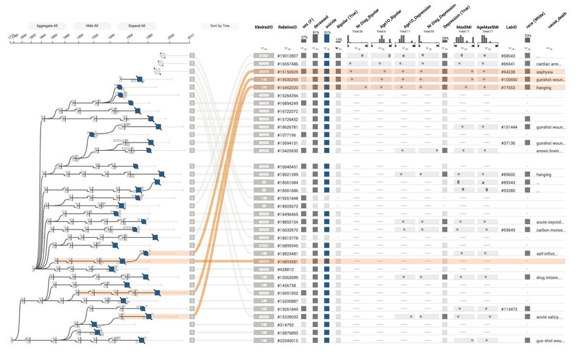
bioRxiv preprint first posted online Apr. 19, 2017; doi: http://dx.doi.org/10.1101/128579. The copyright holder for this preprint
     (which was not peer-reviewed) is the author/funder, who has granted bioRxiv a license to display the preprint in perpetuity.
                                    It is made available under a CC-BY-NC 4.0 International license.

significantly larger populations to reason about hereditary relationships                                                                Founder
and pursue discovery of genetic risk mutations.
    Current medical or historical genealogy1 visualization tools are ill
equipped to help researchers in finding patterns in these large, highly
multivariate graphs of families and their rich medical histories. In this
paper, we present a novel genealogy visualization tool that we have
developed in collaboration with psychiatrists and geneticists studying
the genetic underpinnings and the environmental factors of suicide and                          (a)                                 (b)
autism. We use data from the Utah Population database2 , a uniquely
                                                                                Fig. 2. Two genealogies using standardized symbols focusing on different
rich resource for population based analysis of hereditary diseases.             aspects of the family structure. Females are shown as circles, males as
    We contribute a novel technique to visualize large, tree-like graphs        squares. Individuals with a phenotype of interest are filled-in in black.
(rooted, directed graphs that have some cycles but are predominantly            (a) A genealogy showing the family of the female in black, including
in tree form) associated with rich numerical, categorical and textual           siblings, parents, uncles/aunts, and grandparents. (b) A genealogy
attributes. Our approach leverages the tree-like structure of the graphs        based on a founder, tracing down generations to include the families of
to produce a linearized layout which enables the direct association of          individuals with a phenotype of interest (black).
the nodes with rich attributes in a tightly integrated tabular visualization.
We address the issue of scalability by introducing novel forms of degree-       genealogy includes her two siblings and traces her family tree up for two
of-interest based aggregation that preserve the structure of the graph,         generations to include their parents, uncles and aunts, and grandparents.
and if desired also provide an overview of the attributes of aggregated             In contrast, our collaborators are interested in understanding genetic
individuals. While we demonstrate our technique in the context of               relationships between individuals afflicted with a condition and hence
genealogical data, we argue that it can equally be applied to other             care about individuals who share genetic variants. They select families
multivariate trees or tree-like graphs.                                         for study that have a statistically increased rate of a condition. These
    We also contribute a detailed characterization of the domain prob-          family trees are constructed by tracing cases back to a “founder”, as
lems and of the domain data as they are encountered when analyzing              illustrated in Figure 2(b). The underlying hypothesis is that the founder
large, clinical genealogies and a set of task and data abstractions derived     has genetic risk variants which they passed on to their descendants.
from these characterizations. Finally, we contribute the open source Lin-       Within the genealogy, the likelihood of genetic homogeneity is in-
eage visualization tool (http://lineage.caleydoapps.org),                       creased, and is more easily detected through the repeated occurrence of
shown in Figure 1, which implements the technique; and describe mul-            the genetic risk variant in the familial cases. Note that this genealogy
tiple design decisions tailored towards genealogical data visualization.        only contains individuals that are descendants of one founder and their
    Lineage is in the process of being adopted by our collaborators, and        spouse, with the exception of spouses of descendants. Also, the dataset
has undergone iterative design refinements. We have also demonstrated           only contains individuals with direct links to a case; i.e., siblings, de-
it to other research groups working with genealogical and genetic data          scendants, and direct ancestors are included, whereas, for example,
and have encountered overwhelming enthusiasm. We validate this work             uncles/aunts and cousins are not.
in an illustrative usage scenario and through qualitative user feedback             The dataset our collaborators have compiled contains about 19,000
from domain experts.                                                            suicide cases, including the 4,017 recent cases with detailed data,
                                                                                backed by family structures made up of 118,000 individuals from
2 D OMAIN BACKGROUND AND DATA                                                   551 families. Suicide is frequently associated with psychiatric co-
Our collaborators study the genetic underpinnings and the environ-              morbidities, i.e., co-occurring chronic conditions, such as depression,
mental factors influencing psychiatric conditions, such as autism and           bipolar disorder, substance abuse, PTSD or schizophrenia [46]. Also,
suicide, using detailed genealogical, clinical, and genetic data. In this       non-psychiatric conditions such as asthma [24] may play a role in some
paper, we will focus on suicide, yet our methods are easily transferable        cases. Environmental factors, such as socioeconomic status, pollution,
to other complex, multifactorial conditions and diseases. Suicide is a          and seasonality are also known to be factors in suicide [2]. To capture
high impact application, as it is one of the leading causes of life-years       this information, our datasets includes demographic variables such
lost [52], and the 10th most common cause of death in the United                as gender, race, age at death, method of death, family demographics
States [37]. Suicide is believed to be caused by a complex combination          (marriage, divorce, number of siblings/children), and place of residence
of risk factors, including environmental stressors, but also genetic vul-       at the time of death. It includes records of other diagnoses captured as
nerability. Aggregated data across multiple large studies has produced          codes from the International Classification of Diseases (ICD) systems,
heritability estimates of completed suicide of 45% [41, 33]. Genetic            the frequency with which these diagnoses were made, and the time of
risk factors for suicide are complex and can be classified into multi-          the first diagnosis.
ple subtypes. These subtypes often are characterized by co-occurring                To summarize, we have many graphs, each describing a family, with
psychiatric conditions (comorbidities), and/or combined risk of psy-            individuals as nodes and family relationships as edges. Since the graphs
chiatric diagnosis. For example, genetic risk for schizophrenia is also         are constructed by tracing ancestry to a founder, they are predominantly
associated with risk for suicide [46].                                          tree-like, but do include cycles, for example, when two cousins have
   Our collaborators have compiled a unique dataset of suicide cases,           offspring. In addition, we have attributes on the individuals/nodes in the
including DNA and clinical profiles on 4,017 cases. These cases are             graphs of various data types, including numerical, categorical, temporal,
linked to the Utah Population Database (UPDB), which provides ge-               geographic, and textual data. These attributes are often sparse, as only
nealogical data. Genealogies describe the familial relationships of             about 10% of individuals in the dataset have committed suicide, and our
individuals across multiple generations.                                        detailed records extend to only about 2% (4,017) of individuals across
   Figure 2 shows two genealogies using the standardized drawing                all families. These detailed records capture about 3,000 dimensions that
conventions [7, 6]. Females are drawn as circles, males as squares.             contain demographic information and information about the manner of
Couples are connected by an edge, children connect to this edge using           death, but predominantly contain comorbidities in the form of disease
orthogonally routed links. The vertical position of nodes is given by           codes, time of the diagnosis, and the frequency of the diagnosis. These
their generation. A phenotype of interest is marked by a filled-in node.        dimensions are themselves often sparse, as, among other reasons, a
   When studying family relationships, a common approach is to draw             colloquial diagnosis such as “depression” can be recorded using one of
family trees considering the ancestry of an individual. Figure 2(a),            about 30 ICD codes.
for example, shows the family of the women marked in black. The
   1 The                                                                        3   D OMAIN G OALS AND TASKS
          terms genealogy and pedigree can be used interchangeably in this
context. However, for simplicity, we will always use genealogy.                 This project is rooted in a collaboration with faculty, clinicians, analysts,
   2 https://healthcare.utah.edu/huntsmancancerinstitute/research/updb/         and graduate students in the Department of Psychiatry at the University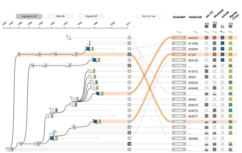
bioRxiv preprint first posted online Apr. 19, 2017; doi: http://dx.doi.org/10.1101/128579. The copyright holder for this preprint
  (which was not peer-reviewed) is the author/funder, who has granted bioRxiv a license to display the preprint in perpetuity.
                                 It is made available under a CC-BY-NC 4.0 International license.

of Utah. In total, six domain experts were involved in the process. We            branches of a single family. Judging how common a phenotype is
loosely followed the design study methodology by Sedlmair et al. [43].            in a family or a part of the family is helpful in identifying subsets
Our “discover” phase consisted of multiple meetings with individual               of interest for further study.
collaborators and with the whole group as a team, studying the domain
                                                                              T5 Compare families. Once an interesting observation has been
literature and the tools they currently use. We also ran a creativity
                                                                                 made in one family, our collaborators want to be able to inves-
workshop, specifically the “wishful thinking” component described by
                                                                                 tigate whether similar cases also appear in other families. For
Goodwin et al. [19], involving all of the collaborators. In the workshop,
                                                                                 example, when an association of asthma with suicide is discov-
we asked participants to think about the analysis of suicide data and
                                                                                 ered, it is important to know whether this is isolated in one family,
then discuss in small groups and take notes on post-its about what it is         or occurs in multiple families and/or individuals.
they would like to know, see, and do. This idea generation phase was
followed by a phase where the teams had to prioritize their insights,         T6 Quality control. While not an analysis task per-se, our collabo-
and then finally give the whole team an overview of their key ideas. We          rators also need to judge the quality of the data and report errors
recorded the workshop, and transcribed both the audio and the post-its.          back to the central database. A common data error we have seen,
We then coded the artifacts and three themes emerged: they described             for example, are disconnected components or detached nodes,
details about the data, the factors involved in suicide, and the analysis        which are caused by missing information about an individual’s
tasks. The insights about the data and the factors involved in suicide           mother and/or father.
are described in the previous section.                                         Most of these domain tasks rely both on studying the topology of the
    The overarching goal of our collaborators is to gain a better un-       network, i.e., the family relationships, and on investigating the attributes
derstanding of the determining or associated factors of suicide. They       associated with the individuals. For example, the “compare cases” task
classify these into comorbidities, demographic, genetic, and environ-       (T3) relies on both, the graph and the attributes to, for example, reject
mental factors. Specifically, they are interested in identifying and        an outlier in an otherwise well-defined phenotype within a family, if
defining detailed phenotypes associated with suicide and the degree to      that outlier is only distantly related to other cases.
which these phenotypes are familial. By finding people that are similar
to each other in a relevant way, our collaborators hope to reason about     4 R ELATED W ORK
genetic homogeneity, i.e., share genetic factors contributing to suicide.   We focus our discussion of previous work on specialized genealogy
They currently rely only on familial structure as a proxy for genetic       visualization tools and on multivariate network visualization, as ge-
homogeneity. However, they recognize that this is limited both as too       nealogies are highly multivariate graphs. With regards to multivariate
broad — it is possible that they should only consider a part of a family    network visualization approaches, we also restrict our discussion to
— and as too narrow — people outside a family that have a similar           explicit layouts (i.e., node link layouts), as implicit layouts (such as
phenotype could also have a similar genotype. Robust and detailed           SunBursts and treemaps) are ill suited to visualize attributes at all levels
phenotypes are of course also interesting by themselves, as they, for       of the hierarchy; and matrices are not an ideal choice for genealogies as
example, can be used as part of a risk assessment in a clinical context.    (a) the nodes are only sparsely connected, hence wasting a lot of space,
    It is important to note that the contextual knowledge of a researcher   and (b) matrices are ill suited for path tracing, which is a common task
is immensely beneficial to the task of classifying a phenotype. For         of our collaborators.
example, a diagnosis of depression is weighted differently if it is diag-
nosed dozens of times and was first diagnosed early in a patient’s life.    4.1 Multivariate Networks
Similarly, a suicide case at a young age in a rural community is unlikely   A multivariate network is a graph where the nodes and/or the edges
to have a detailed medical history. Hence, such a case could potentially    are associated with potentially rich attributes [25]. Many graph visual-
be similar to others, even if certain phenotypes are not recorded, if       ization techniques are optimized for either topology or attribute based
other factors, such as a close familial relationship indicate it.           tasks [49], yet in many applications topology and attributes have to
    We identified the following domain tasks as the most important          be judged in concert [39]. When analyzing genealogies, for example,
aspects in the workflows of our collaborators:                              our collaborators want to understand how two people with a similar
                                                                            phenotype are related, requiring them to first identify the phenotypes
 T1 Select families of interest. The analysts want to select a family       using the attributes, and then judge their relatedness using the topology
    either by browsing, or by selecting a specific family based on prior    of the genealogy.
    knowledge, or in a data driven way. An example of data-driven               Partl et al. [39] classify four basic approaches to visualize multi-
    selection of families is to find families with high rates of suicide,   variate networks for explicit graph layouts: (1) on-node mapping, i.e.,
    or to find families with individuals where suicide co-occurs with       visualizing the attributes by changing a visual channel of the node mark
    bipolar disorder.                                                       or by embedding a small visualization in the node; (2) small multiples,
 T2 Analyze individual case. Our collaborators need to investigate          i.e., showing the same graph multiple times and visualizing a different
    the context of a case. For example, a potential genetic component       attribute on top of each of the small networks, (3) separate, linked views
    contributing to suicide is judged differently if the person had         for the graph and the attributes, and (4) adapting the graph layout to
    many psychiatric comorbidities and committed suicide at a young         better fit the needs of attribute visualization.
    age, compared to a late-life suicide of a person with a terminal            These approaches have different strengths and weaknesses with
    disease.                                                                respect to the tasks they enable. Lee et al. [27] distinguish, among
                                                                            others, topology based tasks, i.e., tasks that are related to the network’s
 T3 Compare cases. This task encompasses comparing individu-                connectivity, and attribute based tasks, i.e., tasks that are related to the
    als and identifying shared attributes to characterize a potentially     attributes associated to the nodes.
    meaningful shared phenotype. It also pertains to analyzing how
                                                                                While on-node mapping excels at simultaneously supporting topol-
    the individuals are related, which can indicate the likelihood of       ogy and attribute based tasks, it does so only for very limited numbers
    shared genetic traits. Insights on shared environmental factors         of attributes, as the node size limits how many attributes can be encoded.
    can be gleaned from both the family structure or the attributes.        Also, on-node visualizations are typically not aligned and have distrac-
    For example, siblings are likely to be exposed to the same envi-
                                                                            tors between them, which makes accurate comparison difficult [11].
    ronment in their childhood, whereas cousins might not. Similarly,
                                                                            Gehlenborg et al. [17] review multiple systems that use on-node map-
    two people living in the same area are potentially of similar so-
                                                                            ping for biological networks. An example for slightly more complex
    cioeconomic status.                                                     visualizations embedded on nodes is the Network Lens [23]. The work
 T4 Judge prevalence and clusters of phenotype. The families in             by van den Elzen and van Wijk [49] is a special case of an on-node
    our dataset are selected for an increased number of suicides, but       mapping approach: instead of mapping data directly onto nodes in the
    these numbers vary greatly between families, and also between           networks, they aggregate nodes into super nodes, show the relationships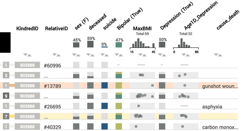
bioRxiv preprint first posted online Apr. 19, 2017; doi: http://dx.doi.org/10.1101/128579. The copyright holder for this preprint
     (which was not peer-reviewed) is the author/funder, who has granted bioRxiv a license to display the preprint in perpetuity.
                                    It is made available under a CC-BY-NC 4.0 International license.

between the supernodes, and visualize the attributes of these nodes in         employs a force directed layout that considers similar phenotypes as
small, embedded visualizations.                                                additional attracting forces. Tuttle et al. [48] use an H-tree layout for
   Small multiples are also commonly used to visualize attributes on           scalable genealogy visualization, with the founder at the center and
top of graphs. Barsky et al. [5] and Lex et al. [29], for example, use         successive generations radiating out based on a fractal pattern. Ball [3]
small multiples to show gene expression data on top of biological              employs the idea to not represent generations as discrete units but use
networks. Using small multiples for multivariate networks, however,            time to position the nodes, and also to draw a person’s life span.
has the disadvantage that the individual networks have to be rendered              Genealogy visualization tools for animal genealogies face a differ-
in less space, limiting their readability and/or the size of the graph for     ent set of challenges compared to those for human genealogies, as
which they are useful for.                                                     the number of descendants sired by individual animals can be large,
   Separate, linked views excel at visualizing the attributes and the          and complex interbreeding is common. Consequently, tree-based ap-
graph individually, but do not support the integration of both well. Sys-      proaches are not well suited for these genealogies. Examples include
tems that use this approach [44, 28] rely on linking and brushing to           CoVE [10], and VIPER [40]. VIPER introduces a sandwich view, that
associate a node with the representation of its attribute, which signifi-      CoVE also adopts. The sandwich view scales well to many descendants
cantly hinders the simultaneous analysis of topology and attributes.           of an individual, but only explicitly encodes the relationships between
   The fourth approach to multivariate graph visualization is to adapt         parents and their children. More distant relationships can be revealed
the layout of the network so that the nodes can be easily associated           through highlighting. Helium [45] is a visualization techniques for
with an effective attribute visualization. This is taken to the extreme in     plant genealogies, which commonly have complex crossing. It uses
GraphDice [8], where nodes are positioned in a series of scatterplots          color coding and scaling of nodes to encode up to two attributes.
purely based on attribute values. Gentler approaches are various lin-              GeneaQuilts [9] is a matrix based technique where each row con-
earization strategies, where graphs are laid out such that associated          stitutes a person and each column a nuclear family. In early stages
attributes can be visualized in efficient tabular layouts, overcoming the      of our design process we considered using a GeneaQuilt instead of
drawbacks of completely separated linked views. Typically, trade-offs          our node link design, since GeneaQuilts produces a linearization of
between optimizing for the readability of the topology and the linear          the graph that would be suitable to associate attributes. We ultimately
layout have to be made. Meyer et al. [34] manually linearize a complete        decided against it because our design for aggregation is more suitable
network and render attributes next to the linear layout. While this is         for node-link diagrams.
an efficient approach, the complexity of the networks for which this is            A different approach to analyzing relatedness is to calculate “kinship
feasible is limited, and topological structures can be hard to see. Partl      coefficients” between individuals, i.e., to calculate path-based metrics
et al. [39] use interaction to extract paths from a network, linearize         for relatedness and visualize them in a matrix [26]. While this is
these paths, and associate the nodes in the paths with rows in a tabu-         scalable, it is not suitable for reasoning about all patterns of inheritance.
lar visualization. This, however, requires interaction and works only              A related tool that is concerned with visualizing phenotypes of
for selected subsets of the graph. The recently published Pathfinder           patient cohorts is PhenoStacks by Glueck et al. [18]. PhenoStacks uses
system [38] uses path queries on networks and presents the resulting           a similar tabular approach as we do for our table.
paths in a linear, ranked list, juxtaposed with rich attribute data. This
approach, however, is only sensible for tasks related to paths.
   Our work falls into the category of adapting the layout by lineariza-       5   V ISUALIZING A M ULTIVARIATE T REE -L IKE G RAPH
tion. We leverage the fact that the genealogical graphs our collaborators      The tasks our collaborators need to address rely heavily on both the
are interested in are tree-like and linearize the positioning of the nodes     familial information contained in the genealogy graph, i.e., the topology,
in the tree. We use this tree to juxtapose scalable and perceptually effi-     and the myriad of attributes associated with individuals (see Section 3).
cient visualizations of the attributes. While there are many approaches        Of the strategies for linearization introduced in Section 4.1, only the
that do this for the leaves in a tree, such as juxtaposing dendrograms         linearization method enables an integrated analysis of topology and
with a heatmap [13], we are not aware of prior tree linearization ap-          attribute at the scale of attributes we are interested in. However, none of
proaches that also visualize attributes for intermediate nodes.                the described linearization methods are suitable for the data and tasks
                                                                               of our collaborators. Here, we introduce a linearization method for
4.2 Genealogy Visualization                                                    tree-like graphs. We define tree-like graphs as rooted, directed graphs
Genealogical charts, as shown in Figure 2, are widely used in genetic          that contain cycles. The purpose of the linearization is to associated the
counseling and the literature on genetic diseases. While they are well         nodes with rows in a table visualization.
suited to visualize a single phenotype of interest, they are not suitable to      A consequence of the linearization strategy is that the layout is not
map a complex phenotype to the node. Our collaborators currently use           as compact as other, common layouts are. To address this issue, we also
Progeny [42], a commercial genealogy drawing tool that closely follows         introduce degree-of-interest based aggregation strategies that integrate
the standard for visualizing genealogies [7, 6] (see the supplementary         seamlessly with the linearized graph.
material for an example figure created with Progeny). While Progeny is            We illustrate this concept here using general, tree-like graphs, for
well suited to draw these standard genealogies for use in presentations,       now ignoring specific properties of genealogies. We later show in
it is ill-suited for exploratory tasks, mainly because of its inability to     Section 6 that this approach extends to genealogies (where each person
efficiently encode attributes in the graph.                                    has two roots — their parents) with minor modifications, and also
    Interactive genealogy visualization tools that are designed to ana-        elaborate on design decisions we made that are specific to our data and
lyze disease clusters and to see disease propagation within families           application area.
include PedVizApi [14], CraneFoot [36], Haploview [4], PediMap [50],
and HaploPainter [47]. HaploPainter [47] visualizes genealogies and
                                                                               5.1 Linearization Approach
genetic recombination events below the individuals’ nodes. While it
shares the approach of showing metadata as rows associated with nodes             De-Cycling In a first step, we remove cycles from the directed
with Lineage, it does not take a linearization approach to make values         graph, transforming it into a tree, by duplicating the node that completes
of different generations easy to compare, it does not aggregate the net-       a cycle, similar to the approach by Mäkinen et al. [36]. If the duplicated
work, and it does not visualize different types of attributes. McGuffin        node has children, we attach all children to one instance, while the other
and Balakrishnan [32], describe layout algorithms for complicated ge-          instance remains a leaf. Figure 3(a) shows a tree-like graph with one
nealogical trees, but also introduce aggregation methods for sub-trees,        cycle, Figure 3(b) shows the resulting tree, where node 7 is duplicated.
which we adopt.                                                                While this duplication strategy works for general directed graphs, it
    Among tools that don’t use the standard genealogical drawing con-          is most useful for directed graphs with a defined root and few cycles,
ventions are Fan Charts [12], which uses the SunBurst technique to             as in these cases most of the topology is retained, and the number of
visualize genealogical trees, and the work by Mazeikla et al. [31], which      additional nodes are negligible with respect to scalability.
bioRxiv preprint first posted online Apr. 19, 2017; doi: http://dx.doi.org/10.1101/128579. The copyright holder for this preprint
(which was not peer-reviewed) is the author/funder, who has granted bioRxiv a license to display the preprint in perpetuity.
It is made available under a CC-BY-NC 4.0 International license.
8
4 8
4
4 8 4 8
* 7*
7
* 3
1 3 1 3 7 3 4 8
7*
7* 7* 7*
6 6 3
2 6 2 6
7* 7*
5 5
5
1 2 5 1 2 5 6
2
1 (a) (b)
(a) (b) (c)
Fig. 4. Aggregation approaches demonstrated using the tree in Fig-
Fig. 3. De-cycling and linearization. (a) A directed, rooted graph with ure 3(c). A black fill indicates a node-of interest. (a) Attribute-preserving
one cycle ending in node 7. (b) We remove the cycle by duplicating the aggregation. Each node of interest (shown in black) is in a separate row.
last node in the cycle (node 7). (c) The tree is linearized so that each Branches without nodes of interest are aggregated into one row, yet all
node is assigned a distinct row. Leaves are rendered above their parents. attributes are preserved in the aggregate representations in the table.
This row-based, linear layout enables an unambiguous, position-based Notice how the two children of node 2 that are not affected are shown
association with a table visualizing attributes. using an implicit encoding, which we refer to as a “kid grid”. (b) Attribute-
hiding aggregation. The branches leading to nodes of interest are hidden
Linearization In most tree layouts [1], associating the nodes with behind them. Only nodes of interest and branches with no nodes of inter-
est have a row of their own. Only the nodes of interest are represented
rows in a table by position is impossible. The tree in Figure 3(b) is
in the table.
compact, yet would require, for example, curved links to associate the
nodes with a table row. To make this association between nodes and
rows of a table intuitive, we use a linearization strategy that assigns
every node a distinct vertical position (i.e., a “row”). The position of Attribute-Preserving Aggregation Here we introduce an aggre-
the node alone thus unambiguously associates the node with a row in gation strategy for linearized layouts that preserves both the structure
a table (see Figure 3(c)). Note that while we assume a left-to-right of the tree and the attributes of all the nodes. Nodes of interest are
tree layout here, a top-to-bottom layout would work equally well for assigned a row of their own, while other nodes are aggregated into a
associating a tree with table columns. single row. Figure 4(a) shows an example of this strategy applied to
Linearized tree layouts are based on tree traversal strategies. While the tree shown in Figure 3(c). This emphasize the nodes of interest,
various strategies, such as breath-first (level-order), or in-order depth- while preserving both, the structure of the graph and the attributes of
first-search are possible, we found that pre-order depth-first search the other nodes.
works well for our purposes, as it results in a crossing-free layout and Our algorithm recursively follows a (sub)tree down a branch by
keeps leaves in subsequent rows. assigning a new row to each inner branch. Inner branches are branches
that don’t end in a leaf after the first edge, i.e., an edge that directly
Following the in-order strategy, we recursively place the descendants
connects to a leaf is not an inner branch. If no node of interest is
of a given node directly above them. Note that a top-down strategy
encountered, it continues to the leaves, placing all nodes of the branch
would be equally possible. We assume that an order of leaves can be
in the same row. Multiple leaves that are not of interest are placed
defined, e.g., based on the attributes. If not, using a random order is
in a “kid grid”, an implicit encoding of the leaves as small nodes to
possible.
the right of their parent. An example is visible in the bottom branch
Figure 3(c) illustrates the results of this algorithm when applied to
in Figure 4(a), where nodes 1, 2, 5, and 7 are on the same row, and
the tree in Figure 3(b) and also shows how to easily associate a table
the leaves (5, 7) are in a kid grid. If a node of interest is encountered,
with the tree. Note that the duplicate node also is duplicated in the
we distinguish two cases. If the node of interest has children that are
associated table.
leaves and that are not nodes of interest themselves, they are added
to a kid grid, which is placed in the next row (see node of interest 3
5.2 Aggregation and its descendant (node 7) that is placed in a kid grid in Figure 4(a)).
While linearizing the tree allows for a direct, position-based association If the node has children that are inner nodes, the algorithm is applied
of the nodes and their attributes, the resulting layout uses more space recursively.
than a compact layout. However, due to their hierarchical structure, The result of this algorithm is a layout that has N rows, where N is
trees are well suited for aggregation. Degree of interest (DOI) func- the sum of:
tions [15] have been widely applied to trees. In our design, we use the • the number of nodes of interest,
generalized idea of degree of interest functions by Furnas [15, 16]. • the number of inner branches that do not end in nodes of interest
We let analysts define a degree of interest function based on the (case for node 4 in Figure 4(a)),
attributes of the nodes, which we call the phenotype of interest (POI). • the number of nodes of interest that have children that are leaves
Nodes that have the POI are referred to as nodes of interest. In contrast (case for the child of node 3 in Figure 4(a)).
to the original formulation of a degree of interest, our POI function is The result in the associated table visualization is that each node of
binary (i.e., a node is either of interest or not) and does not consider interest has a separate row, and the aggregated branches are represented
a distance to a selected node. An example for a POI is “committed in aggregated rows. In practice, we use visual encodings for aggregates
suicide”, which would make all nodes representing individuals that and individual rows that can faithfully represent the data but are also
committed suicide to be considered of interest, or “has a maximum comparable. For details on the table design, see Section 6.2.
BMI of higher than 30”, which would consider all obese individuals to
be of interest. Naturally, POIs that are compound of multiple attributes Attribute-Hiding Aggregation This form of aggregation also pre-
(high BMI and suicide) are possible. serves the complete structure of the tree, but does not preserve attributes
Based on this degree of interest function, we introduce two different of nodes that are not of interest. The results, illustrated in Figure 4(b), is
approaches to aggregation that vary in how they trade-off compactness a scalable approach that can be used to address tasks that are only con-
and preserving the attributes of the nodes: (1) attribute-preserving cerned with the attributes of the nodes of interest and their connectivity,
aggregation, and (2) attribute-hiding aggregation. These aggregation but not with the attributes of the other nodes.
approaches can, of course, not only be applied to the whole tree, but to The main difference compared to the attribute-preserving aggrega-
selected sub-trees, and can also be combined. tion is that nodes of interest are not assigned to a new row when theybioRxiv preprint first posted online Apr. 19, 2017; doi: http://dx.doi.org/10.1101/128579. The copyright holder for this preprint
(which was not peer-reviewed) is the author/funder, who has granted bioRxiv a license to display the preprint in perpetuity.
It is made available under a CC-BY-NC 4.0 International license.
(b)
(a) (b)
(c)
Fig. 6. Different POI functions applied to the same, aggregated sub-
tree. (a) Suicide, as a categorical POI. (b) Age < 40 as a numerical,
thresholded POI.
(a)
The modifications to the layout algorithm to accommodate couples
(d) (e) are minor: couples are always placed in consecutive rows, to avoid
long, vertical parent edges. When one of the spouses has offspring
Fig. 5. Different aggregation cases. (a-c) A family where one woman has with multiple partners, we place all partners in consecutive rows. In
children with two men. One of the children committed suicide. (a) No case of two partners, we place the person with multiple relationships in
aggregation: every person is in their own row. (b) Attribute aggregation: the center to avoid edge crossings. Figure 5(a), for example, shows a
the suicide case is in its own row; the rest of the family is aggregated. woman who had children with two different partners. For more than two
Notice the family grid with two male and one female parents, and one
spouses, however, or spouses who had children with different partners
daughter and one son. The second son is not in the kid grid because he
in alternating order, edge crossings are often unavoidable. Similar to
is a node of interest. (c) Attribute hiding: the family is hidden behind the
suicide case, only the attributes of the suicide case will be shown in the
Mäkinen et al. [36], we use arrows to indicate that a node is duplicated
table. (d-e) A different family, where the node of interest has children, and to point towards the duplicate. To resolve any ambiguities, we draw
leading to special cases. (d) Attribute aggregation: the spouses and an edge connecting the duplicates when hovering over the arrow (see
children are moved to their own row, the line connecting spouses spans supplementary material, Figure S3).
two rows. (e) Attribute hiding: the spouses are placed to the left of the In contrast to traditional genealogical graphs, we do not lay the
suicide case, the children to the right. nodes out by generation, but use the birth year to position the nodes hor-
izontally [3], as shown in Figure 1. This avoids ambiguities about the
birth order and encodes a vital attribute directly in the graph. We also
are encountered. The algorithm again recursively follows a (sub)tree use curved splines instead of the traditional orthogonal edge routing,
down a branch by assigning a new row to each inner branch. If no because continuous edges are easier to follow [51].
nodes of interest are encountered while traversing the branch, the leaves Aggregation Layouts With respect to aggregation, the algorithm
are placed in a kid grid. If a node of interest is encountered, the next is only extended by first looking for spouses before descending into a
step depends on whether it has children that are inner nodes or not. For subtree. If both spouses are nodes of interest, each spouse is assigned
the node’s children that are leaves, a kid grid is used, but no new row is their own row.
started. For all other branches, the algorithm is applied recursively. We previously introduced the concept of kid grids for aggregated
The resulting layout has M rows, where M is the sum of: nodes. Indicating hidden nodes using a glyph has been done before
• the number of inner branches, for graph layouts, most notably by McGuffin and Balakrishnan [32],
• the number of nodes of interest that have at least one child that is who use dots to indicate children in genealogical graphs. Our layout
an inner node. for aggregated genealogies, however, goes beyond a basic indication
Here, only nodes of interest and inner branches that do not end in a of existing nodes as they encode both, topological information and
node of interest are assigned their own row. For consistency, we do not attributes. First, we extend the notion of a kid grid that encodes children,
represent branches that do not end in a node of interest in the table. to a family grid that encodes all members of a family. Figure 5 shows
multiple examples. A family is separated by a vertical line into parents
6 L INEAGE D ESIGN and children. This vertical line represents the line used to connect
Here we describe the design decisions that are specific to the use spouses in unaggregated mode. Parents are placed on the left of the
case of visualizing genealogies and that we realized in the Lineage line. In addition to the node shape, we also redundantly encode sex by
prototype. To address the tasks of our collaborators, Lineage provides position, placing the nodes representing males on top and the nodes
four views, shown in Figure 1: the genealogy graph view and the representing females below. This redundant encoding is useful, as
closely synchronized table view; a data selection view, which can be aggregated nodes are rendered significantly smaller, and hence, can be
used to select which attributes to display; and a family selection view, harder to read. In families with multiple partners, we place all partners
which allows analysts to switch between or select multiple families. in the same family grid, so that, for example, a family where a woman
who has children with three partners is represented by three squares on
6.1 Genealogy Graph top, and one circle at the bottom.
An important difference between genealogical trees and general trees is It is important to note that we break with the convention of placing
that nodes have not one but two parents. To address this, we introduce nodes based on their birth-year for aggregated families. Instead, we
the concept of a couple, indicated by a line connecting the partners (see place the whole family based on the birth year of the parent with a
Figure 5(a)). As is common in genealogical graph layouts, the children blood relationships to the ancestors.
of a relationship then connect to the line representing the couple instead Encoding Attributes in the Graph While we address the prob-
of directly to the parents. We also adopt some of the conventions for lem of encoding multiple attributes for nodes using our linearization
drawing genealogical graphs: males are drawn as rectangles, females approach, direct, on-node encoding of a very small number of attributes
as circles. Deceased individuals are crossed out. Nodes that have the provides the best bridge between attribute-based and topology-based
phenotype of interest are filled-in. tasks. We already discussed how sex (shape), deceased/alive (crossed
As discussed in the previous section, the phenotype of interest can out), birth year (horizontal position), and POI (fill) is encoded directly
be defined dynamically, either based on (combinations of) categorical in the graph. To enable our collaborators to view an additional variable
values, or by brushing a range of a numerical variable. Figure 6 shows in the graph, we introduce a glyph, rendered to the right of the nodes,
the effect of two different POI functions on the same subtree. as shown in Figure 7. In case the attribute is categorical we color-codebioRxiv preprint first posted online Apr. 19, 2017; doi: http://dx.doi.org/10.1101/128579. The copyright holder for this preprint
(which was not peer-reviewed) is the author/funder, who has granted bioRxiv a license to display the preprint in perpetuity.
It is made available under a CC-BY-NC 4.0 International license.
(a) (b)
Fig. 7. Attributes encoded directly in the graph. Age lines visualize the
life-span of individuals. Age lines for people that are alive continue until
the present. Age lines of deceased individuals are terminated at their
year of death. We can see that the individual represented by the node
of interest died at age 31, and his spouse died only shortly thereafter.
Selected attributes can be visualized next to the nodes in glyphs (green
rectangles). (a) The categorical variable bipolar disorder is encoded by a
dark-green color. (b) The numerical variable number of bipolar diagnoses
is encoded as a bar chart.
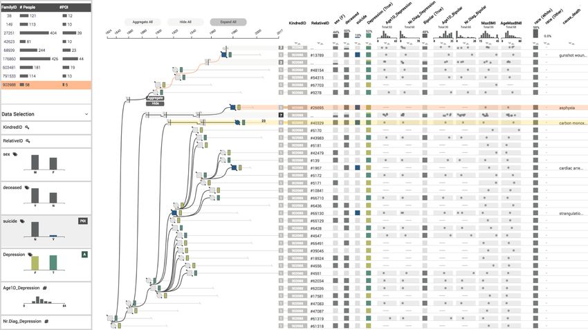
Fig. 9. The table is sorted by suicide, which causes the rows in the table
to be in a different order than the rows in the graph. The association
between the two is retained by the curves connecting them.
Missing values, which are very common in our datasets, are rendered
as a dash and to distinguish them from zero or false values.
We also provide a column that shows how many people are in a given
row. Here, we print the exact number and use a redundant encoding by
value, where darker cells correspond to more individuals in a row.
As we avoid color to encode data, we can employ it to highlight
elements of interest, such as to highlight selected rows and to indicate
the column that encodes the user-selected phenotype of interest and the
primary attribute. In Figure 8, the selected attribute (bipolar) and the
POI (suicide) are rendered in color.
The attributes visualized in the table can be chosen using the data
panel shown in Figure 1. Numerical and categorical attributes listed in
Fig. 8. The table view. The first column encodes how many individu- the panel are accompanied by a histogram, so that analysts can judge
als are aggregated in that row. Binary categories are represented as what to expect before adding an attribute to the table.
present/absent (e.g., sex). Aggregates of categorical variables show In combination with the graph, these features enable analysts to
the proportions of the variable in stacked bars. Numerical values are address the tasks related to analyzing individuals (T2), and comparing
encoded using a dot plot, which is also used for aggregates.
cases (T3).
the glyph; for numerical attributes we show a small bar. In both cases, Finally, we also allow analysts to sort the table based on any column.
the color coding is also used in the table to highlight the relationship This enables analysts to easily identify clusters of similar items (T4).
(see the matching colors for biploar disorder in Figures 7(a) and 8). However, sorting by attribute removes the close association with the
When data is not available for a node, no glyph is shown. graph. To partially remedy this, we draw slope charts, similar to what
is used in LineUp [21], to relate the rows of the table to the rows of the
Finally, we also encode the age of individuals directly in the graph
graph. These connection lines work well for a small number of rows,
by drawing a line from the node, which is placed at the year of birth, to
but often result in significant crossings when dealing with many rows.
the year of death, or to the current year (see Figure 7). These age lines
In that case, interactive highlighting helps to trace the lines. Figure 9
conveniently encode an important variable in the existing coordinate
shows an example of a partially aggregated graph sorted by suicide.
system. We found that the age lines also help to perceptually connect
the nodes to the rows in the table. As we don’t draw age lines for
aggregates, we found it necessary to indicate the connection to the table 6.3 Viewing Multiple Families
using a light-gray background, as can be seen, for example, in Figure 6. One important aspect of our collaborators’ workflow is to compare
multiple families (T5). A requirement for comparison of families is the
6.2 Table Visualization ability to select families T1, which is enabled by the family selection
view, shown at the top left in Figure 1. The family selection view
The attribute table is designed to visualize both rows representing
shows statistics about the family, such as its size, and the number of
individuals and aggregates representing multiple individuals in the same
people with the currently selected POI. It also allows analysts to sort by
space. As shown in Figure 8, we use dot plots to encode numerical
these attributes to, for example, quickly identify how many individuals
data. Combined with transparency and jitter, dot plots can also be used
were diagnosed as bipolar before committing suicide, across the whole
to encode aggregate rows.
dataset, and thus enables them to quickly scan for enriched phenotypes.
For categorical values, we distinguish between binary categories,
Multiple families are seamlessly integrated into the graph and table
such as deceased or alive, and multi-valued categories, such as race.
views (see Figure 10).
We encode binary categories in a single column, as can be seen for “sex
(f)”, where a dark cell corresponds to true and a light cell corresponds
to false. For multi-valued categories, we use one column for each value 7 I MPLEMENTATION AND P RE -P ROCESSING
instead of, e.g., using color. Hence, we use the strongest visual variable Lineage is open source and is implemented in TypeScript as a Caleydo
— position — to encode the data. We represent aggregates of binary or Phovea client/server application [20] and uses D3 for rendering. The
categorical values as stacked bars, which are scaled according to the server component is based on Flask and is provided as a Docker con-
number of individuals in a category. tainer for easy deployment. A prototype of Lineage is available at
Text labels and IDs do not have adequate visual representations http://lineage.caleydoapp.org, the source code is avail-
for groups of elements, so we display an ellipsis (...) for aggregates. able at https://github.com/caleydo/lineage.bioRxiv preprint first posted online Apr. 19, 2017; doi: http://dx.doi.org/10.1101/128579. The copyright holder for this preprint
(which was not peer-reviewed) is the author/funder, who has granted bioRxiv a license to display the preprint in perpetuity.
It is made available under a CC-BY-NC 4.0 International license.
Bipolar Obese
Daughter
Father
Fig. 10. Three suicide cases from two families that are both, bipolar and obese. The family structure reveals that the female case had a father who
also committed suicide at a young age, but for whom no detailed data is available. This suggests an important genetic component.
The prototype made available publicly uses two different datasets: interesting, because she is also obese, has also been diagnosed with
a synthetic dataset designed to showcase features and to highlight depression and committed suicide at a young age. Looking at the
edge cases; and ten selected and anonymized families from the sui- family structure of this case, she realizes that the father of the case
cide study based on data from the Utah Population Database. The has also committed suicide many years before, at about the same age
anonymization method and the selection of families was approved by as the case of interest (see Figure 10). She speculates that, while
the Utah Resource for Genetic and Epidemiologic Research (RGE). no detailed information is available for the father, he likely had the
The anonymization process involves randomizing the sex of individ- same comorbidities and hypothesizes that a genetic factor might be
uals, randomizing the birth and death years, and randomly deleting contributing to these cases. Hence, she chooses to select these three
individuals, in addition to omitting attributes that could be identifiable. cases to analyze their shared genomic regions, to see whether they share
Hence, we do not recommend to make clinical inferences based on the common variants that may alter gene function or regulation and lead
data provided. to risk, with variant selection informed by the knowledge of the case
phenotypes.
8 U SAGE S CENARIO
9 A NALYST F EEDBACK
In a typical usage scenario, analysts want to use Lineage to identify
interesting phenotypes that are familially correlated with suicide. Such We ran an informal feedback session with four analysts (two faculty
discovery will (1) enable selection of familial cases for genotyping members, one research scientist, and one PhD student). With the
and/or sequencing efforts and subsequent genetic risk discovery analy- exception of one of the faculty members, who is also a co-author,
ses, or (2) post-hoc description of cases already subjected to genetic the participants did not contribute to the design and development of
analyses who show significant familial sharing of genomic regions, Lineage, except for the requirement analysis as described in Section 3.
allowing for potential prioritization of genes within these regions based After an introduction to Lineage, participants were asked to use the tool
on genetic associations with co-occurring phenotypes. In this usage with their own data and articulate their thought process and observations
scenario, an analyst starts with a family and browses for cases that are according to the think aloud protocol. This was followed by a brief
bipolar. She discovers two cases in a family with 10 suicides in total. interview. The sessions took between 90 minutes and two hours.
Upon closer investigation, she finds that both cases are male, committed The feedback we received was overwhelmingly positive, including
suicide around the age of 25, were also diagnosed with depression and statements such as “This is going to completely change how we do
were both obese. Looking closer at the number of diagnoses of bipolar things”. One analyst noted that Lineage will allow them to properly use
disorder, she finds that one of the two was diagnosed multiple times, visualization for exploration of genealogies for the first time, because
indicating that the diseases was a significant burden. Exploring the their current tools are not suitable for discovery, as they can only
family structure, she sees that they are related to each other, but not effectively visualize one or two attributes at the same time, and the
too closely, which is promising for a familial genetic analysis, as they tools are essentially static and difficult to use.
might share a relevant gene variant, but will not have the large amount The analysts consistently noted that the integration of attributes and
of genomic sharing of close relatives. By checking the LabID, she family structure is critical for them to make decisions about where to
ensures that she has genetic material in the study for these cases. follow up with subsequent analysis, making comments such as “I think
Next, she adds other families with bipolar suicide cases. One other it’s really helpful to see the attributes next to the graph. It really helps
family has three bipolar cases, but one of these cases seems especially to pinpoint the important cases”.bioRxiv preprint first posted online Apr. 19, 2017; doi: http://dx.doi.org/10.1101/128579. The copyright holder for this preprint
(which was not peer-reviewed) is the author/funder, who has granted bioRxiv a license to display the preprint in perpetuity.
It is made available under a CC-BY-NC 4.0 International license.
We also observed that the analysts largely followed a pattern: after they study contain between 5-15% suicide cases. For these conditions,
they selected a family, they quickly aggregated it to get an overview of we found the resulting layouts to be very compact and useful.
the data. Then they continued to drill down, using selective expansion We found Lineage to scale well to families with about 1500 individ-
of branches. After a while, they turned to the table and began to sort uals, which covers most families in our collaborators dataset (547 out
by attributes, to look for individuals with interesting phenotypes. Mul- of 550 families have less than 1000 individuals). We also experimented
tiple analysts commented that a hierarchical sorting approach, which with the largest families in our dataset, which contain about 2500 in-
is currently not supported, would be useful, so that they can easily dividuals. For these families, we observe several seconds of wait time
find people with a complex phenotype. When using the sorting, they until the de-cycling and the layout is computed. We anticipate to be
frequently used the row-highlight feature to trace individuals in the able to address these performance limitations through pre-computing
table back to the genealogy. They also commented that highlighting and caching initial layouts.
the paths to shared ancestors would be very helpful in these cases. In terms of the scalability of the visual encodings, we argue that
We asked the analysts about their opinions on attribute-preserving Lineage produces a more readable layout in less space than Progeny, the
aggregation and how it compared to attribute-hiding aggregation. They tool that is currently used by our collaborators for displaying genealo-
commented that attribute-preserving aggregation is not particularly gies. Note that Progeny has only very limited capabilities of showing
useful for their suicide dataset due to the sparse attributes of the non- attributes by encoding attributes directly on the nodes, and displaying
affected individuals, but that they can imagine it to be very useful text underneath nodes, and attributes cannot be dynamically selected or
when applied to their autism dataset that contains more data on family manipulated. For a comparison between Progeny and Lineage, please
members. One analyst gave the example that he would be interested to refer to the supplementary material. When using suicide as a POI (the
see autism spectrum scores aggregated for a whole family. most common use case) and when using attribute-hiding aggregation,
The analysts also stated that they believe that Lineage graphs are a family with about 400 individuals fits onto a single screen without
appropriate for presentations in publications and presentations, as the scrolling (see Supplementary Figure S2). Larger families, attribute-
visual encodings are easy to explain. They asked for some features in preserving aggregation, or no aggregation more commonly require
support of presentations, such as the ability to hide irrelevant branches scrolling.
and/or nodes of the graph, or to re-define the founder to clean up the The number of attributes that can be displayed for each individual
genealogy. Finally, we also asked for other features that they wished is limited by the horizontal screen size. On a large, 2560x1600 pixel
the tool had. The answers to that were mostly regarding data, i.e., to display, about 20-40 dimensions can be shown, depending on the type
load more data into the tool and to provide export capabilities for a (text and numerical columns need more space than binary categorical,
subsequent statistical analysis. for example). We found that this typically exceeds the number of
attributes our collaborators would like to study simultaneously.
10 D ISCUSSION
We argue that our linearization and attribute-driven aggregation ap- 11 C ONCLUSION AND F UTURE W ORK
proach can be applied broadly when analyzing multivariate trees or In this paper, we introduced a novel approach for visualizing multi-
tree-like graphs, such as phylogenies or file directories. We also believe variate trees and tree-like graphs using a linearization approach. We
that our strategy of combining explicit, node-link layouts, with the demonstrate the usefulness of our approach by realizing it in the Lin-
implicit layout of the family grids is transferable to other application eage system, which is designed for the visualization of genealogies in a
scenarios. clinical context.
Our described linearization approach makes the association between
While Lineage in its current form is already highly useful to our
nodes and attributes obvious and enables a tight integration of attribute-
collaborators, there are many directions in which it could be extended.
based and topology-based graph analysis tasks. Both aggregation
Specifically, we currently deal only with a selected subset of the 3000
methods described serve to reduce the space usage of the linearized
dimensions that are available for each of our cases. We plan to develop
tree while preserving the topology, and while preserving the desired
integrated visual and analytical methods to select dimensions of interest
level of information about the attributes. The aggregation is based on
for any given subset of patients. For example, the system could identify
two principles: assigning nodes to be aggregated to the same row, and
that for a given family, PTSD is a common comorbidity and suggest to
combining the explicit node-link layout with the implicit encoding for
the analyst to add PTSD to the table. This kind of approach is going to
aggregated nodes and their leaves (family grids).
be especially important when we start to integrate the detailed genetic
The Lineage genealogy visualization tool specifically can be broadly data that is available for many of these cases.
used with other genealogical datasets, e.g., to study autism, diabetes,
or cancer. There are many groups at the University of Utah that make
use of the Utah Population Database, and we have already established ACKNOWLEDGMENTS
contact to other potential collaborators who are in need of a clini- We thank Asmaa Aljuhani and Annie Cherkaev for their contributions.
cal genealogy visualization tool. Some of these datasets also have We also thank our collaborators and the Visualization Design Lab
detailed attributes for non-affected cases, which will make our attribute- at the University of Utah for the feedback, and the Caleydo team
preserving aggregation approach even more valuable. for their technical support. This work was supported in part by the
While our data is unique with respect to its scope, detailed ge- US National Institutes of Health (U01 CA198935, R00 HG007583,
nealogical datasets are becoming more common, as they have shown R01MH099134) and the DoD - Office of Economic Adjustment (OEA),
immense potential for population genetics [30]. We believe that our ST1605-16-01. We thank the Pedigree and Population Resource of the
approach could also be adapted to datasets containing many small fami- Huntsman Cancer Institute, University of Utah (funded in part by the
lies (siblings, parents, grandparents, of affected individuals) as they are Huntsman Cancer Foundation) for its role in the ongoing collection,
commonly collected to study the genetic disease of one family member. maintenance and support of the Utah Population Database (UPDB).
We also acknowledge partial support for the UPDB through grant P30
Scalability In contrast to other tools, such as the DOITree [22] our CA2014 from the National Cancer Institute, and from the University
aggregation approach preserves all of the structure of the tree. This of Utah’s Program in Personalized Health and Center for Clinical and
is suitable for trees with hundreds of nodes, but not for trees with Translational Science.
tens of thousands of nodes or more. To scale to larger trees, these
algorithms could be combined with hiding parts or the tree. Also,
while the described algorithms work for any tree and any phenotype R EFERENCES
of interest, they are most efficient if the number of nodes of interest is [1] R. Adrian. Tree Drawing Algorithms. In Handbook of Graph Drawing
small compared to the number of nodes in total. A common phenotype and Visualization, pages 155–192. CRC Press, 2013. Google-Books-ID:
of interest for our collaborators is suicide, and the typical genealogies lQBrAAAAQBAJ.You can also read