Does Twitter language reliably predict heart disease? A commentary on Eichstaedt et al. (2015a)
←
→
Page content transcription
If your browser does not render page correctly, please read the page content below
Does Twitter language reliably predict
                               heart disease? A commentary on
                               Eichstaedt et al. (2015a)
                               Nicholas J.L. Brown and James C. Coyne
                               University Medical Center, University of Groningen, Groningen, Netherlands

                                   ABSTRACT
                                   We comment on Eichstaedt et al.’s (2015a) claim to have shown that language patterns
                                   among Twitter users, aggregated at the level of US counties, predicted county-level
                                   mortality rates from atherosclerotic heart disease (AHD), with ‘‘negative’’ language
                                   being associated with higher rates of death from AHD and ‘‘positive’’ language
                                   associated with lower rates. First, we examine some of Eichstaedt et al.’s apparent
                                   assumptions about the nature of AHD, as well as some issues related to the secondary
                                   analysis of online data and to considering counties as communities. Next, using the data
                                   files supplied by Eichstaedt et al., we reproduce their regression- and correlation-based
                                   models, substituting mortality from an alternative cause of death—namely, suicide—as
                                   the outcome variable, and observe that the purported associations between ‘‘negative’’
                                   and ‘‘positive’’ language and mortality are reversed when suicide is used as the outcome
                                   variable. We identify numerous other conceptual and methodological limitations that
                                   call into question the robustness and generalizability of Eichstaedt et al.’s claims, even
                                   when these are based on the results of their ridge regression/machine learning model.
                                   We conclude that there is no good evidence that analyzing Twitter data in bulk in this
                                   way can add anything useful to our ability to understand geographical variation in AHD
                                   mortality rates.

                               Subjects Epidemiology, Health Policy, Psychiatry and Psychology, Public Health, Statistics
Submitted 6 March 2018         Keywords Heart disease, Risk factors, Well-being, Big data, Artifacts, Emotions, Social media,
Accepted 28 August 2018        False positives, Language
Published 21 September 2018
Corresponding author
Nicholas J.L. Brown,           INTRODUCTION
nicholasjlbrown@gmail.com
                               Eichstaedt et al. (2015a) claimed to have demonstrated that language patterns among
Academic editor
Tjeerd Boonstra                Twitter users, aggregated at the level of US counties, were predictive of mortality rates
Additional Information and     from atherosclerotic heart disease (AHD) in those counties, with ‘‘negative’’ language
Declarations can be found on   (expressing themes such as disengagement or negative relationships) being associated
page 18
                               with higher rates of death from AHD and ‘‘positive’’ language (e.g., upbeat descriptions
DOI 10.7717/peerj.5656         of social interactions or positive emotions) being associated with lower AHD mortality.
    Copyright                  Eichstaedt et al. examined a variety of measures to demonstrate the associations between
2018 Brown and Coyne           Twitter language patterns and AHD, including (a) the frequency of usage of individual
Distributed under              words associated with either positive or negative feelings or behaviors, (b) the tendency of
Creative Commons CC-BY 4.0     Twitter users to discuss ‘‘positive’’ (e.g., skilled occupations) or ‘‘negative’’ (e.g., feelings of
OPEN ACCESS                    boredom) topics, and (c) an omnibus model incorporating all of their Twitter data, whose

                               How to cite this article Brown and Coyne (2018), Does Twitter language reliably predict heart disease? A commentary on Eichstaedt et al.
                               (2015a). PeerJ 6:e5656; DOI 10.7717/peerj.5656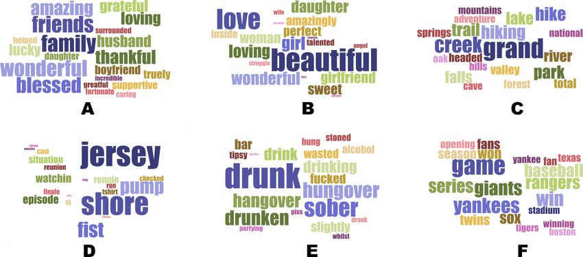
performance they compared with one using only ‘‘traditional’’ predictors such as health
                                 indicators and demographic and socioeconomic variables.
                                    The claims made by Eichstaedt et al. (2015a) attracted considerable attention in the
                                 popular media (e.g., Izadi, 2015; Jacobs, 2015; Singal, 2015), with many of these articles
                                 being based in large part on the Association for Psychological Science’s (2015) own press
                                 release. However, a close examination of Eichstaedt et al.’s article and data appears to
                                 reveal a number of potential sources of distortion and bias in its assumptions about the
                                 nature of AHD, the use of Twitter data as a proxy for the socioemotional environment and
                                 people’s health, and the use of counties as the unit of analysis. Some of these problems are
                                 immediately obvious from reading Eichstaedt et al.’s article, while others only manifested
                                 themselves in the testing of the relevant data that we undertook.
                                    Here, we first present a selection of the main problems that we identified when reading
                                 Eichstaedt et al.’s (2015a) article. We then expose further problems that emerged after we
                                 scrutinized the original data and also cross-validated the application of Eichstaedt et al.’s
                                 models to a different mortality outcome variable, namely suicide. We end with a discussion
                                 of some broader implications for the use of large-scale sources of data to draw conclusions
                                 about health and human behavior based on sophisticated computer models.

                                 Issues related to the idea of psychological causes of AHD
                                 Perhaps a large part of the appeal of Eichstaedt et al.’s (2015a) claims about the potential for
                                 community-level psychological factors—notably, those that purportedly lead Twitter users
                                 to either make aggressive or otherwise anti-social outbursts, or, conversely, express upbeat
                                 and positive sentiments—to somehow affect local rates of death from AHD is that these
                                 claims echo the common belief, repeated in the first sentence of Eichstaedt et al.’s abstract,
                                 that hostile or highly stressed individuals are more susceptible to cardiovascular problems.
                                 The notion that a loudmouthed, dominating, aggressive person is somehow more likely to
                                 suddenly drop dead from a heart attack is widespread in lay or pop psychology thinking
                                 (e.g., Riggio, 2014), perhaps at least in part because it provides some comfort to people
                                 on the receiving end of such individuals’ behavior. Indeed, although Eichstaedt et al. did
                                 not use the term ‘‘Type A personality’’ in their article, this stereotype—characterized by a
                                 tendency towards aggression and a variety of other negative interpersonal characteristics,
                                 as well as greater susceptibility to cardiovascular problems—is a staple part of the popular
                                 culture surrounding the relation between mental and physical health (e.g., Wilson, 2009).
                                 Yet despite initial promising findings suggesting a link between Type A behavior pattern
                                 (TABP) and cardiac events and mortality in small samples (Friedman & Rosenman, 1959),
                                 an accumulation of evidence from more recent large-scale studies has consistently failed
                                 to show reliable evidence for such an association (Kuper, Marmot & Hemingway, 2002).
                                 Appearances of positive findings could be generated using a range of distress or negative
                                 affectivity variables (Smith, 2006). However, it was then recognized that negative affectivity
                                 could not readily be separated from a full range of antecedent and concurrent biological,
                                 psychological, and social factors. At best, negative affectivity is likely to be no more than
                                 a non-informative risk marker (Ormel, Rosmalen & Farmer, 2004), not a risk factor for

Brown and Coyne (2018), PeerJ, DOI 10.7717/peerj.5656                                                                       2/21
AHD. Its apparent predictive power is greatly diminished with better specification and
measurement of confounds (Smith, 2011).
A recent large scale study of over 150,000 Australians (Welsh et al., 2017) provides a
typical example of the problem. Significant associations between levels of psychological
distress and incidence of ischemic heart disease (a superordinate category in the ICD-10
classification that includes AHD as a subcategory) decreased as adjustments were made
for demographic and behavioral characteristics until measurement error and residual
confounding seemed to account for any remaining association. As the authors put it, ‘‘A
substantial part of the distress–IHD association is explained by confounding and functional
limitations . . . . Emphasis should be on psychological distress as a marker of healthcare
need and IHD risk, rather than a causative factor’’ (Welsh et al., 2017, p. 1).
In contrast to TABP, socioeconomic conditions have long been identified as playing a
role in the development of AHD. For example, Clark et al. (2009) noted the importance
of access to good-quality healthcare and early-life factors such as parental socioeconomic
status. However, no county-level measure of either of those variables appeared in Eichstaedt
et al.’s (2015a) model or data set.
Issues related to the etiology of AHD
As the single most common ICD-10 cause of mortality in the United States, AHD might
have seemed like a natural choice of outcome variable for a study such as that of Eichstaedt
et al. (2015a). However, it is important to take into account some aspects of the nature
and course of AHD. It is a chronic disease that typically develops asymptomatically over
decades. The first recognition of AHD often follows an event such as an acute myocardial
infarction or some other sudden incident, reflecting the fact that the cumulative build-up
of plaque over time has finally caused a blockage of the arteries (Funk, Yurdagul Jr & Orr,
2012) rather than any specific change in the immediately preceding time period. Indeed,
disagreement among physicians as to whether the cause of death is AHD or some other
cardiac event is common (Mant et al., 2006). A definitive post-mortem diagnosis of AHD
may require an autopsy, yet the number of such procedures performed in the United States
has halved in the past four decades (Hoyert, 2011).
In contrast to AHD, there is another cause of death for which the existence of an
association with the victim’s recent psychological state is widely accepted, namely suicide
(Franklin et al., 2017; O’Connor & Nock, 2014). Although suicide can be the result of
long-term mental health problems and other stressors, a person’s psychological state in
the months and days leading up to the point at which they take their own life clearly has a
substantial degree of relevance to their decision. Hence, we might expect any county-level
psychological factors that act directly on the health and welfare of members of the local
community to be more closely reflected in the mortality statistics for suicide than those for
a chronic disease such as AHD.
Issues related to the secondary analysis of data collected online
In the introduction to their article, Eichstaedt et al. (2015a) invoked Google’s use of search
queries related to influenza, ‘‘providing earlier indication of disease spread than the
Brown and Coyne (2018), PeerJ, DOI 10.7717/peerj.5656 3/21Centers for Disease Control and Prevention’’ (p. 160) as a (presumably positive) example
of how ‘‘digital epidemiology can support faster response and deeper understanding of
public-health threats than can traditional methods’’ (p. 160). However, both Google’s
project to infer a relation between searches for certain terms and the immediate prevalence
of an acute infectious disease, and Eichstaedt et al.’s attempt to correlate certain kinds
of communication with chronic cardiovascular conditions, suffer from the fundamental
problem that they are attempting to extract some kind of signal from what may very well
be a large amount of noise. In fact, before it was quietly shut down in August 2015, Google
Flu Trends (GFT) failed—in some cases spectacularly—to correctly predict the seasonal
spread of influenza in the United States on several occasions. As Lazer et al. (2014) put
it, in their review of the problems that beset GFT, ‘‘The core challenge is that most big
data that have received popular attention are not the output of instruments designed to
produce valid and reliable data amenable for scientific analysis’’ (p. 1203)—a remark that
clearly also applies to the notionally random selection of tweets that constitute the Twitter
‘‘Garden Hose’’ data, especially since, as we show below, this selection may not have been
entirely random.
As well as the limitations noted in Eichstaedt et al.’s article (2015a) and Supplemental
Material (2015b)—such as the difference in Twitter user density across counties, and the fact
that 7% of tweets were mapped to the wrong county—we note that there is also a potential
source of bias in the geographical coding of their Twitter data, namely the assumption that
the users who provided enough information to allow their tweets to be associated with
a county represented an unbiased sample of Twitter users in that county. This requires
people of all ages, genders, socio-economic status levels, and ethnic backgrounds to be
equally likely to either list their city and state in their profile, or to enable geotagging of
their Tweets. However, it seems entirely plausible that certain categories of individuals
might be more likely to self-censor their profile information than others (for example, it
could be that people who do not wish to reveal their location are more or less restrained in
their use of hostile language). Given that only 16% of tweets could be mapped to counties,
any bias in this area could have substantial consequences.
Issues associated with considering counties as communities
As Eichstaedt et al. (2015a) p. 160 themselves noted, ‘‘Counties are the smallest
socioecological level for which most CDC health variables and US Census information are
available.’’ Thus, these authors seem to have acknowledged that their use of counties as
their unit of analysis was driven principally by (eminently reasonable) practical constraints.
However, Eichstaedt et al.’s subsequent interpretation of their results (e.g., ‘‘language
expressed on Twitter revealed several community-level psychological characteristics
that were significantly associated with heart-disease mortality risk,’’ p. 164) requires
that counties also constitute meaningful communities. Indeed, this interpretation also
implies that any psychological mechanism that might account for the relation between
the vocabulary of Twitter users and the health outcomes of the wider population within
any given county works in a similar way across all counties. Yet there seem to be several
reasons to question such assumptions. First, the size and population of US counties varies
Brown and Coyne (2018), PeerJ, DOI 10.7717/peerj.5656 4/21widely; both their land areas (ranging from 1.999 to 144,504.789 square miles) and their
2010 populations (from 82 to 9,818,605) span five orders of magnitude. Second, across the
United States, the political and economic importance of counties as a level of government
(between the municipality and state level) is highly variable, being generally greater in the
South (Benton, 2002, p. 7; Haider-Merkel, 2009, p. 723); indeed, in Connecticut, Rhode
Island, and much of Massachusetts, counties have no governmental function whatsoever.
Third, it is not clear that many Americans identify at all closely with their county as a
source of community (Kilgore, 2012). Fourth, within counties, socioeconomic and other
factors often vary enormously:
[I]n New York County, New York, . . . neighborhoods range from the Upper East Side
and SoHo to Harlem and Washington Heights. . . . [I]n San Mateo County, California,
. . . neighborhoods range from the Woodside estates of Silicon Valley billionaires to the
Redwood City bungalows of Mexican immigrants. (Abrams & Fiorina, 2012, p. 206)
Given such diversity in the scale and sociopolitical significance of counties, we find it
difficult to conceive of a county-level factor, or set of factors, that might be associated
with both Twitter language and AHD prevalence with any degree of consistency across
the United States. Eichstaedt et al. (2015a, p. 166) cited two meta-analyses (Leyland, 2005;
Riva, Gauvin & Barnett, 2007), which they claimed provided support for the idea that ‘‘the
aggregated characteristics of communities . . . account for a significant portion of variation
in health outcomes,’’ but both of those meta-analyses were based predominantly on small
and relatively homogeneously-sized geographical areas (and Leyland’s study examined
only health-related behaviors, not outcomes). The approximate population of each area
in Leyland’s study was 5,000, while Riva, Gauvin & Barnett (2007) reported a median area
population of 8,600; compare these with Eichstaedt et al.’s mean county population of
206,000 and median of 78,000. As Beyer, Schultz & Rushton (2008, p. 40) put it, ‘‘The county
often represents an area too large to use in determining true, local patterns of disease.’’
Working with aggregated data sets, such as Eichstaedt et al.’s (2015a) county-level data,
also raises the question of whether specific data items can be aggregated in a meaningful
way to create a collective ‘‘characteristic’’ (cf. Subramanian et al., 2008). For example,
it is difficult to know what interpretation to place on the median individual household
income of a county, especially one with a highly diverse population. It is also worth noting
that, as reported by Eichstaedt et al. in their Supplemental Tables document (2015c), the
‘‘county-level’’ data for all of the variables that measure ‘‘county-level’’ health in their study
(obesity, hypertension, diabetes, and smoking) are in fact statistical estimates derived from
state-level data using ‘‘Bayesian multilevel modeling, multilevel logistic regression models,
and a Markov Chain Monte Carlo simulation method’’ (p. DS7). However, Eichstaedt et
al. provided no estimates of the possible errors or biases that the use of such techniques
might introduce.
Based on the above observations, we decided to reproduce a number of Eichstaedt et
al.’s (2015a) analyses, using their original data files in conjunction with other sources of
information, to see whether the assumptions made by these authors stand up to a critical
examination.
Brown and Coyne (2018), PeerJ, DOI 10.7717/peerj.5656 5/211 An earlier version of the present article, METHOD
available in preprint form at https:
//psyarxiv.com/dursw, stated that we had We were able to download all of Eichstaedt et al.’s (2015a) data files from the relevant
not been able to obtain Eichstaedt et al.’s Open Science Foundation (OSF) repository, and the majority of the analyses that follow
(2015a) code because it had not been made
available in the same OSF repository as the are based on these data.1 We did not have access to the original Twitter ‘‘Garden Hose’’
data. We are happy to acknowledge here data set, so our analyses rely on the summaries of word usage provided by Eichstaedt et al.
that Eichstaedt and colleagues had in fact
made their code available on the website in their data files.
of their Differential Language Analysis Next, we downloaded county-aggregated, age-adjusted mortality data for 2009 and 2010
ToolKit (DLATK) software project, a fact
that they have now documented in their for the ICD-10 category I25.1 (atherosclerotic heart disease) from the Centers for Disease
recent preprint (Eichstaedt et al., 2018). Control and Prevention (CDC) online public health database, known as Wonder (http:
We followed the installation instructions
for DLATK and were able to reproduce //wonder.cdc.gov/), in order to check that we could reproduce Eichstaedt et al.’s (2015a)
the analyses described by Eichstaedt et data set exactly. We also downloaded comparable mortality data for the ICD-10 categories
al. (2015a, p. 161) under the heading of
‘‘Predictive models’’. X60–X84, collectively labeled ‘‘Intentional self-harm’’—in order to test the idea that suicide
might be at least as well predicted by Twitter language as AHD—as well as the data for several
other causes of death (including all-cause mortality) for comparison purposes. Finally, we
obtained data about the precise geographical locations of counties from the US Census
Bureau (http://www.census.gov/geo/www/gazetteer/files/Gaz_counties_national.zip). All
of our statistical analyses were performed in R; a copy of the analysis code can be found at
https://osf.io/g42dw.
RESULTS
Using data downloaded from the CDC Wonder database, we were able to reproduce
Eichstaedt et al.’s (2015a) principal data file, named countyoutcomes.csv, exactly. We were
also able to reproduce Eichstaedt et al.’s reported numerical results from their article
to within rounding error using our own R code (for the dictionary and topic language
variables) or by running their modeling software in a virtual machine environment (for
the analyses under the heading of ‘‘Predictive models’’).
In the following sections, we report a number of findings that we made when exploring
Eichstaedt et al.’s (2015a) data set and the other data that we obtained. The order of these
sections follows the same structure that we used in the introduction of the present article,
showing how these findings relate to the concerns that we expressed earlier under three
broad headings: (a) the use of mortality from AHD as the outcome variable; (b) the use of
county-level aggregated data; and (c) the use of patterns of language in posts to Twitter as
the principal predictor of the outcome.
Variability in ICD-10 coding of cause of death
The validity of the mortality data from the CDC, and in particular the ICD-10 coding
of the cause of death, is crucial to establishing the validity of Eichstaedt et al.’s (2015a)
findings. Examination of the mortality figures from the counties included in Eichstaedt et
al.’s study shows that death rates from AHD in 2009–2010 ranged from 13.4 per 100,000
people (1.55% of all recorded deaths) in East Baton Rouge Parish, LA to 185.0 per 100,000
people (26.11% of all recorded deaths) in Richmond County, NY. It is not clear that
any county-level environmental, economic, or social factors that might contribute to
Brown and Coyne (2018), PeerJ, DOI 10.7717/peerj.5656 6/21the development of AHD would be sufficient to explain why this condition—which, as
Eichstaedt et al. noted, is the single most prevalent ICD-10 cause of mortality in the United
States—appears to cause 13.8 times more deaths in one county than another. The two
counties just mentioned are both among the 10% most populous counties in the US,
with a total of 7,001 and 6,907 deaths, respectively, being recorded there in 2009–2010;
this suggests that the large difference in recorded mortality from AHD is unlikely to be
a statistical fluke due to a limited sample. In contrast, for deaths from cancer, the range
of per-county mortality rates across the 1,347 counties included by Eichstaedt et al. runs
from 102.4 to 326.7 per 100,000 people—a factor of 3.19 from lowest to highest, which is
little different from the range for all-cause mortality (478.8 to 1,390.3 per 100,000 people, a
factor of 2.90 from lowest to highest). Eichstaedt et al.’s acknowledgement that ‘‘the coding
on death certificates may be inconsistent’’ (p. 166) would thus appear to be somewhat of an
understatement, at least as far as AHD is concerned. Indeed, it seems possible that at least
part of the variance in AHD mortality (whether this is to be explained by ‘‘community-level
psychological characteristics’’ or some other mechanism) might be due, not to differences
in the actual prevalence of AHD as the principal cause of death, but rather to variations in
the propensity of local physicians to certify the cause of death as AHD (McAllum, St. George
& White, 2005; Messite & Stellman, 1996; Stausberg et al., 2006). Researchers who intend to
study AHD mortality using county-level data may wish to take this possibility into account
(cf. Roth et al., 2017).
Use of mortality from AHD as the outcome variable
The chronic nature of AHD implies that, to the extent that its prevalence may be affected
by deleterious or protective lifestyle and social factors—including Eichstaedt et al.’s (2015a,
p. 164) purported ‘‘indicators of community-level psychosocial health’’—it will have been
necessary for these factors to have exerted their effects over a long period. However, there
are two potential sources of discrepancy between the current psychosocial state of a person’s
county of residence and its past effects on their health. First, the socioeconomic climate of
an area can change substantially in less than a generation. The decline in the fortunes of
the city of Detroit provides a recent dramatic example of this (LeDuff, 2014), but economic
development can also bring rapid positive change to parts of a state within quite a short
time. Second, individuals tend not to stay in one place; the county where someone spends
his or her childhood may be a long way from where he or she ends up working, and possibly
different again from where the same person is living when symptoms of AHD emerge later
in life, which might be after retirement. Data from the US Census Bureau (2011) show
that in 2010 approximately 3.5% of Americans moved either to another county in the
same state, or to another state altogether, a figure that appears from an examination of
comparable data from other years to be relatively constant over time. Thus, it seems likely
that a substantial proportion of the people who die from AHD each year in any given
county may have lived in one or more other counties during the decades when AHD was
developing, and thus been exposed to different forms, both favorable and unfavorable,
of Eichstaedt et al.’s purported community-level psychological characteristics during that
period.
Brown and Coyne (2018), PeerJ, DOI 10.7717/peerj.5656 7/21Table 1 Correlations between self-harm and Twitter language measured by dictionaries.
Language variable r p 95% CI
Risk factors
Anger −0.169Figure 1 Twitter topics highly correlated with age-adjusted mortality from self-harm, cf. Eichstaedt
et al.’s (2015a). Figure 1 (A–C) Topics positively correlated with county-level self-harm mortality: (A)
Friends and family, r = .175. (B) Romantic love, r = .176. (C) Time spent with nature, r = .214. (D–F)
Topics negatively correlated with county-level self-harm mortality: (D) Watching reality TV, r = −.200.
(E) Binge drinking, r = −.249. (F) Baseball, r = −.317.
Full-size DOI: 10.7717/peerj.5656/fig-1
−.317, CI = [−.381, −.251]), binge drinking (e.g., drunk, sober, hungover; r = −.249,
CI = [−.316, −.181]), and watching reality TV (e.g., Jersey, Shore, episode; r = −.200, CI =
[−.269, −.130]). All of the correlations between these topics and self-harm outcomes, both
positive and negative, were significant at the same Bonferroni-corrected significance level
(i.e., .05/2,000 = .000025) used by Eichstaedt et al. (2015a), and remained significant at that
level after adjusting for income and education. That is, several topics that were ostensibly
associated with ‘‘positive,’’ ‘‘eudaimonic’’ approaches to life predicted higher rates of
county-level self-harm mortality, whereas apparently hedonistic topics were associated
with lower rates of self-harm mortality, and the magnitude of these associations was at least
as great—and in a few cases, even greater—than those found by Eichstaedt et al. These topics
are shown in ‘‘word cloud’’ form (generated at https://www.jasondavies.com/wordcloud/)
3 In
in our Fig. 1 (cf. Eichstaedt et al.’s (2015a) Figure 1).
their recent preprint, Eichstaedt et al.
(2018) noted that the relation between This would seem to pose a problem for Eichstaedt et al.’s (2015a, p. 166) claim to have
self-harm and positive Twitter language shown the existence of ‘‘community-level psychological factors that are important for the
disappeared when they added measures
of county-level rurality and elevation as cardiovascular health of communities.’’ Apparently the ‘‘positive’’ versions of these factors,
covariates. We do not find this surprising. while acting via some unspecified mechanism to make the community as a whole less
Our point is not that Twitter language
actually predicts county-level mortality susceptible to developing hardening of the arteries, also simultaneously manage to make
from suicide (or AHD); rather, it is that the inhabitants of those counties more likely to commit suicide, and vice versa. We suggest
with a sufficient number of predictors,
combined with unreliability in the that more research into the possible risks of increased levels of self-harm might be needed
measurement of these, one can easily find before ‘‘community-level psychological factors’’ were to be made the focus of intervention,
spurious relations between variables (cf.
Westfall & Yarkoni, 2016).
as Eichstaedt et al. suggested in the final sentence of their article.3
Bias caused by selection of counties
As noted above, the CDC Wonder database returns county-aggregated mortality data for
any given cause of death only for those counties where at least 10 deaths from that cause were
recorded per year, on average, during the period covered by the user’s request. This cutoff
Brown and Coyne (2018), PeerJ, DOI 10.7717/peerj.5656 9/21means that Eichstaedt et al.’s (2015a) data set is skewed toward counties having higher rates
of AHD. For example, AHD mortality was sufficiently high in Plumas County, CA (2010
population 20,007; 25 deaths from AHD in 2009–2010) for this county to be included,
whereas the corresponding prevalence in McKinley County, NM (2010 population 71,492;
17 deaths from AHD in 2009–2010), as well as 130 other counties with higher populations
than Plumas County but fewer than 20 deaths from AHD, was not. Thus, the selection
of counties tends to include those with higher levels of the outcome variable, which has
the potential to introduce selection bias (Berk, 1983). For example, counties with a 2010
population below the median (78,265) in Eichstaedt et al.’s data set had significantly
higher AHD mortality rates than counties with larger populations (53.21 versus 49.87
per 100,000; t (1344.6) = 3.12, p = .002, d = 0.17). The effect of such bias on the rest of
Eichstaedt et al.’s analyses is hard to estimate, but given that one of these authors’ headline
results—namely, that their Twitter-only model predicted AHD mortality ‘‘significantly
better’’ than a ‘‘traditional’’ model, a claim deemed sufficiently important to be included
in their abstract—had an associated p value of .049, even a very small difference might be
enough to tilt this result away from traditional statistical significance.
Problems associated with county-level aggregation of data
We noted earlier that the diversity among counties made it difficult to imagine that the
relation between Twitter language and AHD would be consistent across the entire United
States. Indeed, when the counties in Eichstaedt et al.’s (2015a) data set are split into two
equal subsets along the median latitude of their centroids (38.6484 degrees North, a line
that runs approximately through the middle of the states of Missouri and Kansas), the
purported effect of county-level Twitter language on AHD mortality as measured by
Eichstaedt et al.’s dictionaries seems to become stronger in the northern half of the US than
for the country as a whole, but mostly disappears in the southern half (see our Table 2).
There does not appear to be an obvious theoretical explanation for this effect; if anything
one might expect the opposite, in view of the observation made previously that counties
may play a greater role in people’s lives in the South.
A further issue with Eichstaedt et al.’s (2015a) use of data aggregated at the level of
counties is that it resulted in an effective sample size that was much smaller than these
authors suggested. For example, Eichstaedt et al. compared their model to ‘‘[t]raditional
approaches for collecting psychosocial data from large representative samples . . . [which]
are based on only [emphasis added] thousands of people’’ (p. 166). This suggests that these
authors believed that their approach, using data that was generated by an unspecified (but
implicitly very large) number of different Twitter users, resulted in a more representative
data set than one built by examining the behaviors and health status of ‘‘only’’ a few
thousand individuals. However, by aggregating their Twitter data at the county level, and
merging it with other county-level health and demographic information, Eichstaedt et al.
reduced each of their variables of interest to a single number for each county, regardless
of that county’s population. In effect, Eichstaedt et al.’s data set contains a sample of
only 1,347 individual units of analysis, each of which has the same degree of influence
on the conclusions of the study. A corollary of this is that, despite the apparently large
Brown and Coyne (2018), PeerJ, DOI 10.7717/peerj.5656 10/21Table 2 Partial correlations between atherosclerotic heart disease (AHD) mortality and Twitter language measured by dictionaries, across the
northern and southern halves of the United States.
North South
Language variable Partial r p 95% CI Partial r p 95% CI
Risk factors
Anger 0.240words on Twitter suggests that they are in relatively common usage—as are the words
‘‘Jew[s]’’ and ‘‘Muslim[s].’’ In Appendix B of their recent preprint, Eichstaedt et al. (2018)
have indicated that they were previously unaware of this issue, which we therefore presume
reflects a decision by Twitter to bowdlerize the ‘‘Garden Hose’’ dataset. Such a decision
clearly has substantial consequences for any attempt to infer a relation between the use
of hostile language on Twitter and health outcomes, which requires that the tweets being
analyzed are truly representative of the language being used. Indeed, it could be argued
that there are few better examples of language that expresses interpersonal hostility than
6 We assume that the apparent omission of
‘‘Jew[s]’’ and ‘‘Muslim[s]’’ was motivated
invective directed towards ethnic or religious groups.6
by concerns that at least some of the
tweets mentioning these words might be Potential sources of bias in the “Topics” database
expressing hostility towards these groups.
A further potential source of bias in Eichstaedt et al.’s (2015a) analyses, which these authors
did not mention in their article or their supplemental documents (Eichstaedt et al., 2015b;
Eichstaedt et al., 2015c), is that their ‘‘Topics’’ database was derived from posts on Facebook
(i.e., not Twitter) by a completely different sample of users, as can be seen at the site from
which we downloaded this database (http://wwbp.org/data.html). Furthermore, some
7 Itappears that the relative size of the
of the topics that were highlighted by Eichstaedt et al. in the word clouds7 in their Fig. 1
words in Eichstaedt et al.’s (2015a, Fig. 1) contain words that appear to directly contradict the topic label (e.g., ‘‘famous’’ and ’’lovers’’
word clouds is determined by the relative
frequency of these words in the Facebook
in ‘‘Hate, Interpersonal Tension,’’ left panel; ‘‘enemy’’ in ‘‘Skilled Occupations,’’ middle
data from which the topics were derived, panel; ‘‘painful’’ in ‘‘Positive Experiences,’’ left panel). There are also many incorrectly
and does not represent the prevalence of
these words in the Twitter data.
spelled words, as in topic #135 (‘‘can’t, wait, afford, move, belive [sic ], concentrate’’),
topic #215 (‘‘wait, can’t, till, tomorrow, meet, tomarrow [sic ]’’), topic #467 (‘‘who’s, guess,
coming, thumbs, guy, whos [sic ], idea, boss, pointing’’), and many topics make little
sense at all, such as #824 (‘‘tooo, sooo, soooo, alll, sooooo, toooo, goood, meee, meeee,
youuu, gooo, soooooo, allll, gooood, ohhh, ughhh, ohhhh, goooood, mee, sooooooo’’)
and #983 (‘‘ur, urself, u’ll, coz, u’ve, cos, urs, bcoz, wht, givin’’). The extent to which these
automatically extracted topics from Facebook really represent coherent psychological or
social themes that might appear with any frequency in discussions on Twitter seems to
be questionable, in view of the different demographics and writing styles on these two
networks.
Flexibility in interpretation of dictionary data
A problem for Eichstaedt et al.’s (2015a) general argument about the salutary effects of
‘‘positive’’ language was the fact that the use of words expressing positive relationships
appeared, in these authors’ initial analyses, to be positively correlated with AHD mortality.
To address this, Eichstaedt et al. took the decision to eliminate the word love from their
dictionary of positive-relationship words. Their justification for this was that ‘‘[r]eading
through a random sample of tweets containing love revealed them to be mostly statements
about loving things, not people’’ (p. 165). However, similar reasoning could be applied
to many other dictionary words—including those that featured in results that did not
contradict Eichstaedt et al.’s hypotheses—with the most notable among these being,
naturally, hate. In fact, it turns out that hate dominated Eichstaedt et al.’s negative
relationships dictionary (41.6% of all word occurrences) to an even greater degree than love
Brown and Coyne (2018), PeerJ, DOI 10.7717/peerj.5656 12/21did for the positive relationships dictionary (35.8%). We therefore created an alternative
version of the negative relationships dictionary, omitting the word hate, and found that,
compared to the original, this version was far less likely to produce a statistically significant
regression model when predicting AHD mortality (e.g., regressing AHD on negative
relationships, controlling for income and education: with hate included, partial r = .107,
pTwitter-predicted AHD mortality. Eichstaedt et al. (2015a, p. 164) claimed that ‘‘a high
degree of agreement is evident’’ between the two maps. We set out to evaluate this claim
by examining the color assigned to each county on each of the two maps, and determining
the degree of difference between the mortality rates corresponding to those colors. To
this end, we wrote a program to extract the colors of each pixel across the two maps,
convert these colors to the corresponding range of AHD mortality rates, and draw a new
map that highlights the differences between these rates using a simple color scheme. The
color-based scale shown at the bottom of Eichstaedt et al.’s Figure 3 seems to imply that the
maps are composed of 10 different color codes, each representing a decile of per-county
AHD mortality, but in fact this scale is somewhat misleading. In fact, 14 different colors
(plus white) are used for the counties in the maps in Eichstaedt et al.’s Figure 3, with
each color apparently (assuming that each color corresponds to an equally-sized interval)
9 More precisely, 200 counties (32.9%) representing around seven percentile rank places, or what we might call a ‘‘quattuordecile,’’
had a discrepancy of three or more color
intervals, while 123 counties (20.2%) had
of the AHD mortality distribution. For more than half (323 out of 608, or 53.1%) of the
a discrepancy of six or more. Assuming for counties that have a color other than white in Eichstaedt et al.’s maps, the difference
simplicity that rounding error is uniformly
distributed, a difference of three intervals
between the two maps is three or more of these seven-point ‘‘color intervals,’’ as shown in
corresponds to a mean difference of our Fig. 2. Within these counties, the mean discrepancy is at least 29.5 percentage points,
21.4 percentage points, and a difference
of six intervals to a mean difference of
and probably considerably higher.9 It is therefore questionable whether it is really the case
42.8 percentage points. Thus, even with that ‘‘[a] high degree of agreement is evident’’ (Eichstaedt et al., 2015a, p. 164) between the
the extremely conservative simplifying
assumption that ‘‘three (six) or more color
two maps, such that one might use the Twitter-derived value to predict AHD mortality for
intervals’’ actually means ‘‘exactly three any practical purpose.
(six) intervals,’’ the mean discrepancy
across these counties is ((200 × 21.4) +
(123 × 42.8)) / 323 = 29.5 percentage DISCUSSION
points. Note also that the possible extent
of the discrepancy is bounded at between In the preceding paragraphs, we have examined a number of aspects of Eichstaedt et al.’s
seven and 13 color intervals, depending on
the relative positions of the two counties
(2015a) claims about the county-level effects of Twitter language on AHD mortality, using
along the 1–14 scale. for the most part these authors’ own data. We have shown that many of these claims
are, at the least, open to alternative interpretations. The coding of their outcome variable
(mortality from AHD) is subject to very substantial variability; the process that selects
counties for inclusion is biased; the same regression and correlation models ‘‘predict’’
suicide at least as well as AHD mortality but with almost opposite results (in terms of the
valence of language predicting positive or negative outcomes) to those found by Eichstaedt
et al.; the Twitter-based dictionaries appear not to be a faithful summary of the words
that were actually typed by users; arbitrary choices were apparently made in some of
the dictionary-based analyses; the topics database was derived from a completely different
sample of participants who were using Facebook, not Twitter; there are numerous problems
associated with the use of counties as the unit of analysis; and the predictive power of the
model, including the associated maps, appears to be questionable. While we were able to
reproduce—at a purely computational level—the results of Eichstaedt et al.’s advanced
prediction model, based on ridge regression and k-fold cross-validation, we do not believe
that this model can address the problems of validity and reliability posed by the majority of
the points just mentioned. In summary, the evidence for the existence of community-level
psychological factors that determine AHD mortality better than traditional socioeconomic
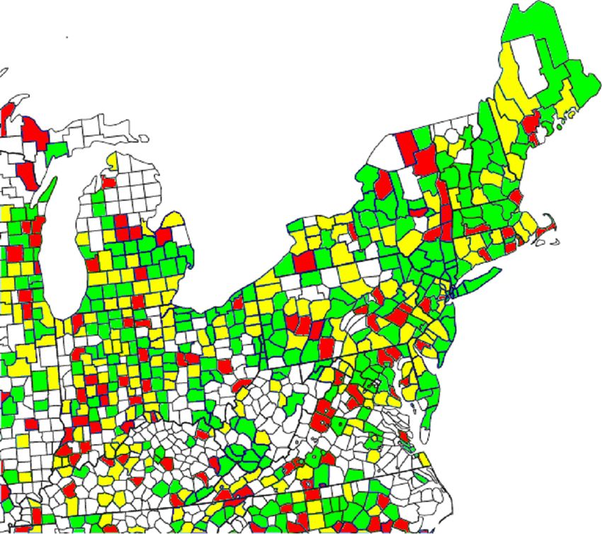
Brown and Coyne (2018), PeerJ, DOI 10.7717/peerj.5656 14/21Figure 2 Difference between the two maps of AHD mortality rates (CDC-reported and Twitter-
predicted) from Eichstaedt et al.’s (2015a) Figure 3. Note: Green indicates a difference of 0–2 color-scale
points (see discussion in the text) between the two maps; yellow, a difference of 3–5 points; red, a
difference of 6 or more points. Of the 608 colored areas, 123 (20.2%) are red and 200 (32.9%) are yellow.
Full-size DOI: 10.7717/peerj.5656/fig-2
and demographic predictors seems to be considerably less strong than Eichstaedt et al.
claimed.
A tourist, or indeed a field anthropologist, driving through Jackson County (2010
population 42,376) and Clay County (2010 population 26,890) in southern Indiana might
not notice very much difference between the two. According to the US Census Bureau
(https://factfinder.census.gov/) these counties have comparable population densities,
ethnic make-ups, and median household incomes. It seems unlikely that there would be a
large variation in the ‘‘norms, social connectedness, perceived safety, and environmental
stress, that contribute to health and disease’’ (Eichstaedt et al., 2015a, pp. 159–160) between
these two rural Midwestern communities. Yet according to Eichstaedt et al.’s data, the levels
of anger and anxiety expressed on Twitter were more than 12 and six times, respectively,
higher in Jackson County than in Clay County. These differences are not easy to explain;
any community-level psychological characteristics that might be driving them must obey
some strange properties. Such characteristics would have to operate, at least partly, in
ways that are not accounted for by variables for which Eichstaedt et al. applied statistical
Brown and Coyne (2018), PeerJ, DOI 10.7717/peerj.5656 15/21controls (such as income and smoking prevalence), yet presumably they must have some
physical manifestation in order to be able to have an effect on people’s expressed feelings.
It is difficult to imagine how such a characteristic might have gone unnoticed until now,
yet be able to cause people living in very similar socioeconomic conditions less than 100
miles apart in the same state to express such varying degrees of negative emotionality. A
more parsimonious explanation, perhaps, is that there is a very large amount of noise in
the measures of the meaning of Twitter data used by Eichstaedt et al., and these authors’
complex analysis techniques (involving, for example, several steps to deal with high
multicollinearity) are merely modeling this noise to produce the illusion of a psychological
mechanism that acts at the level of people’s county of residence. Certainly, the different
levels of ‘‘negative’’ Twitter language between these two Indiana counties appear to have
had no deleterious differential effect on local AHD mortality; indeed, at 45.4 deaths per
100,000 inhabitants, ‘‘angry’’ Jackson County’s AHD mortality rate in 2009–2010 was
23.7% lower than ‘‘laid-back’’ Clay County’s (59.5 per 100,000 inhabitants). As we showed
in our analysis of Eichstaedt et al.’s comparative maps, this failure of Twitter language to
predict AHD mortality with any reliability is widespread.
In a recent critique, Jensen (2017) examined the claims made by Mitchell et al. (2013)
regarding the ability of Twitter data to predict happiness. Jensen argued that ‘‘the extent of
overlap between individuals’ online and offline behavior and psychology has not been well
established, but there is certainly reason to suspect that a gap exists between reported and
actual behavior’’ (p. 2). Jensen went on to raise a number of other points about the use
of Twitter’s ‘‘garden hose’’ dataset that appear to be equally applicable to Eichstaedt et al.
(2015a), concluding that ‘‘When researchers approach a data set, they need to understand
and publicly account for not only the limits of the data set, but also the limits of which
questions they can ask . . . and what interpretations are appropriate’’ (p. 6). It is worth
noting that Mitchell et al. were attempting to predict happiness only among the people
who were actually sending the tweets that they analyzed. While certainly not a trivial
undertaking, this ought to be considerably less complex than Eichstaedt et al.’s attempt
to predict the health of one part of the population from the tweets of an entirely separate
part (cf. their comment on p. 166: ‘‘The people tweeting are not the people dying’’).
Hence, it would appear likely that Jensen’s conclusions—namely, that the limitations of
secondary data analyses and the inherent noisiness of Twitter data meant that Mitchell et
al.’s claims about their ability to predict happiness from tweets were not reliably supported
by the evidence—would be even more applicable to Eichstaedt et al.’s study, unless these
authors could show that they took steps to avoid the deficiencies of Mitchell et al. On a
related theme, Robinson-Garcia et al. (2017) warned that bots, or humans tweeting like
bots, represent a considerable challenge to the interpretability of Twitter data; this theme
has become particularly salient in view of recent claims that a substantial proportion of the
content on Twitter and other social media platforms may not represent the spontaneous
output of independent humans (Varol et al., 2017).
The principal theoretical claim of Eichstaedt et al.’s (2015a) article appears to be that
the best explanation for the associations that were observed between county-level Twitter
language and AHD mortality is some geographically-localized psychological factor, shared
Brown and Coyne (2018), PeerJ, DOI 10.7717/peerj.5656 16/2110 Eichstaedt et al. (2015a) included a
by the inhabitants of an area, that exerts10 a substantial influence on aspects of human
disclaimer about causality on p. 166 of life as different as vocabulary choice on social media and arterial plaque accumulation,
their article. However, we feel that this did
not adequately compensate for some of
independently of other socioeconomic and demographic factors. However, Eichstaedt et al.
their language elsewhere in the article, such did not provide any direct evidence for the existence of these purported community-level
as ‘‘Local communities create [emphasis
added] physical and social environments
psychological characteristics, nor of how they might operate. Indeed, we have shown that
that influence [emphasis added] the the same techniques that predicted AHD mortality could equally well have been used to
behaviors, stress experiences, and health
of their residents’’ (p. 166; both of the
predict county-level suicide prevalence, with the difference that higher rates of self-harm
italicized words here seem to us to imply seem to be associated with ‘‘positive’’ Twitter language. Of course, there is no suggestion
causation at least as strongly as our word
‘‘exerts’’), and ‘‘Our approach . . . could
that the study of the language used on Twitter by the inhabitants of any particular county
bring researchers closer to understanding has any real predictive value for the local suicide rate; we believe that such associations are
the community-level psychological factors
that are important for the cardiovascular
likely to be the entirely spurious results of imperfect measurements and chance factors, and
health of communities and should to use Twitter data to predict which areas might be about to experience higher suicide rates is
become the focus of intervention’’ (p. 166,
seemingly implying that an intervention
likely to prove extremely inaccurate (and perhaps ethically questionable as well). We believe
to change these psychological factors that it is up to Eichstaedt et al. to show convincingly why these same considerations do not
would be expected to lead to a change
in cardiovascular health).
apply to their analyses of AHD mortality; as it stands, their article does not do this. Taken in
conjunction with the pitfalls (Westfall & Yarkoni, 2016) of including imperfectly-measured
11 Forexample, using data from the CDC
for the 2009–2010 period, county- covariates (such as Eichstaedt et al.’s county-level measures of smoking and health status,
level mortality from assault is strongly as described above) in regression models, and the likely presence of numerous substantial
correlated with county-level mortality
from cancer (r = .55), but completely but meaningless correlations in any data set of this type (the ‘‘crud factor’’; Meehl, 199011 ),
uncorrelated with county-level mortality it seems entirely possible that Eichstaedt et al.’s conclusions might be no more than the
from AHD (r = .00). There seems to be no
obvious theoretical explanation for these result of fitting a model to noise.
results.
CONCLUSIONS
It appears that the existence of community-level psychological characteristics—and their
presumed valence, either being ‘‘protective’’ or ‘‘risk’’ factors for AHD mortality—
was inferred by Eichstaedt et al. (2015a) from the rejection of a series of statistical null
hypotheses which, though not explicitly formulated by these authors, appear to be of
the form ‘‘There is no association between the use of (a ‘positive’ or ‘negative’ language
element) by the Twitter users who live in a given county, and AHD-related mortality
among the general population of that county.’’ Yet the rejection of a statistical null
hypothesis cannot in itself justify the acceptance of any particular alternative hypothesis
(Dienes, 2008)—especially one as vaguely specified as the existence of Eichstaedt et al.’s
purported county-level psychological characteristics that operate via some unspecified
mechanism—in the absence of any coherent theoretical explanation. Indeed, it seems to us
that Eichstaedt et al.’s results could probably equally well be used to justify the claim that
the relation between Twitter language and AHD mortality is being driven by county-level
variations in almost any phenomenon imaginable. To introduce a new psychological
construct without a clear definition, and whose very existence has only been inferred from
a correlational study—as Eichstaedt et al. did—is a very risky undertaking indeed.
Brown and Coyne (2018), PeerJ, DOI 10.7717/peerj.5656 17/21ACKNOWLEDGEMENTS
We thank Casper Albers, Daniël Lakens, and a number of colleagues who wished to
remain anonymous for helpful discussions during the writing of this article. All errors and
omissions remain the responsibility of the authors alone.
ADDITIONAL INFORMATION AND DECLARATIONS
Funding
The authors received no funding for this work.
Competing Interests
James C. Coyne is an Academic Editor for PeerJ.
Author Contributions
• Nicholas J.L. Brown conceived and designed the experiments, performed the
experiments, analyzed the data, contributed reagents/materials/analysis tools, prepared
figures and/or tables, authored or reviewed drafts of the paper, approved the final draft.
• James C. Coyne authored or reviewed drafts of the paper, approved the final draft.
Data Availability
The following information was supplied regarding data availability:
Brown, Nicholas JL. 2018. ‘‘Reanalysis of Eichstaedt et al. (2015: Twitter/heart disease).’’
Open Science Framework. February 12. https://osf.io/g42dw/.
REFERENCES
Abrams SJ, Fiorina M. 2012. The Big Sort that wasn’t: A skeptical reexamination.
Political Science & Politics 45:203–210 DOI 10.1017/S1049096512000017.
Association for Psychological Science. 2015. Language on Twitter tracks rates of
coronary heart disease. Available at http:// www.psychologicalscience.org/ news/
releases/ twitter-usage-can-predict-rates-of-coronary-heart-disease.html.
Benton JE. 2002. Counties as service delivery agents: changing expectations and roles.
Westport: Praeger.
Berk RA. 1983. An introduction to sample selection bias in sociological data. American
Sociological Review 48:386–398 DOI 10.2307/2095230.
Beyer KMM, Schultz AF, Rushton G. 2008. Using ZIP R codes as geocodes in cancer
research. In: Rushton G, Armstrong MP, Gittler J, Greene BR, Pavlik CE, West MM,
Zimmerman DL, eds. Geocoding health data: the use of geographic codes in cancer
prevention and control, research, and practice. Boca Raton: CRC Press, 37–67.
Clark AM, DesMeules M, Luo W, Duncan AS, Wielgosz A. 2009. Socioeconomic status
and cardiovascular disease: risks and implications for care. Nature Reviews Cardiology
6:712–722 DOI 10.1038/nrcardio.2009.163.
Dienes Z. 2008. Understanding psychology as a science. Basingstoke: Palgrave Macmillan.
Brown and Coyne (2018), PeerJ, DOI 10.7717/peerj.5656 18/21Eichstaedt JC, Schwartz HA, Giorgi S, Kern ML, Park G, Sap M, Labarthe DR, Larson
EE, Seligman MEP, Ungar LH. 2018. More evidence that Twitter language predicts
heart disease: a response and replication. Available at https:// psyarxiv.com/ p75ku/ .
Eichstaedt JC, Schwartz HA, Kern ML, Park G, Labarthe DR, Merchant RM, Jha S,
Agrawal M, Dziurzynski LA, Sap M, Weeg C, Larson EE, Ungar LH, Seligman
MEP. 2015a. Psychological language on Twitter predicts county-level heart disease
mortality. Psychological Science 26:159–169 DOI 10.1177/0956797614557867.
Eichstaedt JC, Schwartz HA, Kern ML, Park G, Labarthe DR, Merchant RM, Jha S,
Agrawal M, Dziurzynski LA, Sap M, Weeg C, Larson EE, Ungar LH, Seligman MEP.
2015b. Supplemental method. Available at http:// journals.sagepub.com/ doi/ suppl/
101177/ 0956797614557867 .
Eichstaedt JC, Schwartz HA, Kern ML, Park G, Labarthe DR, Merchant RM, Jha S,
Agrawal M, Dziurzynski LA, Sap M, Weeg C, Larson EE, Ungar LH, Seligman MEP.
2015c. Supplemental tables. Available at http:// wwbp.org/ papers/ PsychSci2015_
HeartDisease_Tables.pdf .
Franklin JC, Ribeiro JD, Fox KR, Bentley KH, Kleiman EM, Huang X, Musacchio KM,
Jaroszewski AC, Chang BP, Nock MK. 2017. Risk factors for suicidal thoughts and
behaviors: a meta-analysis of 50 years of research. Psychological Bulletin 143:187–232
DOI 10.1037/bul0000084.
Friedman M, Rosenman R. 1959. Association of specific overt behaviour pattern with
blood and cardiovascular findings. Journal of the American Medical Association
169:1286–1296 DOI 10.1001/jama.1959.03000290012005.
Funk SD, Yurdagul Jr A, Orr AW. 2012. Hyperglycemia and endothelial dysfunction
in atherosclerosis: lessons from type 1 diabetes. International Journal of Vascular
Medicine 2012:569654 DOI 10.1155/2012/569654.
Goudet L. 2013. Alternative spelling and censorship: the treatment of profanities in
virtual communities. In: Jamet D, Jobert M, eds. Aspects of linguistic impoliteness.
Cambridge: Cambridge Scholars, 209–222.
Haider-Merkel D. 2009. Political encyclopedia of US states and regions. New York: CQ
Press.
Hoyert DL. 2011. The changing profile of autopsied deaths in the United States, 1972–
2007 (NCHS data brief no. 67). Hyattsville: National Center for Health Statistics.
Available at https:// www.cdc.gov/ nchs/ data/ databriefs/ db67.pdf .
Izadi E. 2015. Tweets can better predict heart disease rates than income, smoking and
diabetes, study finds. The Washington Post. Available at https:// www.washingtonpost.
com/ news/ to-your-health/ wp/ 2015/ 01/ 21/ tweets-can-better-predict-heart-disease-
rates-than-income-smoking-and-diabetes-study-finds/ .
Jacobs T. 2015. Happier tweets, healthier communities. Pacific Standard. Available at
https:// psmag.com/ environment/ happier-tweets-healthier-communities-98710.
Jensen EA. 2017. Putting the methodological brakes on claims to measure national
happiness through Twitter: methodological limitations in social media analytics.
PLOS ONE 12(9):e0180080 DOI 10.1371/journal.pone.0180080.
Brown and Coyne (2018), PeerJ, DOI 10.7717/peerj.5656 19/21You can also read