Malaise and remedy of binary boson-star initial data
←
→
Page content transcription
If your browser does not render page correctly, please read the page content below
Malaise and remedy of binary boson-star initial data

                                                     Thomas Helfer1 , Ulrich Sperhake1,2,3 , Robin Croft2 , Miren
                                                     Radia2 , Bo-Xuan Ge4 , Eugene A. Lim4
                                                     1 Department of Physics and Astronomy, Johns Hopkins University, 3400 N.
arXiv:2108.11995v1 [gr-qc] 26 Aug 2021

                                                     Charles Street, Baltimore, Maryland 21218, USA
                                                     2 Department of Applied Mathematics and Theoretical Physics, Centre for

                                                     Mathematical Sciences, University of Cambridge, Wilberforce Road, Cambridge
                                                     CB3 0WA, United Kingdom
                                                     3 Theoretical Astrophysics 350-17, California Institute of Technology, 1200 E

                                                     California Boulevard, Pasadena, CA 91125, USA
                                                     4 Theoretical Particle Physics and Cosmology Group, Physics Department,Kings

                                                     College London, Strand, London WC2R 2LS, United Kingdom
                                                     E-mail: thomashelfer@live.de, U.Sperhake@damtp.cam.ac.uk,
                                                     M.R.Radia@damtp.cam.ac.uk, bo-xuan.ge@kcl.ac.uk,
                                                     eugene.a.lim@gmail.com

                                                     Abstract. Through numerical simulations of boson-star head-on collisions, we
                                                     explore the quality of binary initial data obtained from the superposition of
                                                     single-star spacetimes. Our results demonstrate that evolutions starting from a
                                                     plain superposition of individual boosted boson-star spacetimes are vulnerable to
                                                     significant unphysical artefacts. These difficulties can be overcome with a simple
                                                     modification of the initial data suggested in [1] for collisions of oscillatons. While
                                                     we specifically consider massive complex scalar field boson star models up to a
                                                     6th-order-polynomial potential, we argue that this vulnerability is universal and
                                                     present in other kinds of exotic compact systems and hence needs to be addressed.
Malaise and remedy of binary boson-star initial data 2
1. Introduction
The rise of gravitational-wave (GW) physics as an observational field, marked by the
detection of GW150914 [2] and followed by about 50 further compact binary events
[3, 4] over the past years, has opened up unprecedented opportunities to explore
gravitational phenomena. From tests of general relativity [5, 6, 7, 8, 9, 10] to the
exploration of BH populations [11, 12, 13, 14, 15] or charting the universe with
independent new methods [16, 17], GW astronomy offers potential for revolutionary
insight into long-standing open questions; for a review see [18]. Some answers,
such as the association of a soft gamma-ray burst with the neutron star merger
GW170817 [19, 20] have already raised our understanding to new levels. GW physics
furthermore establishes new concrete links to other fields of research, most notably to
particle and high-energy physics and the exploration of the dark sector of the universe
[21, 18]. Two important ingredients of this remarkable connection are the characteristic
interaction of fundamental fields with compact objects through superradiance [22] and
their capacity to form compact objects through an elaborate balance between the
intrinsically dispersive character of the fields and their self-gravitation. The latter
feature has given rise to the hypothesis of a distinct class of compact objects as early
as the 1950s [23]. In contrast to their well known fermionic counterparts – stars, white
dwarfs or neutron stars – these compact objects are composed of bosonic particles or
fields and, hence, commonly referred to as Boson Stars (BS). GW observations provide
the first systematic approach to search for populations of these objects or to constrain
their abundance. As with all other GW explorations, the success of this exploration is
heavily reliant on the availability of accurate theoretical predictions for the anticipated
GW signals. This type of calculation, using numerical relativity techniques [24], is the
topic of this work.
The idea of bosonic stars dates back to Wheeler’s 1955 study of gravitational-
electromagnetic entities or geons [23]. By generalising from real to complex-valued
fundamental fields, it is even possible to obtain genuinely stationary solutions to the
Einstein-matter equations. First established for spin 0 or scalar fields [25, 26, 27], this
idea has more recently been extended to spin 1 or vector (aka Proca‡) fields [28] as
well as wider classes of scalar BSs [29, 30]. In the wake of the dramatic progress of
numerical relativity in the simulations of black holes (BHs) [31, 32, 33] (see [34] for a
review), the modelling of BSs and binary systems involving BSs has rapidly gathered
pace.
The first BS models computed in the 1960s consisted of a massive but non-
interacting complex scalar field ϕ. This class of stationary BSs, commonly referred
to as mini boson stars, consists of a one parameter family of ground-state solutions
characterised by the central scalar-field amplitude that reveals a stability structure
analogous to that of Tolman-Oppenheimer-Volkoff [35, 36] stars: a stable and an
unstable branch of ground-state solutions are separated by the configuration with
maximal mass [37, 38, 39]. For each ground-state model, there furthermore exists a
countable hierarchy of excited states with n > 0 nodes in the scalar profile [40, 41, 42].
Numerical evolutions of these excited BSs demonstrate their unstable character, but
also reveal significant variation in the instability time scales [43].
‡ Even though the term “boson star” generally applies to compact objects formed of any bosonic
fields, it is often used to specifically denote stars made up of a scalar field. Stars composed of vector
fields, in contrast, are most commonly referred to as Proca stars. Unless specified otherwise, we shall
accordingly assume the term boson star to imply scalar-field matter.Malaise and remedy of binary boson-star initial data 3
Whereas mini BS models are limited in terms of their maximum compactness,
self-interacting scalar fields can result in significantly more compact stars, even denser
than neutron stars [44, 45, 46, 47]. This raises the intriguing question whether compact
BS binaries may reveal themselves through characteristic GW emission analogous to
that from BHs or NSs [48]. Recent studies conclude that this may well be within the
grasp of next-generation GW detectors and, in the case of favourable events, even with
advanced LIGO [49, 50, 51].
One of the characteristic properties of BSs is the quantised nature of their spin.
The linearised Einstein equations in the slow-rotation limit lead to a two-dimensional
Poisson equation that does not admit everywhere regular solutions except for trivial
constants; in consequence BSs cannot rotate perturbatively [52]. By relaxing the slow-
rotation approximation, Schunck and Mielke [53] computed the first (differentially)
rotating BSs and found that these solutions have an integer ratio of angular momentum
to particle number. The structure of spinning BS models has been studied extensively
over the years [54, 55, 56, 57, 58, 59, 60, 61, 62]. The quantised nature of the angular
momentum also applies to Proca and Dirac (spin 12 ) stars [63], but numerical studies
of the formation of rotating stars have revealed a striking difference between the
scalar and vector case: while collapsing scalar fields shed all their angular momentum
through an axisymmetric instability, the collapse of vector fields results in spinning
Proca stars with no indication of an instability [64, 50]. This observation is supported
by analytic calculations [65], but the instability may be quenched by self-interaction
terms in the potential function or in the Newtonian limit [66]. For further reviews of
the structure and dynamics of single BSs, we note the reviews [67, 68, 69, 70].
The first simulations of BS binaries have considered the head-on collision of
configurations with phase differences between the constituent stars or opposite
frequencies [71]; see also [72, 73]. The phase or frequency differences manifest
themselves most pronouncedly in the dynamics and GW emission at late times around
merger. These collisions result in either a BH, a non-rotating BS or a near-annihilation
of the scalar field in the case of opposite frequencies. BS binaries with orbital angular
momentum generate a GW signal qualitatively similar to that of BH binaries during
the inspiral phase, but exhibit a much more complex structure around merger [74, 75].
In agreement with the above mentioned BS formation studies, the BS inspirals also
seem to avoid the formation of spinning BSs, although they may settle down into
single nonrotating BSs.
In spite of the rapid progress of this field, the computation of GW templates
for BSs still lags considerably behind that of BH binaries, both in terms of precision
and coverage of the parameter space. Clearly, the presence of the matter fields adds
complexity to this challenge, but also alleviates some of the difficulties through the
non-singular character of the BS spacetimes. The first main goal of our study is
to highlight the substantial risk of obtaining spurious physical results due to the
use of overly simplistic initial data constructed by plain superposition of single-BS
spacetimes. Our second main goal is to demonstrate how an astonishingly simple
modification of the superposition procedure, first identified by Helfer et al. [1] for
oscillatons, overcomes most of the problems encountered with plain superposition.
We summarise our main findings as follows.
(1) An adjustment of the superposition procedure, given by Eq. (45), results in a
significant reduction of the constraint violations inherent to the initial data; see
Fig. 3.Malaise and remedy of binary boson-star initial data 4
(2) In the head-on collision of mini BS binaries with rather low compactness, we
observe a significant drop of the radiated GW energy with increasing distance
d if we use plain superposition. This physically unexpected dependence on the
initial separation levels off only for rather large d & 150 M , where M denotes
the Arnowitt-Deser-Misner (ADM) mass [76]. In contrast, the total radiated
energy computed from the evolution of our adjusted initial data displays the
expected behaviour over the entire studied range 75.5 M ≤ d ≤ 176 M : a very
mild increase in the radiated energy with d. In the limit of large d & 150 M ,
both types of simulations agree within numerical uncertainties; see upper panel
in Fig. 6.
(3) In collisions of highly compact BSs with solitonic potentials, the radiated energy
is largely independent of the initial separations for both initial data types, but
for plain superposition we consistently obtain ∼ 10 % more radiation than for
the adjusted initial data; see bottom panel in Fig. 6. Furthermore, we find plain
superposition to result in a slightly faster infall. The most dramatic difference,
however, is the collapse into individual BHs of both BSs well before merger if we
use plain superposition. No such collapse occurs if we use adjusted initial data.
Rather, these lead to the expected near-constancy of the central scalar-field
amplitude of the BSs throughout most of the infall; see Fig. 9.
(4) We have verified through evolutions of single boosted BSs that the premature
collapse into a BH is closely related to the spurious metric perturbation (44)
that arises in the plain superposition procedure. Artificially adding the same
perturbation to a single BS spacetime induces an unphysical collapse of the
BS that is in qualitative and quantitative agreement with that observed in the
binary evolution starting with plain superposition; see Fig. 9.
The detailed derivation of these results begins in Sec. 2 with a review of the formalism
and the computational framework of our BS simulations. We discuss in more detail in
Sec. 3 the construction of initial data through plain superposition and our modification
of this method. In Sec. 4, we compare the dynamics of head-on collisions of mini BSs
and highly compact solitonic BS binaries starting from both types of initial data. We
note the substantial differences in the results thus obtained and argue why we regard
the results obtained with our modification to be correct within numerical uncertainties.
We summarise our findings and discuss future extensions of this work in Sec. 5.
Throughout this work, we use units where the speed of light and Planck’s constant
are set to unity, c = ~ = 1. We denote spacetime indices by Greek letters running
from 0 to 3 and spatial indices by Latin indices running from 1 to 3.
2. Formalism
2.1. Action and covariant field equations
The action for a complex scalar field ϕ minimally coupled to gravity is given by
√
Z
1 1 µν
S= −g R − [g ∇µ ϕ̄∇ν ϕ + V (ϕ)] d4 x , (1)
16πG 2
where gαβ denotes the spacetime metric and R the Ricci scalar associated with this
metric. The characteristics of the resulting BS models depend on the scalar potentialMalaise and remedy of binary boson-star initial data 5
V (ϕ); in this work, we consider mini boson stars and solitonic boson stars, obtained
respectively for the potential functions
2
|ϕ|2
Vmin = µ2 |ϕ|2 , Vsol = µ2 |ϕ|2 1 − 2 2 . (2)
σ0
Here, µ denotes the mass of the scalar field and σ0 describes the self-interaction in the
solitonic potential which can result in highly compact stars [45]. Note that Vsol → Vmin
in the limit σ0 → ∞.
Variation of the action (1) with respect to the metric and the scalar field yield
the Einstein and matter evolution equations
1 µν
Gαβ = 8πGTαβ = 8πG ∂(α ϕ̄∂β) ϕ − gαβ g ∂µ ϕ̄∂ν ϕ + V (ϕ) ,(3)
2
d
∇µ ∇µ ϕ = ϕV 0 ..= ϕ V. (4)
d|ϕ|2
Readers who are mainly interested in the results of our work and/or are familiar with
the equations governing BS spacetimes may proceed directly to Sec. 3.
2.2. 3+1 formulation
For all simulations performed in this work, we employ the 3+1 spacetime split of ADM
[76] and York [77]; see also [78]. Here, the spacetime metric is decomposed into the
physical 3-metric γij , the shift vector β i and the lapse function α according to
ds2 = gαβ dxα dxβ = −α2 dt2 + γmn (dxm + β m dt)(dxn + β n dt) , (5)
where the level sets x0 = t = const represent three-dimensional spatial hypersurfaces
with timelike unit normal nµ . Defining the extrinsic curvature
1
Kij = − (∂t γij − β m ∂m γij − γim ∂j β m − γmj ∂i β m ) , (6)
2α
the Einstein equations result in a first-order-in-time set of differential equations for
γij and Kij that is readily converted into the conformal Baumgarte-Shapiro-Shibata-
Nakamura-Oohara-Kojima (BSSNOK) formulation [79, 80, 81]. More specifically, we
define
χ = γ −1/3 , K = γ mn Kmn , γ̃ij = χγij ,
1
Ãij = χ Kij − γij K , Γ̃i = γ̃ mn Γ̃imn , (7)
3Malaise and remedy of binary boson-star initial data 6
where γ = det γij , and Γ̃imn are the Christoffel symbols associated with γ̃ij . The
Einstein equations are then given by (see for example Sec. 6 in [21] for more details)
2
∂t χ = β m ∂m χ + χ(αK − ∂m β m ) , (8)
3
2
∂t γ̃ij = β m ∂m γ̃ij + 2γ̃m(i ∂j) β m − γ̃ij ∂m β m − 2αÃij , (9)
3
1
∂t K = β m ∂m K − χγ̃ mn Dm Dn α + αÃmn Ãmn + αK 2 + 4πGα(S + ρ) , (10)
3
2
∂t Ãij = β m ∂m Ãij + 2Ãm(i ∂j) β m − Ãij ∂m β m + αK Ãij − 2αÃim Ãm j
3
+ χ(αRij − Di Dj α − 8πGαSij )TF , (11)
2 1
∂t Γ̃i = β m ∂m Γ̃i + Γ̃i ∂m β m − Γ̃m ∂m β i + γ̃ mn ∂m ∂n β i + γ̃ im ∂m ∂n β n
3 3
∂ m χ 4 α
− Ãim 3α + 2∂m α + 2αΓ̃imn Ãmn − αγ̃ im ∂m K − 16πG j i , (12)
χ 3 χ
where ‘TF’ denotes the trace-free part and auxiliary expressions are given by
1 i
Γijk = Γ̃ijk − (δ k ∂j χ + δ i j ∂k χ − γ̃jk γ̃ im ∂m χ) ,
2χ
Rij = R̃ij + Rχij ,
γ̃ij mn 3 mn 1 1
Rχij = γ̃ D̃m D̃n χ − γ̃ ∂m χ ∂n χ + D̃i D̃j χ − ∂i χ ∂j χ ,
2χ 2χ 2χ 2χ
1 mn h i
R̃ij = − γ̃ ∂m ∂n γ̃ij + γ̃m(i ∂j) Γ̃m + Γ̃m Γ̃(ij)m + γ̃ mn 2Γ̃km(i Γ̃j)kn + Γ̃kim Γ̃kjn ,
2
1 1
Di Dj α = D̃i D̃j α + ∂(i χ∂j) α − γ̃ij γ̃ mn ∂m χ ∂n α . (13)
χ 2χ
Here, D̃ and R̃ denote the covariant derivative and the Ricci tensor of the conformal
metric γ̃ij , respectively.
The matter terms in Eqs. (8)-(12) are defined by
ρ = Tµν nµ nν , jα = −⊥ν α Tµν nµ , Sαβ = ⊥µ α ⊥ν β Tµν , ⊥µ α = δ µ α + nµ nα . (14)
In adapted coordinates, we only need ρ and the spatial components j i , Sij which are
determined by the scalar field through Eq. (3), Defining, in analogy to the extrinsic
curvature (6),
1
Π=− (∂t ϕ − β m ∂m ϕ) ⇔ ∂t ϕ = β m ∂m ϕ − 2αΠ , (15)
2α
we obtain
1 1
ρ = 2Π Π̄ + ∂ m ϕ̄ ∂m ϕ + V , S + ρ = 8Π̄ Π − V ,
2 2
ji = Π̄∂i ϕ + Π∂i ϕ̄ ,
1
Sij = ∂(i ϕ̄∂j) ϕ − γij γ mn ∂m ϕ̄ ∂n ϕ − 4Π̄ Π + V .
(16)
2Malaise and remedy of binary boson-star initial data 7
The evolution of the scalar field according to Eq. (4) in terms of our 3+1 variables is
given by Eq. (15) and
1
m 1 0 1 mn
∂t Π = β ∂m Π+α ΠK + V ϕ + γ̃ ∂m ϕ∂n χ − 2χD̃m D̃n ϕ − χγ̃ mn ∂m ϕ∂n α ,
2 4 2
(17)
where V 0 = dV /d(|ϕ|2 )
Finally, we evolve the gauge variables α and β i with 1+log slicing and the Γ-driver
condition (the so-called moving puncture conditions [32, 33]),
3
∂t α = β m ∂m α−2αK , ∂t β i = β m ∂m β i + B i , ∂t B i = β m ∂m B i +∂t Γ̃i −ηB i , (18)
4
where η is a constant we typically set to M η ≈ 1 in units of the ADM mass M .
Additionally to the evolution equations (8)-(12), the Einstein equations also imply
four equations that do not contain time derivatives, the Hamiltonian and momentum
constraints
H ..= R + K 2 − K mn Kmn − 16πρ = 0 , (19)
m
Mi ..= Di K − Dm K i + 8πji = 0 . (20)
While the constraints are preserved under time evolution in the continuum limit, some
level of violations is inevitable due to numerical noise or imperfections of the initial
data. We will return to this point in more detail in Sec. 3 below.
For the time evolutions discussed in Sec. 4, we have implemented the equations
of this section in the lean code [82] which is based on the cactus computational
toolkit [83]. The equations are integrated in time with the method of lines using the
fourth-order Runge-Kutta scheme with a Courant factor 1/4 and fourth-order spatial
discretisation. Mesh refinement is provided by carpet [84] in the form of “moving
boxes” and we compute apparent horizons with AHFinderDirect [85, 86].
2.3. Stationary boson stars and initial data
The initial data for our time evolution are based on single stationary BS solutions in
spherical symmetry. Using spherical polar coordinates, areal radius and polar slicing,
the line element can be written as
−1
2m
ds2 = −e2Φ dt2 + 1 − dr2 + r2 (dθ2 + sin2 θdφ2 ) . (21)
r
where Φ and m are functions of r only. It turns out convenient to express the complex
scalar field in terms of amplitude and frequency,
ϕ(t, r) = A(r)eiωt , ω = const ∈ R . (22)
At this point, our configurations are characterised by two scales, the scalar mass µ
and the gravitational constant§ G. In the following, we absorb µ and G by rescaling
all dimensional variables according to
√
t̂ = µt , r̂ = µr , m̂ = µm , Â = GA , ω̂ = ω/µ ; (23)
p √
§ Or, equivalently, the Planck mass MPl = ~c/G = 1/ G for ~ = c = 1.Malaise and remedy of binary boson-star initial data 8
√
note that µ has the dimension of a frequency
√ or wave number and G is an inverse
mass. Using the Planck mass MPl = 1/ G = 1.221 × 10¹⁹ GeV, we can restore SI
units from the dimensionless numerical variables according to
−1
µ µ
r = r̂ × −10
km , ω = ω̂ × Hz , A = Â MPl ,
1.937 × 10 eV 6.582 × 10⁻¹⁶ eV
and likewise for other variables. The rescaled version of the potential (2) is given by
!2
2 2 Â2 √
V̂min = Â , V̂sol = Â 1 − 2 2 with σ̂0 = Gσ0 . (24)
σ̂0
In terms of the rescaled variables, the Einstein-Klein-Gordon equations in spherical
symmetry become
m̂
∂r̂ Φ = + 2πr̂ η̂ 2 + ω̂ 2 e−2Φ Â2 − V̂ , (25)
r̂(r̂ − 2m̂)
∂r̂ m̂ = 2πr̂2 η̂ 2 + ω̂ 2 e−2Φ Â2 + V̂ , (26)
−1/2
2m̂
∂r̂ Â = 1 − η̂ , (27)
r̂
−1/2
η̂ 2m̂ dV̂
∂r̂ η̂ = −2 − η̂∂r̂ Φ + 1 − (V̂ 0 − ω̂ 2 e−2Φ )Â with V̂ 0 = . (28)
r̂ r̂ d(Â)2
By regularity, we have the following boundary conditions at the origin r̂ = 0 and at
infinity,
Â(0) = Âctr ∈ R+ , m̂(0) = 0 , η̂(0) = 0 , Φ(∞) = 0 , Â(∞) = 0 . (29)
This two-point-boundary-value problem has two free parameters, the central
amplitude Âctr and the frequency ω̂. For a given value Âctr , however, only a discrete
(albeit infinite) number of frequency values ω̂ will result in models with Â(∞) = 0;
all other frequencies lead to an exponentially divergent scalar field as r → ∞. The
“correct” frequencies are furthermore ordered by ω̂n < ω̂n+1 , where n ≥ 0 is the
number of zero crossings of the scalar profile Â(r̂); n = 0 corresponds to the ground
state and n > 0 to the nth excited state [43]. Finding the frequency for a regular
star for user-specified Âctr and n is the key challenge in computing BS models. We
obtain these solutions through a shooting algorithm, starting with the integration of
Eqs. (25)-(28) outwards for Â(0) = Âctr specified, Φ(0) = 1, and our “initial guess”
ω̂ = 1. Depending on the number of zero crossings in this initial-guess model, we
repeat the calculation by increasing or decreasing ω̂ by one order of magnitude until
we have obtained an upper and a lower limit for ω̂. Through iterative bisection, we
then rapidly converge to the correct frequency. Because we can only determine ω̂ to
double precision, we often find it necessary to capture the scalar field behaviour at
large radius by matching to its asymptotic behaviour
1 p
ϕ ∼ exp − 1 − ω̂ 2 e−2Φ , (30)
r̂
outside a user-specified radius r̂match . Finally, we can use an additive constant to shift
the function Φ(r̂) to match its outer boundary condition. In practice, we impose thisMalaise and remedy of binary boson-star initial data 9
√ √
Model GActr Gσ0 µMBS ω/µ µr99 max m(r)
r
mini 0.0124 ∞ 0.395 0.971 22.31 0.0249
soli 0.17 0.2 0.713 0.439 3.98 0.222
Table 1. Parameters of the two single, spherically symmetric ground state BS
models employed for our simulations of head-on collisions. Up to the rescaling
with the scalar mass µ, each BS is determined by the central amplitude Actr of
the scalar field and the potential parameter σ0 of Eq. (2). The mass MBS of the
boson star, the scalar field frequency ω, the areal radius r99 containing 99 % of
the total mass MBS and the compactness, defined here as the maximal ratio of
the mass function to radius, represent the main features of the stellar model.
condition in the form of the Schwarzschild relation e2Φ = (1 − 2m̂/r̂) at the outer edge
of our grid; in vacuum this is exact even at finite radius, and we can safely ignore the
scalar field at this point thanks to its exponential falloff.
For a given potential, the solutions computed with this method form a one-
parameter family characterised by the central scalar field amplitude Â0 . In Fig. 1
we display two such families for the potentials (24) with σ̂0 = 0.2 in the mass-radius
diagram using the areal radius r̂99 containing 99 % of the BS’s total mass. In that
figure, we have also marked by circles two specific models, one mini BS and one
solitonic BS, which we use in the head-on collisions in Sec. 4 below. We have chosen
these two models to represent one highly compact and one rather squishy BS; note
that both models are located to the right of the maximal M̂ (r̂) and, hence, stable
stars. Their parameters and properties are summarised in Table 1.
The formalism discussed so far provides us with BS solutions in radial gauge
and polar slicing. In order to reduce the degree of gauge adjustment in our moving
puncture time evolutions, however, we prefer using conformally flat BS models in
isotropic gauge. In isotropic coordinates, the line element of a spherically symmetric
^
M
0.8
Mini BS
Solitonic BS
0.7 0.7
0.6 0.65
0.5 0.6
3.4 3.6 3.8 4 4.2
0.4
0.3
0.2
0 5 10 15 20 25 30
^
r99
Figure 1. One parameter families of mini BSs (black solid) with a non-interacting
potential V̂min and solitonic BSs (red dashed) with potential V̂sol and σ̂0 = 0.2 as
given in Eq. (24). In Sec. 4 we simulate head-on collisions of two specific models
marked by the circles and with parameters listed in Table 1.Malaise and remedy of binary boson-star initial data 10
spacetime has the form
µ2 ds2 = −e2Φ dt̂2 + ψ 4 (dR̂2 + R̂2 dΩ2 ) , (31)
where dΩ2 = dθ2 + sin2 θ dφ2 . Comparing this with the polar-areal line element (21),
we obtain two conditions,
−1/2
2m̂
ψ 4 R̂2 = r̂2 , ψ 4 dR̂2 = X 2 dr̂2 with X = 1− . (32)
r̂
In terms of the new variable f (r̂) = R̂/r̂, we obtain the differential equation
df f
= (X − 1) , (33)
dr̂ r̂
which we integrate outwards by assuming R̂ ∝ r̂ near r̂ = 0. The integrated solution
can be rescaled by a constant factor to ensure that at large radii – where the scalar
field has dropped to a negligible level – we recover the Schwarzschild value ψ = 1+ 2m̂R̂ ,
in accordance with Birkhoff’s theorem. Bearing in mind that ψ 4 R̂2 = r̂2 , this directly
leads to the outer boundary condition
" s #
r̂ob − m̂ob m̂2ob
R̂ob = 1+ 1− , (34)
2 (r̂ob − m̂ob )2
end, hence, the overall scaling factor applied to the function R̂(r̂).
In isotropic coordinates, the resulting spacetime metric is trivially converted from
spherical to Cartesian coordinates x̂i = (x̂, ŷ, ẑ) using dR̂2 + R̂2 dΩ2 = dx̂2 + dŷ 2 + dẑ 2 ,
so that
µ2 ds2 = −e2Φ dt̂2 + ψ 4 δij dx̂i dx̂j . (35)
For convenience, will drop the caret on the rescaled coordinates and variables from now
on and implicitly assume that they represent dimensionless quantities to be converted
into dimensional form according to Eq. (23).
2.4. Boosted boson stars
The single BS solutions can be converted into boosted stars through a straightforward
Lorentz transformation. For this purpose, we denote the star’s rest frame by O with
Cartesian 3+1 coordinates xα = (t, xk ) and consider a second frame Õ with Cartesian
3+1 coordinates x̃α̃ = (t̃, x̃k̃ ) that moves relative to O with constant velocity v i . These
two frames are related by the transformation
! !
α̃
γ −γvj µ
γ γvj
Λ µ= vi v ⇔ Λ α̃ = vi v .
−γv i δ i j + (γ − 1) |v|2j γv i δ i j + (γ − 1) |v|2j
Starting with the isotropic rest-frame
√ metric (31) and the complex scalar field
ϕ(t, R) = A(R)eiωt+ϑ0 with R = δmn xm xn , we obtain a general boosted model
in terms of the 3+1 variables in Cartesian coordinates x̃k̃ as follows.Malaise and remedy of binary boson-star initial data 11
(1) A straightforward calculation leads to the first derivatives of the metric, its
inverse and the scalar field in Cartesian coordinates xi in the rest frame,
∂t gµν = ∂t g µν = 0 , ∂t ϕR = −ωϕI , ∂t ϕI = ωϕR ,
dΦ xi dΦ xi
∂i g00 = −2e2Φ , ∂i g 00 = 2e−2Φ ,
dR R dR R
dψ xi dψ xi
∂i gkk = 4ψ 3 , ∂i g kk = −4ψ −5 ,
dR R dR R
η xi η xi
cos(ωt + φ0 ) , ∂i ϕI = sin(ωt + φ0 ) , (36)
∂i ϕR =
f R f R
where ϕR and ϕI are the real and imaginary part of the scalar field, and
dψ 1X −1ψ dΦ X 2 − 1 2πR
=− , = + 2 X(η 2 + ω 2 e−2Φ A2 − V ) . (37)
dR 2 X R dR 2XR f
(2) We Lorentz transform the spacetime metric, the scalar field and their derivatives
to the boosted frame Õ according to
g̃α̃β̃ = Λµ α̃ Λν β̃ gµν , g̃ α̃β̃ = Λα̃ µ Λβ̃ ν g µν , ∂γ̃ g̃α̃β̃ = Λλ γ̃ Λµ α̃ Λν β̃ ∂λ gµν ,
ϕ̃(x̃α ) = ϕ(xµ ) , ∂α̃ ϕ̃ = Λµ α̃ ∂µ ϕ . (38)
(3) We construct the 3+1 variables in the boosted frame from these quantities
according to
−1/2
α̃ = −g̃ 0̃0̃ , β̃k̃ = g̃0̃k̃ , γ̃k̃l̃ = g̃k̃l̃ , β̃ k̃ = γ̃ k̃m̃ β̃m̃ , (39)
1
K̃k̃l̃ = − ∂t̃ γ̃k̃l̃ − β̃ m̃ ∂m̃ γ̃k̃l̃ − γ̃m̃l̃ ∂k̃ β̃ m̃ − γ̃k̃m̃ ∂l̃ β̃ m̃ ,
2α̃
1
Π̃ = − ∂t̃ ϕ̃ − β̃ m̃ ∂m̃ ϕ̃ , (40)
2α̃
with
∂t̃ γ̃k̃l̃ = ∂0̃ g̃k̃l̃ , γ̃k̃m̃ ∂l̃ β̃ m̃ = ∂l̃ g̃0̃k̃ − β̃ m̃ ∂l̃ g̃k̃m̃ . (41)
(4) In addition to these expressions, we need to bear in mind the coordinate
transformation. The computational domain of our time evolution corresponds
to the boosted frame Õ. A point x̃α̃ = (t̃, x̃k̃ ) in that domain therefore has
rest-frame coordinates
(t, xk ) = xµ = Λµ α̃ x̃α̃ . (42)
It is at (t, xk ), where we need to evaluate the rest frame variables Φ(R), X(R),
the scalar field ϕ(t, R) and their derivatives. In particular, different points on
our initial hypersurface t̃ = 0 will in general correspond to different times t in
the rest frame.
3. Boson-star binary initial data
The single BS models constructed according to the procedure of the previous section
are exact solutions of the Einstein equations, affected only by a numerical error thatMalaise and remedy of binary boson-star initial data 12
we can control by increasing the resolution, the size of the computational domain and
the degree of precision of the floating point variable type employed. The construction
of binary initial data is conceptually more challenging due to the non-linear character
of the Einstein equations; the superposition of two individual solutions will, in general,
not constitute a new solution. Instead, such a superposition incurs some violation of
the constraint equations (19), (20). The purpose of this section is to illustrate how
we can substantially reduce the degree of constraint violation with a relatively simple
adjustment in the superposition. Before introducing this “trick”, we first summarise
the superposition as it is commonly used in numerical simulations.
3.1. Simple superposition of boson stars
The most common configuration involving more than one BS is a binary system,
and this is the scenario we will describe here. We note, however, that the method
generalises straightforwardly to any number of stars. Let us then consider two
individual BS solutions with their centres located at xiA and xiB , velocities vA
i
and
i A
vB . The two BS spacetimes are described by the 3+1 (ADM) variables γij , αA ,
i A
βA and Kij , the scalar field variables ϕA and ΠA , and likewise for star B. We can
construct from these individual solutions an approximation for a binary BS system
via the pointwise superposition
h i
A B A nm B nm
γij = γij + γij − δij , Kij = γm(i Kj)n γA + Kj)n γB ,
ϕ = ϕA + ϕB , Π = ΠA + ΠB . (43)
One could similarly construct a superposition for the lapse α and shift vector β i ,
but their values do not affect the physical content of the initial hypersurface. In our
√
simulations we instead initialise them by α = χ and β i = 0.
A simple superposition approach along the lines of Eq. (43) has been used in
numerous studies of BS as well as BH binaries including higher-dimensional BHs
[71, 74, 87, 88, 75, 89]. For BHs and higher-dimensional spacetimes in particular,
this leading-order approximation has proved remarkably successful and in some limits
a simple superposition is exact, such as infinite initial separation, in Brill-Lindquist
initial data for non-boosted BHs∗ [90] or in the superposition of Aichelburg-Sexl
shockwaves [91] for head-on collisions of BHs at the speed of light. It has been noted
in Helfer et al. [1], however, that this simple construction can result in spurious low-
frequency amplitude modulations in the time evolution of binary oscillatons (real-
scalar-field cousins of BSs); cf. their Fig. 7. Furthermore, they have proposed a
straightforward remedy that essentially eliminates this spurious modulation. As we
will see in the next section, the repercussions of the simple superposition according to
Eqs. (43) can be even more dramatic for BS binaries, but they can be cured in the
same way as in the oscillaton case. We note in this context that BSs may be more
vulnerable to superposition artefacts near their centres due to the lack of a horizon
and its potentially protective character in the superposition of BHs.
The key problem of the construction (43) is the equation for the spatial metric γij .
This is best illustrated by considering the centre xiA of star A. In the limit of infinite
B
separation, the metric field of its companion star B becomes γij → δij . This is, of
∗ Note that for Brill-Lindquist one superposes the conformal factor ψ rather than ψ 4 as in the method
discussed here.Malaise and remedy of binary boson-star initial data 13
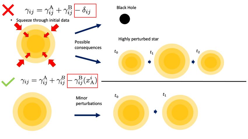
Figure 2. Graphical illustration of the spurious dynamics that may be introduced
by the simple superposition procedure (43). Upper panel: The spurious increase in
the volume element mimics a squeezing of the stellar core that effects a pulsation of
the star or may even trigger gravitational collapse to a BH. Lower panel: No such
squeezing occurs with the adjusted superposition (45), and the binary evolution
starts with approximately unperturbed stars.
course, precisely the contribution we subtract in the third term on the right-hand-side
and all would be well. In practice, however, the BSs start from initial positions xiA
and xiB with finite separation d = ||xiA − xiB || and we consequently perturb the metric
at star A’s centre by
B
δγij = γij (xiA ) − δij (44)
A i
away from its equilibrium value γij (xA ). This metric perturbation can be interpreted
√
as a distortion of the volume element γ at the centre of star A. More specifically,
the volume element at star A’s centre is enhanced by O(1) % for initial separations
O(100) M and likewise for the centre of star B (by symmetry); see appendix A of
Ref. [1] for more details.] The energy density ρ, on the other hand, is barely altered
by the presence of the other star, because of the exponential fall-off of the scalar field.
The leading-order error therefore consists in a small excess mass that has been added
to each BS’s central region. We graphically illustrate this effect in the upper half of
Fig. 2 together with some of the possible consequences. As we will see, this qualitative
interpretation is fully borne out by the phenomenology we observe in the binaries’ time
evolutions.
Finally, we would like to emphasise that, while evaluating the constraint violations
is in general a good rule of thumb to check whether the field configuration is a solution
of the system, it does not inform one whether it is the intended solution; a system with
some constraint violation may have drifted closer to a different, unintended solution. In
the present case, in addition to the increased constraint violation, the constructed BS
solutions possess significant excitations. Thus, while applying a constraint damping
√
] Due to the slow decay of this effect ∝ 1/ d [1], a simple cure in terms of using larger d is often
not practical.Malaise and remedy of binary boson-star initial data 14
system like conformal Z4 [92, 93] may eventually drive the system to a solution, it may
no longer be what was originally intended to be the initial condition of an unexcited
BS star.
3.2. Improved superposition
The problem of the simple superposition is encapsulated by Eq. (44) and the resulting
deviation of the volume elements at the stars’ centres away from their equilibrium
values. At the same time, the equation presents us with a concrete recipe to mitigate
this error: we merely need to replace in the simple superposition (43) the first relation
A B
γij = γij + γij − δij by
A B B
γij = γij + γij − γij (xiA ) = γij
A B
+ γij A i
− γij (xB ) . (45)
The two expressions on the right-hand side are indeed equal thanks to the symmetry
of our binary: its constituents have equal mass, no spin and their velocity components
i j i j
satisfy vA vA = vB vB for all i, j = 1, 2, 3 in the centre-of-mass frame. Equation
(45) manifestly ensures that at positions xiA and xiB we now recover the respective
star’s equilibrium metric and, hence, volume element. We graphically illustrate this
improvement in the bottom panel of Fig. 2.
A minor complication arises from the fact that the resulting spatial metric does
not asymptote towards δij as R → ∞. We accordingly impose outgoing Sommerfeld
A i
boundary conditions on the asymptotic background metric 2δij − γij (xB ); in a set of
test runs, however, we find this correction to result in very small changes well below
the simulation’s discretisation errors.
Finally, we note that the leading-order correction to the superposition as written
in Eq. (45) does not work for asymmetric configurations with unequal masses or spins.
Generalising the method to arbitrary binaries requires the subtraction of a spatially
B
varying term rather than a constant γij A i
(xiA ) = γij (xB ) or δij . Such a generalisation
A i B
may consist, for example, of a weighted sum of the terms γij (xB ) and γij (xiA ).
Leaving this generalisation for future work, we will focus on equal-mass systems in the
remainder of this study and explore the degree of improvement achieved with Eq. (45).
4. Models and results
For our analysis of the two types of superposed initial data, we will now discuss time
evolutions of binary BS head-on collisions. A head-on collision is characterised by
the two individual BS models and three further parameters, the initial separation in
units of the ADM mass, d/M , and the initial velocities vA and vB of the BSs. We
perform all our simulations in the centre-of-mass frame, so that for equal-mass binaries,
vA = −vB =.. v. One additional parameter arises from the type of superposition used
for the initial data construction: we either use the “plain” superposition of Eq. (43) or
the “adjusted” method (45).
For all our simulations, we set v = 0.1; this value allows us to cover a wide range
of initial separations without the simulations becoming prohibitively long. The BS
binary configurations summarised in Table 2 then result in four sequences of head-
on collisions labelled mini, +mini, soli and +soli, depending in the nature of the
constituent BSs and the superposition method. For each sequence, we vary the BSs
initial separation d to estimate the dependence of the outcome on d. First, however,Malaise and remedy of binary boson-star initial data 15
Table 2. The four types of BS binary head-on collisions simulated in this study.
The individual BSs A and B are given either by the mini or solitonic model
of Table 1, and start with initial velocity v directed towards each other. The
initial data is constructed either by plain superposition (43) or by adjusting the
superposed data according to Eq. (45). For each type of binary, we perform five
collisions with initial separations d listed in the final column.
Label star A star B v initial data d/M
mini mini mini 0.1 plain 75.5, 101, 126, 151, 176
+mini mini mini 0.1 adjusted 75.5, 101, 126, 151, 176
soli soli soli 0.1 plain 16.7, 22.3, 27.9, 33.5, 39.1
+soli soli soli 0.1 adjusted 16.7, 22.3, 27.9, 33.5, 39.1
we test our interpretation of the improved superposition (45) by computing the level
of constraint violations in the initial data.
4.1. Initial constraint violations
As discussed in Sec. 3.1 and in Appendix A of Ref. [1], the main shortcoming of the
plain superposition procedure consists in the distortion of the volume element near
the individual BSs’ centres and the resulting perturbation of the mass-energy inside
the stars away from their equilibrium values. If this interpretation is correct, we would
expect this effect to manifest itself in an elevated level of violation of the Hamiltonian
constraint (19) which relates the energy density to the spacetime curvature. Put
the other way round, we would expect our improved method (45) to reduce the
Hamiltonian constraint violation. This is indeed the case as demonstrated in the upper
panels of Fig. 3 where we plot the Hamiltonian constraint violation of the initial data
along the collision axis for the configurations mini and +mini with d = 101 M and
the configurations soli and +soli with d = 22.3 M .
In the limit of zero boost velocity v = 0, this effect is even tractable through
an analytic calculation which confirms that the improved superposition (45) ensures
H = 0 at the BS’s centres in isotropic coordinate; see Appendix A for more details.
Our adjustment (45) also leads to a reduction of the momentum constraint
violations of the initial data, although the effect is less dramatic here. The bottom
panels of Fig. 3 display the momentum constraint Mx of Eq. (20) along the collision
axis normalised by the momentum density 8πjx ; we see a reduction by a factor of a
few over large parts of the BS interior for the modified data +mini and +soli.
The overall degree of initial constraint violations is rather small in all cases,
well below 0.1 % for our adjusted data. These data should therefore also provide a
significantly improved initial guess for a full constraint solving procedure. We leave
such an analysis for future work and in the remainder of the work explore the impact
of the adjustment (45) on the physical results obtained from the initial data’s time
evolutions.
4.2. Convergence and numerical uncertainties
In order to put any differences in the time evolutions into context, we need to
understand the uncertainties inherent to our numerical simulations. For this purpose,
we have studied the convergence of the GW radiation generated by the head-on
collisions of mini and solitonic BSs.Malaise and remedy of binary boson-star initial data 16
mini, d = 101 M soli, d = 22.3 M
+mini, d = 101 M +soli, d = 22.3 M
-1
1×10
-2
1×10
|H| / (16πρctr)
-3
1×10
-4
1×10
-5
1×10
-3
1×10
|Mx| / (8πjx,ctr)
-4
1×10
-5
1×10
-6
1×10
-7
1×10
0 20 40 60 80 0 5 10 15 20 25
x/M x/M
Figure 3. Upper row: The Hamiltonian constraint violation H – Eq. (19) –
normalised by the respective BS’s central energy density 16πρctr is plotted along
the collision axis of the binary configurations mini, +mini with d = 101 M (left)
and soli, +soli with d = 22.3 M (right). The degree of violations is substantially
reduced in the BS interior by using the improved superposition (45) for +mini
and +soli relative to their plain counterparts; the maxima of H have dropped by
over an order of magnitude in both cases. Bottom row: The same analysis for the
momentum constraint Mx normalised by the central BS’s momentum density
8πjx . Here the improvement is less dramatic, but still yields a reduction by a
factor of a few in the BS core.
Figure 4 displays the convergence of the radiated energy Erad as a function of time
for the +mini configuration with d = 101 M of Table 1 obtained for grid resolutions
h1 = M/6.35, h2 = M/9.53 and h3 = M/12.70 on the innermost refinement level
and corresponding grid spacings on the other levels. The functions Erad (t) and their
differences are shown in the bottom and top panel, respectively, of Fig. 4 together with
an amplification of the high-resolution differences by the factor Q2 = 2.86 for second-
order convergence. The observation of second-order convergence is compatible with
the second-order ingredients of the Lean code, prolongation in time and the outgoing
radiation boundary conditions. We believe that this dominance is mainly due to the
smooth behaviour of the BS centre as compared with the case of black holes [94]. By
using the second-order Richardson extrapolated result, we determine the discretisation
error of our energy estimates as 0.9 % for h3 which is the resolution employed for all
remaining mini BS collisions. We have performed the same convergence analysis for the
plain-superposition counterpart mini and for the dominant (`, m) = (2, 0) multipole of
the Newman-Penrose scalar of both configurations and obtained the same convergence
and very similar relative errors.
In Fig. 5, we show the same convergence analysis for the solitonic collision +soli
with d = 22.3 M and resolutions h1 = M/22.9, h2 = M/45.9, h3 = M/68.8. WeMalaise and remedy of binary boson-star initial data 17
-6
10
-7 |Erad,h - Erad,h | / M
10 1 2
|Erad,h - Erad,h | / M
∆Erad / M
-8 2 3
10
Q2 |Erad,h - Erad,h | / M
2 3
-9
10
-10
10
-11
10
-5
6×10
Erad / M
-5
-5
6×10 Erad,h / M
4×10 1
Erad,h / M
2
-5 Erad,h / M
-5
2×10 4×10 700 800 900
3
Erad,Rich / M
0
0 200 400 600 800
t/M
Figure 4. Convergence analysis for the GW energy extracted at Rex = 252 M
from the head-on collision +mini of Table 1 with d = 101 M . For the resolutions
h1 = M/6.35, h2 = M/9.53 and h3 = 12.70 (on the innermost refinement level),
we obtain convergence close to second order (upper panel). The numerical error,
obtained by comparing our results with the second-order Richardson extrapolated
values (bottom panel), is 0.9 % (1.6 %, 3.6 %) for our high (medium, coarse)
resolutions.
-5
10
-6
10
-7
10
∆Erad / M
-8
10
-9 |Erad,h - Erad,h | / M
10 1 2
-10 |Erad,h - Erad,h | / M
10 2 3
-11 Q2 |Erad,h - Erad,h | / M
10 2 3
-4
8×10
-4
6.35×10
-4
6×10
Erad / M
-4
-4 6.30×10
Erad,h / M
4×10 1
Erad,h / M
2
-4 -4 Erad,h / M
2×10 6.25×10
150 200 250 3
Erad,Rich / M
0
0 100 200
t/M
Figure 5. Convergence analysis as in Fig. 4 but for the configuration +soli
of Table 1 with d = 22.3 M and resolutions h1 = M/22.9, h2 = M/45.9 and
h3 = M/68.8. The numerical error, obtained by comparing our results with the
second-order Richardson extrapolated values (bottom panel), is 0.03 % (0.07 %,
0.6 %) for our high (medium, coarse) resolutions.
observe second-order convergence during merger and ringdown and slightly higher
convergence in the earlier infall phase. For the uncertainty estimate we conservatively
use the second-order Richardson extrapolated result and obtain a discretisation errorMalaise and remedy of binary boson-star initial data 18
of about 0.07 % for our medium resolution h2 which is the value we employ in our
solitonic production runs. Again, we have repeated this analysis for the plain soli
counterpart and the (2, 0) GW multipole observing the same order of convergence and
similar uncertainties. Our error estimate for the solitonic configurations is rather small
in comparison to the mini BS collisions and we cannot entirely rule out a fortuitous
cancellation of errors in our simulations. From this point on, we therefore use a
conservative discretisation error estimate of 1 % for all our BS simulations.
A second source of uncertainty in our results is due to the extraction of the GW
signal at finite radii rather than I + . We determine this error by extracting the signal
at multiple radii, fitting the resulting data by the series expansion f = f0 + f1 /r,
and comparing the result at our outermost extraction radius with the limit f0 . This
procedure results in errors in Erad ranging between 0.5 % and 3 %. With the upper
range, we arrive at a conservative total error budget for discretisation and extraction
of about 4 %. As a final test, we have repeated the mini and +mini collisions
for d = 101 M with the independent GRChombo code [95, 96] using the CCZ4
formulation [93] and obtain the same results within ≈ 1.5 %. Bearing in mind these
tests and a 4 % error budget, we next study the dynamics of the BS head-on collisions
with and without our adjustment of the initial data.
4.3. Radiated gravitational-wave energy
For our first test, we compute the total radiated GW energy for all our head-on
collisions focusing in particular on its dependence on the initial separation d of the BS
centres. In this estimate we exclude any spurious or “junk” radiation content of the
initial data by starting the integration at t = Rex + 40 M . Unless specified otherwise,
all our results are extracted at Rex = 300 M for mini BS collisions and Rex = 84 M
for the solitonic binaries.
The main effect of increasing the initial separation is a reduction of the (negative)
binding energy of the binary and a corresponding increase of the collision velocity
around merger. In the large d limit, however, this effect becomes negligible. For the
comparatively large initial separations chosen in our collisions, we would therefore
expect the function Erad to be approximately constant, possibly showing a mild
increase with d. The mini BS collisions shown as black × symbols in the upper panel
of Fig. 6 exhibit a rather different behaviour: the radiated energy rapidly decreases
with d and only levels off for d & 150 M . We have verified that the excess energy
for smaller d is not due to an elevated level of junk radiation which consistently
contribute well below 0.1 % of Erad in all our mini BS collisions and has been excluded
from the results of Fig. 6 anyway. The +mini BS collisions, in contrast, results in an
approximately constant Erad with a total variation approximately at the level of the
numerical uncertainties. For d & 150 M , both types of initial data yield compatible
results, as is expected. The key benefit of our adjusted initial data is that they provide
reliable results even for smaller initial separations suitable for starting BS inspirals.
The discrepancy is less pronounced for the head-on collisions of solitonic BS
collisions; both types of initial data result in approximately constant Erad . They differ,
however, in the predicted amount of radiation at a level that is significant compared
to the numerical uncertainties. As we will see below, this difference is accompanied by
drastic differences in the BS’s dynamics during the long infall period. We furthermore
note that the mild but steady increase obtained for the adjusted +soli agrees better
with the physical expectations.Malaise and remedy of binary boson-star initial data 19
Erad / M
-4
1×10 mini
+mini
-5
9×10
-5
8×10
-5
7×10
-5
6×10 80 100 120 140 180 200
160
d /M
Erad / M
-4
soli
7.5×10 +soli
-4
7.0×10
-4
6.5×10
-4
6.0×10
-4
5.5×10 10 20 30 40
15 25 35
d/M
Figure 6. The GW energy Erad generated in the head-on collision of mini (upper
panel) and solitonic (lower panel) BS binaries starting with initial separation d
and velocity v = 0.1 towards each other. For comparison, a non-spinning, equal-
mass BH binary colliding head-on with the same boost velocity v = 0.1 radiates
Erad = 6.0 × 10⁻⁴ M [89].
The differences in the total radiated GW energy also manifest themselves in
different amplitudes of the (2, 0) multipole of the Newman-Penrose scalar Ψ4 . This is
displayed in Figs. 7 and 8 where we show the GW modes for the mini and solitonic
collisions, respectively. The most prominent difference between the results for plain
and adjusted initial data is the significant variation of the amplitude of the (2, 0) mode
in the plain mini BS collisions in the upper panel of Fig. 7. In contrast, the differences
in the amplitudes in Fig. 8 for the solitonic collisions are very small. In fact, the
differences in the radiated energy of the soli and +soli collisions mostly arise from
a minor stretching of the signal for the soli case; this effect is barely perceptible
in Fig. 8 but is amplified by the integration in time when we calculate the energy.
Finally, we note the different times of arrival of the main pulses in Fig. 8; especially
for larger initial separation, the merger occurs earlier for the soli configurations than
for their adjusted counterparts +soli. We will discuss this effect together with the
evolution of the scalar field amplitude in the next subsection.
4.4. Evolution of the scalar amplitude and gravitational collapse
The adjustment (45) in the superposition of oscillatons was originally developed in
Ref. [1] to reduce spurious modulations in the scalar field amplitude; cf. their Fig. 7.
In our simulations, this effect manifests itself most dramatically in the collisions of
our solitonic BS configurations soli and +soli. From Fig. 1, we recall that the
single-BS constituents of these binaries are stable, but highly compact stars, located
fairly close to the instability threshold. We would therefore expect them to be more
sensitive to spurious modulations in their central energy density. This is exactly
what we observe in all time evolutions of the soli configurations starting with plain-
superposition initial data. As one example, we show in Fig. 9 the scalar amplitude atMalaise and remedy of binary boson-star initial data 20
0.0004
0.0002
0
MR ψ20
-0.0002 mini, d=75.5
-0.0004 mini, d=101
mini, d=126
-0.0006 mini, d=151
mini, d=176
-0.0008
0.0004
0.0002
0
MR ψ20
-0.0002 +mini, d=75.5
-0.0004 +mini, d=101
+mini, d=126
-0.0006 +mini, d=151
+mini, d=176
-0.0008
0 200 400 600 800 1000
t/M
Figure 7. The (2, 0) mode of the Newman-Penrose scalar for the mini boson star
collisions of Table 1.
0.01
MR ψ20
0
soli, d=16.7 M
soli, d=22.3 M
-0.01 soli, d=27.9 M
soli, d=33.5 M
soli, d=39.1 M
-0.02
0.01
MR ψ20
0
+soli, d=16.7 M
+soli, d=22.3 M
-0.01 +soli, d=27.9 M
+soli, d=33.5 M
+soli, d=39.1 M
-0.02
0 50 100 150 200
t/M
Figure 8. The (2, 0) mode of the Newman-Penrose scalar for the solitonic boson
star collisions of Table 1.
the individual BS centres and the BS trajectories as functions of time for the soli and
+soli configurations starting with initial separation d = 22.3 M . Let us first consider
the soli configuration using plain superposition displayed by the solid (black) curves.
In the upper panel of Fig. 9, we clearly see that the scalar amplitude steadily increases,
reaching a maximum around t ≈ 30 M and then rapidly drops to a near-zero level.
Our interpretation of this behaviour as a collapse to a BH is confirmed by the horizon
finder which reports an apparent horizon of irreducible mass mirr = 0.5 M just before
the scalar field amplitude collapses; the time of the first identification of an apparent
horizon is marked by the vertical dotted black line at t ≈ 30 M . For reference we
plot in the bottom panel the trajectory of the BS centres along their collision (hereMalaise and remedy of binary boson-star initial data 21
soli, d=22.3 M
0.25 +soli, d=22.3 M
single BS
0.2 single BS, poisoned
|ϕctr|
0.15
0.1
0.05
0
10
5
x/M
0
-5
-10
0 20 40 60 80 100
t/M
Figure 9. The central scalar-field amplitude |ϕctr | as a function of time for one
BS in the head-on collisions of solitonic BSs with distance d = 22.3 M (black solid
and red long-dashed) as well as a single BS spacetime with the same parameters
(green dashed) and the same single BS spacetime “poisoned” with the metric
perturbation (44) that would arise in a simple superposition (see text for details).
The dotted vertical lines mark the first location of an apparent horizon in the
simulation of the same colour; as expected, no horizon ever forms in the evolution
of the unpoisoned single BS. In the bottom panel, we show for reference the
coordinate trajectories of the BS centres as obtained from locally Gauss-fitting
the scalar profile. Around merger this procedure becomes inaccurate, so that the
values around t ≈ 70 M should be regarded as qualitative measures, only.
the x) axis. In agreement with the horizon mass mirr = 0.5 M , the trajectory clearly
indicates that around t ≈ 30 M , the BSs are still far away from merging into a single
BH; in units of the ADM mass, the individual BS radius is r99 = 2.78 M . We interpret
this early BH collapse as a spurious feature due to the use of plain superposition in
the initial data construction. This behaviour is also seen in the case of the real scalar
field oscillatons in [1].
We have tested this hypothesis with the evolution of the adjusted initial data.
These exhibit a drastically different behaviour in the collision +soli displayed by
the dashed (red) curves in Fig. 9. Throughout most of the infall, the central scalar
amplitude is constant, it increases mildly when the BS trajectories meet near x = 0,
and then rapidly drops to zero. Just as the maximum amplitude is reached, the horizon
finder first computes an apparent horizon, now with mirr = 0.99 M , as expected for a
BH resulting from the merger; see the vertical red line in the figure.
As a final test of our interpretation, we compare the behaviour of the binary
constituents with that of single BSs boosted with the same velocity v = 0.1. As
expected, the scalar field amplitude at the centre of such a single BS remains constant
within high precision, about O(10−5 ), on the timescale of our collisions. We have then
repeated the single BS evolution by poisoning the initial data with the very same term
(44) that is also added near a single BS’s centre by the plain-superposition procedure.
The resulting scalar amplitude at the centre of this poisoned BS is shown as the
dash-dotted (blue) curve in Fig. 9 and nearly overlaps with the corresponding curveYou can also read