TRADING VOLATILITY TRADING STRATEGIES BASED ON THE VIX TERM STRUCTURE - OSKAR FRANSSON, HENRIK MARK ALMQVIST - DIVA
←
→
Page content transcription
If your browser does not render page correctly, please read the page content below

Trading volatility
Trading strategies based on the VIX term
                structure
          Oskar Fransson, Henrik Mark Almqvist

            Department of Business Administration
               International Business Program
           Bachelor Thesis, 15 Credits, Spring 2020
                 Supervisor: Irina Alexeyeva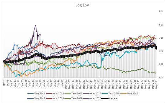
Page intentionally left blank
Acknowledgement

We would like to thank our supervisor Irina Alexeyeva for her support and feedback
throughout the process of writing this thesis.

Umeå University, May 2020

Henrik Mark-Almqvist
Oskar Fransson

Page intentionally left blank
Abstract
This study investigates how term structure dynamics of VIX futures can be exploited for
abnormal returns. To be able to access volatility as a tradeable asset, the trading strategies
only trades ETFs which are designed to replicate the movements of VIX futures index. It
is established that such ETFs are unsuitable for buy-and-hold investments because of the
negative roll yield it usually suffers, caused by the slope of the VIX term structure.
Consequently, these conditions create opportunities for strategies that use direct and
inverse VIX ETFs to be profitable. The study is a quantitative study that uses historical
price data to back test three different trading strategies. The strategies are tested over the
period 11-oct-2011 to 31-mar-2020. The authors have deliberately chosen to delimit the
study by not testing the performance of the ETFs, not statistically test the risk-adjusted
returns and not perform a regression to calculate optimal hedge ratios for the strategies.
The results from this study shows that its possible for strategies that exploit the term
structure dynamics of VIX futures to generate abnormal returns.
Page intentionally left blank
Table of content
1. Introduction                                      1
  1.1 Background                                     1
  1.2 Problematization                               2
    Figure 1.                                        2
  1.3 Research Question                              3
  1.4 Purpose                                        3
  1.5 Contribution                                   4
  1.6 Delimitations                                  4
2. Theoretical Background                            6
  2.1 The Dynamics of Volatility in Equity Markets   6
    Figure 2.                                        7
  2.2 The VIX-index                                  7
  2.3 VIX Term Structure                             8
    Figure 3.                                        8
  2.4 Long VIX Futures, a Poor Trade                 9
    Figure 4                                         9
  2.5 Rational Expectation Theory                    10
  2.6 Efficient Market Hypothesis                    11
  2.7 Trading based on the VIX term structure        11
3. Methodology                                       13
  3.1 Research philosophy                            13
  3.2 Ontology                                       13
  3.3 Epistemology                                   13
  3.4 Research strategy and methodological choice    14
  3.5 Research Approach                              14
  3.6 Research Design                                15
  3.7 Literature search and source criticism         15
    Figure 5.                                        16
  3.8 Ethical and societal considerations            16
4. Research Methods                                  17
  4.1 Data                                           17
    Figure 6.                                        18
  4.2 The Trading Strategies                         18
Figure 7. 20
Figure 8. 21
Figure 9. 22
4.3 Performance Measurements 22
4.4 Abnormal Returns 24
4.5 Empirical Tests 24
4.6 Bootstrapping 26
5. Results 27
5.1 Strategy Performance 27
Table 1. 27
Figure 10. 28
Figure 11. 29
Figure 12. 30
Figure 13. 30
5.2 Descriptive Statistics 30
Table 2. 31
Table 3. 31
5.3 Normality Tests 32
Table 4 32
Table 5 32
Table 6 33
Table 7 33
5.4 Two sample T-test 33
Table 8 34
Table 9 34
5.5 Quality Criteria 34
5.5.1 Reliability 34
5.5.2 Validity 35
5.5.3 Generalizability and replicability 35
6. Analysis and Discussion 36
6.1 The LSV Strategy 36
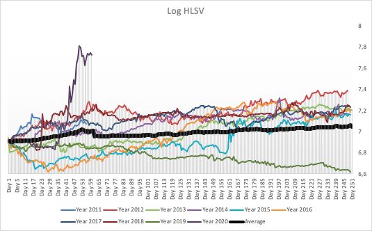
6.2 The HLSV Strategy 37
6.3 The LSLV Strategy 37
6.4 Empirical Tests 37
6.5 Theoretical Implications 387. Conclusion 39 7.1 Summary 39 7.2 Future research 40 7.3 Limitations 40 Reference List 41
1. Introduction
In the introduction the authors present the background behind the idea of the research,
previous relevant studies, following with a problematization leading to the research
purpose. Finally, the contribution of the research and some delimitations are disclosed.

1.1 Background

In the field of finance and in particular portfolio management, the balance between risk
and return aims to be optimized. An assets return is the percentage change between two
periods prices and the assets risk is traditionally defined as the standard deviation (or
volatility) over the periods return, which explains the extent of fluctuations for an asset’s
historical prices (Berk & DeMarzo, 2014, p. 323). This research investigates how
volatility can be traded as an asset, the unique features of volatility instruments and how
it can be used for profitable strategies.

In 1993, Professor Robert Whaley created the Cboe VIX-index, which prices are designed
to represent the S&P 500 30 days expected future volatility (Chicago Board Options
Exchange [CBOE], 2019). The reason for why the VIX index will be emphasized
repeatedly in the essay is because it is important to understand how it is derived, how it
relates to the stock market and how investors uses it in their forecasts and predictions.
The VIX index and its spot prices itself is not a tradeable asset because the prices are only
derived from a basket of S&P 500 underlying index options. However, since 2004 the
Chicago board of option exchange (Cboe) launched VIX futures contracts of the VIX spot
prices. Since VIX futures inception, volatility as an asset have gotten more attention
among traders and scholars, and there’s been a large increase in tradable products for VIX
as an underlying instrument. The VIX index has been proven to generate returns with a
negative correlation to the stock market, which has led to an alternative way for investors
to hedge their equity portfolio if one does not want to use derivatives linked directly to
the stock market (Cboe, 2019).

Several existing literatures that analyzes the pricing of VIX derivatives have investigated
the behavior of the VIX term structure and to what extent established economic theories
can explain the dynamics of it. Most of the research conclude that the economic theory
of rational expectation fails to explain the dynamics of VIX futures and the VIX index
price (Nossman & Wilhelmsson, 2009; Simon & Campassano, 2012). The argument
behind this is based on the fact that investors are willing to pay considerable amounts to
hedge their equity portfolios. In the pricing of VIX derivatives this cost is referred to as
VIX risk premium. From an economic point of view this premium could be interpreted
as the expected return of selling a VIX future contract. Since there is a high demand on
this kind of insurance among investors, the premiums may differ substantially between
the VIX futures and the VIX index spot level (Alkelin & Bergkvist, 2019, p. 2). The
outcome of this fact is that the VIX term structure often is upward sloping (Alexander,
Kapraun & Korovilas, 2015, p.315). Thereupon, this dynamic has given rise to several
trading strategies using the term structure of the VIX futures for capitalization.

                                             1
1.2 Problematization
Because of the inverse relationship between volatility and equity prices and the mean
reverting dynamics of VIX (figure 1), VIX futures can be expected to give a potential
interesting hedging opportunity for an equity portfolio (Jung, 2016, p.190).
Figure 1.
Figure 1. VIX index and S&P 500: Black - SPY, Blue - VIX index.
Source: Reuters Eikon (2020).
However, professor Whaley (2013) shows that a long-term holding position of VIX
futures is a poor buy-and-hold strategy and generates negative return over time because
the futures normally trades with negative carry and roll yield. The long VIX future
position suffers from negative roll yield of the degree to which VIX spot prices and VIX
futures prices relate to each other (Whaley, 2013, p.12-13). Previous literature by Asensio
(2013) describes how there is an imbalance between the VIX index and prices of VIX
futures, creating a slope of the VIX term structure (contango and backwardation). This
could be explained with the market consistently expecting higher (contango) or lower
(backwardation) prices of the future VIX spot prices (Asensio, 2013, p.2). Furthermore,
Simon and Campassano (2012) describes how these imbalances on the term structure
have an insignificant forecast power for the VIX index prices, implying there’s is a time-
varying risk premium (Simon & Campassano, 2012, p.2). Additional studies by Simon
and Campassano (2012) and Bordonado and Samdal (2016) shows that trading strategies
based on the slope of the VIX term structure can be profitable by taking position
capitalizing on the roll yield.
2During the last decade, there has been a significant increase of traded volume in VIX
exchange traded funds (ETFs). An ETF is a variation of an exchange traded product
(ETP) that can expand the opportunities to trade volatility without having to directly use
financial derivatives as options or futures. An ETF is best explained as a collection of
various financial instruments that are bundled together for the purpose of following a
specific underlying asset, such as the VIX- index. This thesis will be focusing on various
ETFs with VIX futures as underlying. Products such as ETFs, which are designed to
follow the volatility futures movement, are therefore also affected by similar term
structure characteristics (Bordonado & Samdal, 2016, p.35). Since a term structure in
contango suffers from negative roll yield and carry, it causes a passive buy-and-hold
investment in VIX ETFs to be less suitable if one wants to maximize profit over time
(Whaley, 2013, p19). Further research by Bordonado and Samdal (2016) show how
similar trading strategies as presented by Simon and Campassano (2012) can be applied
for trading VIX ETPs/ETFs.
Trading strategies shorting equity volatility are exposed to the risk of volatility spikes.
This means that an investor must not only avoid losing due to the slope of the term
structure, but also for more unexpected tail events that can greatly increase volatility. For
instance, February 5th, 2018 was the day when the VIX index experienced its largest
daily increase since the index inception, an event also referred to as “Volmageddon”.
Volmageddon had a catastrophic impact especially on short VIX short term ETFs, which
for example forced the “VelocityShares daily inverse VIX short term note ETF” to be
liquidated (Kawa, 2019). This day has since its occurrence symbolized the cannibalized
returns and tail-events associated with these kinds of trading strategies. The question that
arises is how portfolios can be managed to avoid the negative effects of this kind of
events.
1.3 Research Question
The thesis aims to answer the following research question:
“How can the term structure dynamics of VIX futures be exploited for abnormal
returns?”
1.4 Purpose
The purpose with this paper is to investigate if trading strategies that exploits VIX term
structure behavior (similar to strategies done by Simon and Campassano (2012)) have
generated a significant abnormal return during the latest 7 years. The time period used in
this study exceeds the periods tested in previous literature, which include significant
volatile events that could have an effect on short volatility strategies. This makes it is
interesting to investigate the question regarding the robustness of the strategies.
Furthermore, the thesis will investigate whether different modifications of the strategies
have generated significant abnormal returns and how similar trading inputs can be useful
to protect equity portfolios.
3The intention with this research is to provide more insight into how a discrepancy in the
markets can be used to profit from by exploiting the dynamics of VIX derivatives.
Further, this thesis is expected to increase the understanding of how trading strategies can
be applied and highlight the involved financial risks.
1.5 Contribution
This thesis aims to investigate if trading strategies that exploit VIX term structure
behavior has generated abnormal returns during the latest 7 years. By improving the
knowledge about this topic of research the authors hope to provide empirical foundation
and new perspectives to previous research as this study examines a time period not yet
investigated. The time period that this study covers contains interesting events that could
have a remarkable effect on the performance on trading strategies trying to profit by
utilizing the term structure of VIX futures.
The results from the study could also contribute to further theoretical implications. The
rational expectation theory is criticized in this study as the authors see that it fails to
explain the price development of VIX index. If the trading strategies tested in this study
should generate abnormal returns compared to the benchmark it would mean that the term
structure can be exploited as predictor for VIX futures return. If this is the case the study
aligns with the results of similar research and contribute with further evidence that the
rational expectation theory cannot explain this phenomenon.
Furthermore, theories regarding efficient markets will as well be applied as theoretical
implication. The efficient market hypothesis is a debatable subject in the field of finance
and is closely related to the theories of rational expectation, stating that market returns is
not predictable. Hence the performed hypothesis testing in this research could further
contribute in the debate of efficient markets.
The contribution of this study can be relevant for traders and investors that seek to get
more knowledge about the dynamics of the VIX index and exchange traded products
related to it. Based on the results, the strategies themselves could be an attractive way for
people to manage their savings. But most important that the results of the trading
strategies could create a clearer picture why and how actively a portfolio dealing with
these products must be managed. The practical contribution of the study will therefore be
connected to the decision-making progress made by traders and investors that are
interested to use these kinds of products.
1.6 Delimitations
To be able to conduct a viable thesis some delimitation will be presented. First off, the
strategies presented is solely back tested using products categorized as exchange traded
funds. The question of the thesis may seem a bit broad to be answered as one could go
deeper into how other products could open up alternative opportunities to generate
abnormal returns. Since the purpose of the study is to test strategies similar to other
studies but during a different time period, tests of the ETFs abilities on tracking their
underlying asset might be taken into consideration. This type of statistical testing is
performed in previous studies but given that the purpose of the study is not to measure
4the performance of the products but rather how it can be used to generate abnormal
returns, this will not be investigated. Another delimitation is that no empirical tests will
be done on the risk adjusted returns which can affect the credibility of the results. In
previous research from Simon and Campassano (2012), they documented how regression
test could be performed with the purpose to determine the best hedge ratio for strategies
trading VIX futures. The authors in this paper will not perform statistical testing to
determine a hedge ratio, but only assume a 0,5-hedge ratio for the back-testing period.
1.7 Disposition
Introduction
In the introduction the authors present the background behind the idea of the research,
previous relevant studies, following with a problematization leading to the research
purpose. Finally, the contribution of the research and some delimitations are disclosed.
Theoretical Background
In the theoretical background, essential theories and facts of the thesis are presented. In
the latter part, a couple of established financial theories is lifted with the purpose to
discuss how the practical implications of those can be connected with the final results.
Methodology
The methodology explains the philosophical and theoretical approaches applied in the
research and its overall design. Further, approaches regarding the process of literature
search can be read. In the final part of the chapter the considerations on ethics and societal
aspects are stated.
Research methods
This chapter presents how the process of the quantitative study is performed, how the data
is collected and how the strategy is created. Further, the authors present the related
hypothesis as well as measurements tools, statistics and empirical tests applied in this
study.
Results
This chapter includes the presentation and explanation of statistics and performance
measurement. In the following part, the empirical tests of the hypothesis and a disclosure
of quality criteria is presented.
Analysis and discussion
This chapter includes interpretation, discussion and analysis of the results presented in
the previous chapter. It aims to connect theories and arguments with the empirical
findings to answer the study research question.
Conclusion
The last chapter will include a summary of the study where the authors reflect upon the
findings, the limitations and suggestions for future studies.
52. Theoretical Background
In the theoretical background, essential theories and facts of the thesis are presented. In
the latter part, a couple of established financial theories is lifted with the purpose to
discuss how the practical implications of those can be connected with the final results.
2.1 The Dynamics of Volatility in Equity Markets
As mentioned earlier, the historical volatility is calculated as the standard deviation
(square root of variance ! ! ) on a set of historical prices.
#
1
! ! = &((" − (̅ )!
$
"$%
Where n is the sample size, (" is the , &' return and (̅ is the mean return (Sinclair, 2013 p.
14). Since Black, Scholes and Merton introduced their option-pricing formula, its
fundamentals have been essential for modelling options. The formula is calculated based
on 7 parameters: current time -, current stock price ., option exercise /, strike 0, interest
rate 1, dividend rate γ, and volatility θ. Since all parameters but volatility θ is directly
observable in the financial markets, the volatility can be estimated by backing the Black-
Scholes formula (also referred as implied volatility), which can be explained as the market
expectations of future volatility at a given strike (Andersen & Brotherton-Ratcliffe, 1997,
p.5).
The difference of implied volatility between at-the-money (ATM) options and out/in-the-
money (O/ITM) options is traditionally referred to as the volatility-skew. Since the Black-
Scholes formula is based on the assumption that stock prices follow a normal distribution
of returns (Macroption, 2020), the Black-Scholes model also assume that the implied
volatility should be the same across the strike dimension (Ann, 2019). However, studies
by Foresi and Wu (2005) proves how OTM call and put options on equity indices, on
average exhibits implied volatilities with heavily skewed pattern. A structure where OTM
put options tend to be priced with higher implied volatility than OTM call options, a
pattern referred as volatility “smirk” (figure 2). Thus, causing OTM put options more
expensive than the corresponding OTM call option, implying that the risk-neutral
distribution for equity indexes are heavily skewed to the downside (Wu & Foresi, 2005,
p.9). Hence, this pricing nature of volatility in equity options corresponds with the inverse
relationship between S&P 500 and the VIX index.
6Figure 2.
Figure 2. The volatility Skew, “Smirk”: Blue line - implied volatility on OTM strikes of
S&P 500 options.
Source: CME QuikStrike (2020)
Foresi and Wu (2005) prove that the negative skew on implied volatility over the strike
dimension is a natural state for global equity index options. There are however many
possible explanations why this asymmetry exists. One explanation is that big jumps in
spot prices tend to be down, rather than up. An unexpected significant change in share
prices usually occur to the downside since the bad event is usually more unexpected,
compared with when good events occur, which usually is less unexpected (Bennett, 2014,
p. 187-188). Another explanation is that volatility is a measure of risk and leverage, and
leverage increases as equities declines. In a scenario where a company’s share price
declines (assuming no additional issue in shares or amount of debt) the company's
debt/equity ratio increases, hence the company’s leverage increase. Therefore, as
volatility and leverage are measures of risk, there is a correlation between leverage and
volatility as equities decreases (Bennett, 2014, p.187-188).
2.2 The VIX-index
The Cboe VIX-index was first introduced in 1993 with the intentions to measure the
market's expectation of 30-day volatility, implied by at-the-money S&P 100 index option
prices. Even though the VIX-index has evolved through time, the index became an
accepted benchmark for the stock market in United States soon after introduction. The
index is often mentioned in financial publications where it usually is more dramatically
referred to as the fear gauge (Cboe, 2019).
As mentioned, the Cboe VIX -index has developed during its lifetime. Ten year after
Cboe first introduced the index, it was updated with a new way to measure expected
volatility which is still actively used in the financial sector. The updated version of the
VIX index is based on the S&P 500 Index (SPX), a body for U.S. Equities. The new
mechanics of the index became to estimate the expected volatility by aggregating the
weighted prices of S&P 500 put and call options for a broad range of exercise prices. In
2014, VIX was upgraded again by including series of S&P 500 options with weekly
expiration periods (SPX Weeklies). The SPX weeklies are useful to provide an index that
7more precisely follow the 30-day target timeframe that the VIX intends to represent
(Cboe, 2019).
As the volatility has a strong negative correlation to stock market returns, an opportunity
arises to include volatility in an investment portfolio for its diversification properties. In
March 2004 Cboe launched the first exchange traded product, the VIX future contract,
with the reason of making it more accessible to trade volatility as an asset. Two years
later, in 2006, Cboe took it one step further and introduced VIX -options which
immediately grew to the most popular new product in Cboe’s history. Today, there are
several different exchange traded products to use in addition to derivatives as futures and
options, such as exchange traded notes and exchange traded fund (Cboe, 2019).
2.3 VIX Term Structure
Just like government bond yields or commodities futures usually is compared over
different maturities as a term structure (or yield curve), same can be done with different
maturities of VIX futures prices, creating a term structure on all futures maturities (and
the spot price). There are two key dynamics of the term structure: contango and
backwardation. In contango the longer dated maturities of VIX futures are more
expensive than the shorter-term futures and the spot price, illustrating upward sloping
curve in figure 3. Most of the time the VIX futures are in contango, but in times of
increased risk and volatility in the equity markets VIX futures are usually in
backwardation, structured with lower priced long term VIX future price compared to spot
price and shorter-term maturities (Bennett, 2014, p.185).
Figure 3.
Figure 3. VIX term structure: Blue line - contango, Green line - backwardation.
Source: VIX central (2020).
82.4 Long VIX Futures, a Poor Trade
The different dynamics of the VIX term structure problematize a long term buy and hold
position in VIX futures, since a VIX future term structure in contango is characterized
with a negative carry and roll yield which causes the position to generate negative return
over time (Whaley, 2013, p.12-13).
Previous literature where buy-and-hold strategies for VIX ETPs have been evaluated,
most have documented that the ETPs is also not a sustainable strategy for investing
(illustrated in figure 4). The conclusion drawn is that the investors who lose by taking
passive positions on these products have too little knowledge of the product’s structure
and nature, or act irrationally on the given information (Whaley, 2013, p.18). Various
studies have also shown that the buy-and-hold strategy performs worst if one uses ETPs
with benchmark to follow VIX short-term future indexes (Whaley, 2013, p.19). The ETPs
show particularly poor returns when the term structure is in contango but better returns
when the market is in backwardation. It therefore becomes clearer that the return is
negatively affected by taking a long position as the market is more often in contango and
backwardation happens more seldom (Bennett, 2014, p.184). This creates a demand for
more sophisticated trading strategies that can reduce the negative effects of the contango
trap. To lead the discussion back to the question of this paper, how the VIX term structure
could be utilized to generate abnormal returns, interesting questions arises regarding how
the roll yield can be captured in a trading strategy.
Figure 4
Figure 4. VIX short term ETFs and ETNs
Source: Reuters Eikon (2020)
92.5 Rational Expectation Theory
The rational expectation theory is an economic theory developed by John Muth in 1961,
often applied on research analyzing the term structure of interest rates (Deley & Sergi,
2019, p.5). The theory states that expectations will be identical to the optimal forecast
using all available information. An important fact to point out with rational expectations
is that even though the optimal forecast is based on all available information, a prediction
constructed from the forecast does not necessarily need to be perfectly accurate. This
theory was developed as a reaction to the objections of previous theories that tried to
explain the formation of expectation based from past experience only (Madura, 2014,
p.135).
Two reasons why an expectation fail to be rational would be that people might be unaware
of information that would have an effect on the future outcome and/or that people are
aware of all information but do not want to make the effort to make their expectation the
best guess of the future. To avoid confusion, it is also worth mentioning that if important
information that could have an effect on the outcome is unavailable the prediction may
fail to be accurate but the expectation would still be considered rational as it takes account
to all information available (Madura, 2014, p.136).
Applying this theory to the prices of VIX futures it suggests that the prices of the VIX
futures are unbiased predictors of the future VIX index spot prices. The slope of the VIX
term structure should therefore forecast the progress of the VIX spot index itself
(Bordonado & Samdal, 2016, p.21). However, research by Nossman and Wilhelmsson
(2009) proves how the expectation hypothesis on VIX futures can strongly be rejected
and that VIX futures prices constantly overestimates realized volatility (VIX spot)
(Nossman and Wilhelmsson, 2009, p.65). The research by Campassano and Simon (2012)
further confirms this rejection of the rational expectation hypothesis. They present
evidence that the term structure can be used as a predictor for the VIX futures. That is, if
the VIX futures trades above the VIX spot, the futures tend to fall, and if the futures trades
below the spot, the futures tend to raise. The rational expectation hypothesis should
contradict this evidence. Stating that future prices is an unbiased predictor of the future
value of spot (VIX spot should progress according to the slope of the term structure), and
if this was true the basis would not have predictive power (Sinclair, 2013, p.225).
Furthermore, according to Simon and Campassano (2012), the characteristics of the term
structure suggests that longer dated expiration of VIX futures discounts for a risk premia,
and that VIX futures prices tend to roll down during contango and roll up during
backwardation, causing a negative (positive) carry of term premia in contango
(backwardation). The evidence can explain the historically poor performance of long VIX
futures positions (Campassano & Simon, 2012, p.21)
The term structure itself could be explained by the fact that investors are risk averse and
that they are likely to pay a premium for VIX exposure. This premium could represent an
insurance against losses in the equity market. Additionally, Nossman and Wilhelmsson
(2009) presents evidence that the hypothesis cannot longer be rejected if the VIX futures
prices is adjusted for a risk premium. In fact, Nossman and Wilhelmsson presents
evidence indicating that VIX futures prices, when adjusted for risk premium to be a good
predictor of the VIX index spot prices (Nossman and Wilhelmsson, 2009, p.65).
102.6 Efficient Market Hypothesis
In 1970, Eugene Fama introduced the hypothesis of efficient market which states that
prices of financial assets, at some point, fully reflect all available information. This
hypothesis points out that prices trades at an equilibrium which is an effect of every
market participant having the same available information. The price equilibrium only
moves on new available information which per definition is an unpredicted event.
Therefore, prices in capital markets is unpredictable and abnormal return shouldn't be
possible. This leads to the essential argument of the efficient market hypothesis, that
prices in financial markets follows a random walk (Bodie, Kane & Marcus, 2014, p.351-
352).
In Famas work on efficient markets in 1970, he further introduces three versions of the
hypothesis, which represents versions of the theory in context with what type of
information is considered: weak-form, semi strong-form and strong-form. The weak form
suggests that all historic information that can be derived from market data (such as
historical prices and trading volume) is reflected in the market price. Hence, strategies
based on historical market data that is reliable for predicting prices should already be
known and exploited between all market participants. Consequently, the strategy loses its
predictive value since prices trades immediately at its fair value and the strategy will no
longer be able to predict future price changes. The semi strong-form states that all
information available in the market is reflected in prices. That is, in addition to historic
market data, all fundamental information as well, such as balance sheet, patents held,
earning forecasts and management. The strong form of efficient market hypothesis states
that all form of information is reflected in prices, including information not available to
the public, this version of the hypothesis suggests that insider trading is a reflection of
price equilibrium. (Bodie, Kane & Marcus, 2014, p.353-354)
According to Bodie, Kane and Marcus (2014), the efficient market hypothesis is a highly
debatable subject in the academic and industry of finance. Even though the efficient
market hypothesis is a widely accepted subject among scholars, there is still several
studies rejecting it. Examples of such studies that provide proofs of variables being able
to predict market returns have been documented by Fama and French in 1988, concluding
that higher dividend yield ratio can predict higher market return. Furthermore, a study by
Campbell and Shiller shows how earning yields as well can predict market returns. A
study done by Keim and Stambaugh proved that yield spreads between high- and low
grades corporate bonds could predict stock market returns (Bodie, Kane & Marcus, 2014,
p.365-366). Yet, the contradictory argument is that the interpretation of these results is
difficult, and the results is not an indication of a capturing of abnormal risk-adjusted
return, but rather an prediction of risk premium, hence the hypothesis of efficient markets
cannot be rejected (Bodie, Kane & Marcus, 2014, p.362-366).
2.7 Trading based on the VIX term structure
Campassano and Simon (2012) introduced a trading strategy with the purpose to
capitalize based on the fact that the rational expectation hypothesis can be strongly
rejected on VIX futures. This was done by trading VIX futures, aiming to capitalize on
the up and down roll of VIX futures positions. The trading strategy involves shorting the
11front month future contract when the VIX term structure is in contango and buying the
future contract when the term structure is in backwardation. Both of these positions are
exposed for unfavorable movements of the VIX futures prices; thus, this risk is hedged
by taking position of S&P futures. A short position in VIX futures are matched with
shorting S&P futures and long VIX futures are matched with long S&P futures. This
hedging technique is based on the tendency that VIX future prices and S&P futures
returns move inversely and thereupon the capitalization is essentially a collection of roll
yield. Additionally, Bordonado and Samdal (2016) presents evidence that VIX ETP
follow VIX future indices quite well and proved that approaches of adopting similar
strategies as Campassano and Simon (2012) could be done for trading VIX ETFs.
123. Methodology
The methodology explains the philosophical and theoretical approaches applied in the
research and its overall design. Further, approaches regarding the process of literature
search can be read. In the final part of the chapter the considerations on ethics and
societal aspects are stated.
3.1 Research philosophy
When defining the term research philosophy, it refers to different beliefs and assumptions
regarding the development of knowledge. Throughout a study the author will make
different types of assumptions, consciously or not. These assumptions include how the
authors perceive human knowledge (epistemology), and reality (ontology). These
assumptions will have an impact on how the authors shape the research, thus create a
deeper understanding of how to approach the research question, what method to use and
how to interpret the results (Saunders, 2009, p.124).
3.2 Ontology
Ontology is the knowledge regarding existence and relates to the nature of reality, thus
what exists and how one perceives it (Burrell and Morgan, 1979, cited in Holden &
Lynch, 2004, p.5). The concept can be divided into two different configurations,
constructivism and objectivism. The two configurations have opposite views on how
social entities should be perceived. Objectivism is the ontological position that describes
that the existence of social phenomenon is independent of social actors, while
constructivism describes social phenomenon as something being created by the influence
of social actors (Saunders, 2009, p.596) (Saunders, 2009, p.111)
As the purpose of this study is to find out whether the dynamics of the term structure of
VIX futures can be exploited for an abnormal return the authors have chosen to adopt an
objective perspective. The argument for this is that a constructionist perspective would
emphasize more on the behavior of the individuals that the market consists of to answer
the research question. An objectivistic approach focuses more on the solid objects that
are measurable which the authors believe is more suitable for the purpose of this study.
3.3 Epistemology
Epistemology involves the assumptions about knowledge that covers how to establish
acceptable and valid knowledge and how to communicate it to others (Saunders, 2009,
p.112). Positivism and interpretivism are the two branches mostly used in the context of
social science. There are considerable differences between these philosophies.
Interpretivism highlights a reality that is socially constructed and focuses on social
phenomenon and subjective meanings to conform human interest into the study (Collis
& Hussey, 2014, p.44). Positivism, on the other hand, states that only objective
observations can be the basis for credible data, which makes causality and law like
generalizations a central part of the philosophy. This is achieved by accessing
13quantitatively measurable observations that can be statistically tested (Saunders, 2009,
p.113).
The epistemological matters are often associated with the ontological approach and
therefore the authors believe that a positivistic research should be adopted to answer the
research question of the study. With the knowledge that secondary data in the form of
historical prices can be used to back test different strategies matches with the
philosophical assumptions of the authors that the research question should be answered
through quantifiable observation that leads to statistical tests.
3.4 Research strategy and methodological choice
A research strategy can be explained as a step-by-step plan that tries to explain the
systematic way of conducting a research, often connected to the methodological choice
of the researcher. The theory that tries to explain how research should be conducted is
called methodology (Saunders, 2009, p.3). The research strategy is often dependent on
the choice of methodology, which itself often is connected to the ontological and
epistemological assumptions made by the researcher (Holden & Lynch, 2015, p.3).
The research strategy can be divided into two different branches, qualitative and
quantitative research (Bryman & Bell, 2017, p.58). Qualitative research is based on non-
numeric data where the data may be produced by the researcher in the form of fieldnotes,
while quantitative research is based on data that can be gathered through a quantifiable
measurement process (Neuman, 2014, p.17). The qualitative methodology strives to
construct a social reality by emphasizing on themes and patterns of the data collected
(Collis & Hussey, 2014, p.10). In contrast, the quantitative approach uses quantitative
data to do statistical tests to be able to analyze it (Collis & Hussey, 2014, p.6). As this
study depends on the back testing of trading strategies, using price history of different
financial products, the authors believe that a quantitative methodology is best suited for
the study.
3.5 Research Approach
The research approach can be divided into two different categories, inductive and
deductive (Bryman & Bell, 2017, p.23). The inductive approach aims to create new
theories by exploring data, generalizing from the specific to the general and generate
untested conclusions. The deductive approach focuses on constructing theoretical or
conceptual frameworks to test data, generalizing from the general to the specific
(Saunders, 2009, p.145). This study is created as a response to previous similar studies
that have conducted their research with a deductive approach. Because the authors have
chosen to statistically test their results with hypotheses based on pre-existing theories, a
deductive approach will be applied to this research. A deduction process is presented by
Bryman (2012) and will be used as guidance for this study. The process starts with
presenting theories to be able to create different hypothesis that later will be statistically
tested. To be able to perform the tests, data will be collected. The findings will be tested
and presented to get empirical evidence to confirm or reject the hypotheses. Lastly there
will be a revision of the theories.
143.6 Research Design
When discussing research design in sense of data collection time dimension needs to be
taken into account. There are two ways to incorporate time, cross-sectionally and
longitudinally. What differs these main types of data collection is that cross sectional
research gathers data in one time point with attempt to show what a social context looks
like, while longitudinal research collects data for more than one time point when trying
to explain a social context. Time-series data is a type of longitudinal study that enables
the researchers to observe the movements of the features of a unit over time, by collecting
data across multiple time points (Neuman, 2014, p.44). As this study aims to gather price
history for different financial products to investigate the profitability of trading strategies
based on price movements from one time period to another, the study is based on time-
series data.
This subchapter will also specify how this research is classified regarding research
purpose. There are three types of research purpose classifications: exploratory,
explanatory and descriptive. The purpose of exploratory research is to investigate a new
issue to find new perspectives and ways to assess a specific phenomenon. The primary
purpose of explanatory research is to ask the question why different social phenomenon
occur and to investigate theories to strengthen the assumption (Neuman, 2014, p.40).
Descriptive research aims to create a more clearly defined picture of an issue or problem
by describing various aspects of the phenomenon. Descriptive research focuses to answer
“how” and “who” questions. In a descriptive research the researcher only observes and
measures variables instead of controlling and manipulating them (Neuman, 2014, p.38-
39).
In this study the purpose is to answer the research question: “How can the term structure
dynamics of VIX futures be exploited for abnormal returns”. As this study poses a “how”
question and the authors tries to answer it by observing and measuring historical
phenomenon the study is classified as a descriptive research. In order to answer this
question, there is also an ongoing discussion of what causes the conditions that are
necessary for the trading strategies to be profitable. This “what” question will be
investigated by analyzing theories and also discussing the theoretical implications of the
study results.
3.7 Literature search and source criticism
The literature search process should be performed thoroughly and therefore it should rely
on careful reading of journals, books and reports (Bryman, 2012, p. 113). According to
Bryman (2012, p. 115) it is important that the search for literature should be conducted
by using trustworthy sources and databases. Bryman also includes a figure (figure 5) in
the book that will be used as a guideline for the literature search in this study (Bryman,
2012, p. 119).
15Figure 5.
Figure 5. The literature search process
Source: Bryman, 2012, p. 119
By using this process map as a guideline, the authors have aimed to use trustworthy
databases and sources. The authors have had access to the database platform of UB
through Umeå University where most of the literature search for literature has been made.
Given full access to the UB database platform includes the possibility to browse different
databases which gives the authors good conditions to find useful material. The
information found in library databases is either originally created or comes from different,
reliable sources. The study is based on academic articles that have undergone a peer
review process. In addition, databases provide all the information that makes it possible
to evaluate a source for credibility. The authors have tried to retrieve information from
its primary source and refer to it accordingly.
3.8 Ethical and societal considerations
When conducting a research and presenting results it may be relevant to consider what
moral values and principles that the study should follow. These principles create a base
for a code of conduct that dictates how a study should be conducted (Collis & Hussey,
2014, p.30). This study is a quantitative study that uses data collected from the database
platform Eikon by Refinitiv. This method of collecting data excludes this study from
important ethical aspects such as anonymity, confidentiality, personal information and
other data protection acts that could have been affected if data would have been collected
through other methods. The literature that has been collected for the purpose of the study
such as books, journals and research articles have been referenced by using the Harvard
referencing system, following the guidelines provided by Umeå School of Business and
Economics.
As this study aims to test different test of different trading strategies, the authors also
want to clarify that the results of the study should not be viewed as financial advice for
future investments, only as research based on historical data that will help to increase
knowledge in the subject of finance. In addition, the authors strive as far as possible to
conduct honest and transparent research by presenting a complete research process to
prevent deliberate and unintentional misrepresentation.
164. Research Methods
This chapter presents how the process of the quantitative study is performed, how the
data is collected and how the strategy is created. Further, the authors present the related
hypothesis as well as measurements tools, statistics and empirical tests applied in this
study.
4.1 Data
The data used for each strategy is collected from the database platform Eikon by Refinitiv,
formerly Thomas Reuters Financial & Risk. The sample includes daily opening prices of
the VIX index and the daily opening prices of the VIX futures with one month to maturity.
The VIX futures are issued by the Chicago Board of Exchange (CBOE). The price history
of the index and future prices will primarily be used to be able to interpret the historical
term structure of the products. The sample includes the price history of the period,
October 11th, 2011 to March 31th, 2020. The datasets for the derivatives consist of 2134
data points each, a number representing the number of days included.
The sample also includes price history of closing and opening prices of three different
exchange traded funds, Proshares VIX Short-Term Futures ETF (VIXY), Proshares Short
VIX Short-Term Futures ETF (SVXY) and SPDR S&P 500 ETF Trust (SPY). Proshares
VIX Short-Term Futures ETF (VIXY) is an ETF that provide long position on the S&P
500 VIX Short-Term Futures Index which suits investors trying to gain profit from an
increase of the expected volatility of the S&P 500, calculated from the prices of VIX
futures contracts. The S&P 500 VIX Short-Term Futures Index measures the returns of a
portfolio that consists of monthly VIX futures contracts that on a daily basis rolls
positions from first-month future contracts to second-month contracts (Proshares.com,
2020a). In contrast to VIXY, Proshares Short VIX Short-Term Futures ETF (SVXY) is
an ETF that provides inverse exposure to the S&P 500 VIX Short-Term Futures Index.
This product is designed for investors trying to gain profit from a decrease of the expected
volatility of the S&P 500 (Proshares.com, 2020b). SPDR S&P 500 ETF Trust (SPY) is
an index fund that tries to correlate with the prices and return performance of S&P 500
(Ssga.com, 2020). The data gathered of these products also covers the period October
11th, 2011 to March 31th, 2020.
Figure 6 show the price history of the different products during the period October 11th,
2011 to March 31th, 2020. A noticeable observation is the Short VIX Short-Term Futures
ETF prices that dropped significantly in the beginning of 2018. This event is previously
mentioned and referred to as the Volmageddon.
17Figure 6.
Figure 6. Sample data ETFs: Green line - SVXY, Grey line - VIXY, Blue line - SPY.
Source: Reuters Eikon (2020).
4.2 The Trading Strategies
As mentioned previously, the trading strategies that are being tested in this study are
based on a similar strategy performed by Simon and Campassano (2012) but differentiate
in a few inputs and data points. The authors will introduce three different trading
strategies. The first strategy consists purely of long and short VIX positions, which will
be called “Long Short VIX” (LSV). In order to only collect the roll yield and hedge the
long-short VIX strategy, a second strategy is created consisting of long and short VIX
positions, but additionally adds a hedge of long or short exposure to the S&P 500. This
strategy will be called “Hedged Long Short VIX” (HLSV). The last strategy to be
introduced will be called “Long SPY Long VIX” (LSLV). LSLV is created with the
purpose to investigate how the VIX term structure can be used as protection for an equity
portfolio. This strategy consists of a buy and hold portfolio of long S&P 500 exposure
but will be switching towards long VIX exposure during times of backwardation. The
reason to allocate VIX exposure as protection during backwardation is that backwardation
in the VIX term structure corresponds with high VIX prices and falling equity prices
(Sinclair, 2013, p. 185).
As mentioned in previous sections, the back tested trading strategies will solely assume
to trade various ETFs with the consideration of Bordonado and Samdal (2016) proof of
using ETFs as a complement instead of directly trading VIX futures. Hence, for exposure
to long VIX positions the VIXY ETF is used, and for short VIX positions, the SVXY
18ETF is used. For exposure towards the S&P 500 long and short positions, the SPY ETF
will be used.
The first step of the strategy is to create an indicator for buy and sell signals when the
VIX term structure is either in contango or backwardation for period -. Going forward,
this indicator will be called “the basis” (2& ), and is calculated:
345%
2& = −1
345()*&
Where, 345()*& = Spot VIX opening price and 345% = front VIX futures opening price. If
2& < 0 there's an indication the VIX term structure is in backwardation, and 2& > 0 the
VIX term structure is in contango.
All strategies are created using Microsoft Excel and each of the three trading systems is
illustrated as a separate flow chart in Figure 7, 8 and 9. The strategies is created by using
time series of historical opening prices. Since a new position is assumed taken during the
market opening, the return for day - (6& ) is calculated between the opening price of asset
*)-#
x at - − 1 (7&+% ) and the opening price of asset x at - (7& *)-# ).
7&*)-#
6& = *)-# − 1
7&+%
Every trade is also adjusted for brokerage fee and slippage and the position is
continuously assumed paying for management fees.
6& − 819:;1;; − ?@,AAFigure 7.
Figure 7. LSV trading strategy.
20Figure 8.
Figure 8. HLSV trading strategy
21Figure 9.
Figure 9. The LSLV strategy.
4.3 Performance Measurements
In order to accurately measure each strategy performance, several different approaches
can be used. With the reason to only measure total returns without adjusting for the risk
of strategy ?, the average annualized geometric return (C;6. ) will be considered between
beginning of each year portfolio value (73&,0-1"##"#1 ) and each year ending portfolio
value (73&,-#2"#1 ).
3
1 73&,-#2"#1
C;6. = & @9=( )
/ 73&,0-1"##"#1
&$%
To measure a strategy performance with adjusting returns on risk, the Sharpe ratios is a
widely used measurement for this purpose. To calculate the Sharpe ratio the average
22excess return for strategy ?, EEEE
D6. is divided by the risk (or volatility), where the volatility
is defined as the strategy’s !. .
EEEE.
D6
.ℎWhere /6 is the targeted return. The targeted return is traditionally set as zero or as the
risk-free rate (Bennett, 2014, p.269). /PP is the targeted downside deviation, calculated
as (Rollinger & Hoffman, 2020, p.3):
3
1
/PP. = Q &(B,$(0, 6&,. − /6))!
/
&$%
Another ratio to measure risk-adjusted return is the Calmar ratio. This is defined as the
average return divided by the historically maximum drawdown. According to Sinclair
(20214) a Calmar ratio of 1 is considered to be a good benchmark and can be a useful
rule of thumb, that is, if the trader expects x percent return the trader should expect x
percent amount of drawdown (Sinclair, 2014, p. 174). This investigation will consider a
Calmar ratio calculated as:
C;6.
TW* : Difference in means is not greater than zero
W% : Difference in means is greater than zero
The two-sample t-test will be performed assuming unequal variances and the t-test is
calculated:
6E% − 6E!
-=
?! ?!
G %+ !
$% $!
Where $% and $! is the sample sizes and ?%! and ?!! is the estimated variances and
calculated as:
∑#&$%
!
(6&,% − 6E% )!
?%! =
$% − 1
∑#&$%
"
(6&,! − 6E! )!
?!! =
$! − 1
One of the underlying assumptions when performing a two-sample t-test is that the
sampled data follows a normal distribution. Before performing the t-test, the sample
should therefore be tested for normality (Moore, McCabe, Alwan, Craig & Duckworth,
2011, p.419-420). In this research a Shapiro-Francia test for normality will be performed
with the defined hypothesis as:
W* : The sample is normally distributed
W% : The sample is not normally distributed
To further investigate the normality of the sampled data under the same hypothesis, test
will be performed on skewness and kurtosis. Skewness is measurement on the amount of
asymmetry a distribution consists with. A normal distribution is characterized with a
mean equal to the mode and the median so that both sides of the distributions have the
same lengths and thickness (Jain, 2018). The skewness calculation is:
(6&,. − 6E. )5
.:;U =A kurtosis results close to zero indicates a normal distribution and an increasing kurtosis
is an indication of fat tails and rejects the null hypothesis of normally distributed data
(Bodie, Kane, & Marcus, 2014, p.139).
4.6 Bootstrapping
According to Malkiel and Saha (2005) financial data do not follow a normal distribution.
In order to statistically test the average value of the return, the data collected for the
research needs to be adjusted if it is not normally distributed. To solve this problem, the
authors adjust the data using the statistical method called bootstrapping. Bootstrapping is
a resampling method that means that you generate new data points using the ones that
already exist. Each resample that is made on the original sample with replacement is
called a bootstrap sample. The bootstrap samples can be evaluated statistically and from
this evaluation you can create a sampling distribution to make further statistical inference.
The resampling is done by taking a sample from a population with sample size $. Make
a new random re-sample of the original sample data and calculate a statistic (such as the
sample mean 5_) of each re-sample. This is replicated 2 number of times, creating a
sampling distribution of the 2 number of resamples. Based on the theorem of the law of
large numbers, when 2 → ∞, the sample mean 5_gets closer to the true mean of the
population b. Thus, these bootstrap statistics can be used as statistical inference for a
population parameter c (Yen, 2019).
265. Results
This chapter includes the presentation and explanation of statistics and performance
measurement. In the following part the empirical tests of the hypothesis and a disclosure
of quality criteria is presented.
5.1 Strategy Performance
From the results of the conducted back tests of each trading strategy, an overview of the
historic performance can be summarized in table 1. The first row shows the average
annual geometric return C;6. . During the period 11-oct-2011 to 31-mar-2020 the LSV
strategy have performed best with an average annual C;6. of 71%, second best is the
HLSV strategy with 59% average annual C;6. , and the third best performing strategy
measured in absolute return is LSLV, printing a 20% average annual C;6. . The
benchmark portfolio of buy and hold SPY ETF has had an average annual C;6. of 10%,
leaving the results of all three created strategies outperforming the benchmark portfolio,
measured in average annual C;6. . This conclusion can be visualized in figure 10 which
represents the logarithmic portfolio value for each strategy during the back tested period.
Table 1.
Table 1. Performance statistics.
27Figure 10.
Figure 10. Portfolio value: Light blue line - log LSV, Purple - log HLSV, Dark blue -
log LSLV, Red - log SPY.
In order to further examine each strategy’s past performance, the annualized volatility,
annualized downside volatility and maximum drawdown was calculated in row two, three
and four which is a representation of the realized risk. As the LSV strategy have generated
highest realized return, it consequently has traded with the highest amount of risk at a
68% annualized volatility, 69% annualized downside volatility and a maximum
drawdown of -27%. The HLSV strategy have traded with approximately half the risk with
annualized volatility at 37% and annualized downside volatility at 36% and a maximum
drawdown at -14%. During the back tested period the LSLV strategy have had an
annualized volatility at 15% and an annualized downside volatility at 14% plus a max
drawdown of -9%, meanwhile the SPY portfolio has had slightly higher annualized
downside volatility of 18% and a total annualized volatility of 24% and a maximum
drawdown of -11%. Notable to point out is that the LSLV strategy traded with the lowest
downside volatility, total volatility and maximum drawdown.
With the purpose to compare each strategy return adjusted for the risk, the annualized
Sortino, Calmar and Sharpe ratios was calculated. Looking at the Sharpe ratio, the LSLV
strategy is historically the best performing strategy with a ratio printing 1,49, second best
is the LSV strategy at 1,44 and third best is the HLSV strategy at 1,11. Comparing all
strategy with the benchmark portfolio SPY, all trading strategies have had definite higher
risk-adjusted returns measured with Sharpe ratio.
However, with the reason to adjust return to the downside risk, the Sortino ratio was
calculated. The results differentiated to some extent compared with Sharpe ratios, where
the LSLV strategy and the HLSV strategy had higher Sortino ratio at 1,57 and 1,13. The
LSV strategy printed a lower Sortino ratio than the Sharpe ratio at 1,42 and the SPY
benchmark portfolio printed a lower Sortino ratio at 0,59.
28You can also read