Documentos de trabajo - Economía y Finanzas
←
→
Page content transcription
If your browser does not render page correctly, please read the page content below

Documentos de trabajo
     Documentos de trabajo
       Economía y Finanzas

N° 21-04
N° 19-02
2021
2019
The
LawIncidence
     abidingofdiplomats:
               Land Use Regulations
                           Evidence from
diplomatic parking tickets in Washington D.C.
Pilar Álvarez-Franco,Diego restrepo- Tobón
Camilo Acosta
The Incidence of Land Use Regulations

                                                 Camilo Acosta∗

                                                  April 14, 2021

                                                     Abstract

          I study the welfare consequences of land use regulations for low- and high-skilled workers
      within a city. I use detailed geographic data for Cook County and Chicago in 2015-2016,
      together with a spatial quantitative model with two types of workers and real estate developers
      who face regulations. For identification, I use the 1923 Zoning Ordinance, which was the first
      comprehensive ordinance in Chicago. I find that an increase of 10 percentage points in the share
      of residential zoning in a block group, relative to block groups with more commercial zoning,
      leads to a 1.7% increase in housing prices, a 2.6% decrease in wages and a higher concentration
      of high-skilled residents. Welfare changes can be decomposed into changes in housing prices,
      sorting, wages and land rents. Results suggest that more mixed-use zoning and looser floor-to-
      area limits lead to welfare improvements, especially for low-skilled residents, and to a reduction
      in welfare inequality.

    JEL: O18, R14, R23, R31, R54.

    Keywords: zoning, FAR, skills, welfare, inequality.

    ∗
      School of Economics and Finance, Universidad EAFIT. Email: cacosta7@eafit.edu.co. Carrera 49 No. 7 sur–50,
Bloque 26, Oficina 208, Medellı́n, Colombia. Los conceptos expresados en este documento de trabajo son respons-
abilidad exclusiva de los autores y en nada comprometen a la Universidad EAFIT ni al Centro de Investigaciones
Económicas y Financieras (Cief). Se autoriza la reproducción total o parcial del contenido citando siempre la fuente.
I am thankful to Nate Baum-Snow, Kristian Behrens, Ruben Gaetani, Stephan Heblich, Ig Horstmann, Will Strange,
Rolando Campusano, Ramin Forouzandeh, Andrii Parkhomenko, Swapnika Rachapalli, as well as a number of par-
ticipants at the 2020 Virtual UEA Meetings and the University of Toronto Urban Economics Seminars, for helpful
discussions and comments. I am also grateful with Allison Shertzer and Tate Twinam for sharing the shapefiles
containing the information of the 1923 Chicago Zoning Ordinance and neighborhood characteristics.

                                                          1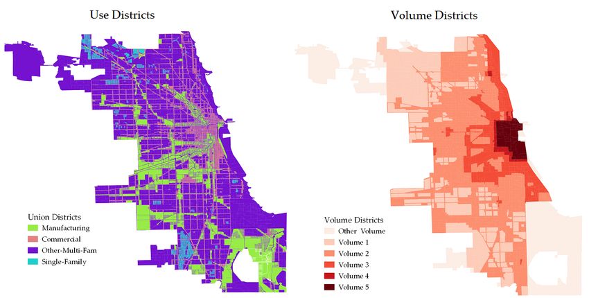
1        Introduction

Regulations on the use of land are prevalent in almost every city in the modern world, and their

effects on housing prices (e.g., Glaeser et al. (2005)), housing supply (e.g., Saiz (2010)) and other

local outcomes (e.g., Saks (2008); Shertzer et al. (2018)) have been widely studied in the literature.1

Most of this research follows a reduced-form analysis and does not consider the general equilibrium

and welfare effects of land use regulations (LUR). These effects are relevant since LUR potentially

affects wages, amenities and household location choices through their effects on the residential and

commercial real estate markets. On the other hand, recent research by Allen et al. (2015) study

the general equilibrium and welfare effects of zoning, but does not provide well-identified treatment

effects and does not consider the distributional effects of these policies .

        In this paper, I investigate the general equilibrium and distributional effects of zoning and floor-

to-area (FAR) restrictions within a city. In particular, I use a spatial quantitative model of a city,

together with well-identified reduced form estimates, to study the effects of these policies on real

estate prices, location choices and wages of low- and high-skilled workers, amenities, productivity,

land prices and welfare by skill type. Zoning and FAR restrictions are among the most popular

tools used by city governments to organize land use and economic activity. Specifically, zoning

specifies the permitted uses or activities inside a location, while FAR specifies the scale and volume

of these activities and is regarded as a good predictor for permitted building heights.

        Among other results, I find that an increase of 10 percentage points in the share of residential

zoning in a block group leads to a 1.7% increase in housing prices, a 5.4% and 5.8% decrease in the

wages of high-skilled and low-skilled workers, respectively, and a 5.1% decrease in local productivity.

On the other hand, an equivalent increase in the share of mixed-use designations leads to a decrease

of 5.4% in housing prices, a lower concentration of high-skilled residents, a 2.6% increase in wages

for both types of workers and a similar increase in local productivity. Relaxing FAR limits in a

location leads to lower housing prices and amenities, higher wages and productivity, and a higher

concentration of low-skill workers.
    1
   I am not aware of any large city without land use regulations. Even Houston, which is well-known for not having a
comprehensive Zoning Ordinance, uses other tools, such as restrictive covenants and deed restrictions (Siegan, 1970).

                                                         1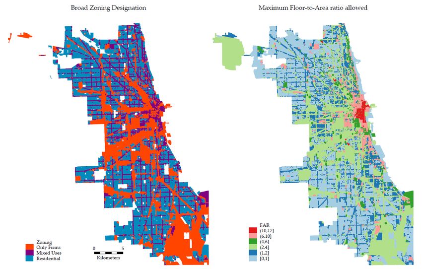
Since zoning and FAR restrictions affect sorting patterns and skill-specific wages, my findings

highlight the importance of including worker heterogeneity when studying the effects of LUR. In this

paper, I focus on the distinction between high- and low-skilled workers, which differ in at least three

dimensions. First, there are significant differences in real wages between both skill types within and

across urban areas (Baum-Snow and Pavan, 2013; Moretti, 2013). Second, low-income households

spend a higher share of their income on housing (Notowidigdo, 2019). Since low-skilled workers

are more likely to earn low wages relative to high-skilled workers (Mincer, 1974), higher housing

expenditure shares make them more susceptible to changes in housing prices. Third, high-income

workers have a higher opportunity cost of commuting time (Wheaton, 1977). These differences

affect the location choices of both types of workers and how they react to changes in LUR.

   To study these issues, I collect detailed geographic data for Cook County and the City of Chicago

for 2015-2016. These data include the universe of real estate transactions from Zillow (2017) and

the geographic distribution of zoning districts within Chicago. Using these data, I build residential

and commercial real estate price indices and different measures of LUR at the Census block group

level. I complement these data with data containing commuting flows and counts of people by

education category at the block level, and with Cook County’s Land Use Inventory CMAP (2016).

The real estate data show that residential and commercial prices are significantly different in more

than 90% of the block groups in the city. These price gaps indicate the existence of inefficiencies in

the real estate market and a potential welfare-improving role of changes in the zoning ordinance.

   Identification of causal effects of LUR is cumbersome given the endogeneity of zoning and FAR

regulations. For instance, low-density zoning is more likely to happen in neighborhoods with a

larger share of high-income population (Fischel, 2001), with more desirable amenities (Hilber and

Robert-Nicoud, 2013), or facing a lower demand for floor space (Wallace, 1988). I tackle these issues

using an instrumental variables approach, in which I instrument current regulations with the 1923

Chicago Zoning Ordinance. This ordinance was the first comprehensive zoning ordinance adopted

in Chicago. In particular, Shertzer et al. (2018) show that the 1923 Zoning Ordinance is a good

predictor of current zoning and current land uses. Following Shertzer et al. (2016a), who show that

1923 neighborhood demographic and geographic characteristic had an effect on the initial zoning

ordinance, I include in my analysis a large set of historical covariates.

                                                  2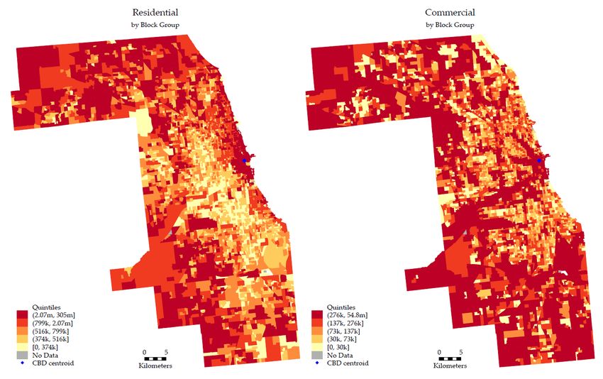
Afterward, I present a quantitative model of a city that builds on Ahlfeldt et al. (2015). Contrary

to their model, I introduce two types of workers: low- and high-skilled, who differ in their income

and housing expenditures. Moreover, in the spirit of Muth (1969) and Fujita and Ogawa (1982),

my model includes the microfoundations of a real estate market in which developers supply both

residential and commercial floor space subject to zoning and FAR restrictions. The inclusion of

developers and LUR into a spatial quantitative model constitutes an important contribution of my

paper. From the model, changes in welfare given by a change in LUR can be decomposed as the

sum of four effects: (i) changes in housing prices, (ii) changes in skill-specific amenities coming

from sorting, (iii) changes in wages and market access, and (iv) changes in the income coming from

the rents of land.

   Using this model, I follow the methodologies proposed by Ahlfeldt et al. (2015) and Tsivanidis

(2019) to recover block group measures of wages, amenities and productivity, given observed data

and values for the model’s parameters. Moreover, I lay out a solution for the equilibrium of the

real estate market. The proposed solution lets me recover land prices and the shadow price of FAR

regulations at the block group level. After recovering these unobservables, I study how zoning and

FAR restrictions affect them. Following the instrumental variables approach, I find that tighter

regulations in a block group lead to lower local wages. n particular, a 10 percentage points increase

in the share of residential zoning, relative to block groups with more commercial zoning, leads to a

decrease of 5.8% in the wage of low-skilled workers and of 5.4% in the wage of high-skilled workers.

The effect on wages of a one-unit decrease in FAR limits is a decrease of 19% for both types of

residents. These lower wages are compensated by increases in amenities of around 2.5% and 3%

for the respective policies. However, these policies also have a significantly negative effect on local

productivity of 5% and 18%, respectively.

   Finally, counterfactual exercises suggest an important role of changes in the zoning code for

improving welfare and decreasing inequality. In particular, I simulate the effects of four policies.

First, a policy that allows more residential zoning in block groups displaying an excess relative

supply of commercial real estate, and vice versa. Second, a policy that increases the FAR limit by

0.5 in those blocks where the constraint is the most stringent. Third, a policy that sets a minimum

FAR of 1.2 everywhere in Chicago. Fourth, a policy that sets a minimum of land zoned for mixed-

                                                  3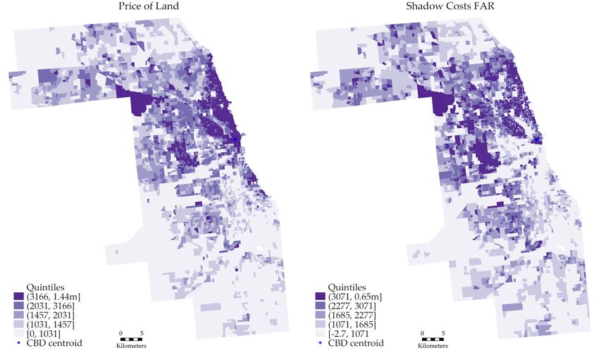
uses at 25% in each block group. All of these policies lead to similar welfare improvements for

low-skilled residents, and to a decrease in the welfare gap between skill types. These quantitative

exercises also suggest that the current zoning ordinance is a regressive policy that benefits high-

skilled residents more, but that it can be modified to reduce welfare inequality.

      This paper is related to the literature studying the effects of LUR.2 Theoretically, Helsley

and Strange (1995) and Rossi-Hansberg (2004) explore some welfare effects of LUR. Empirically,

most of the literature agrees that LUR leads to i) higher land and housing values, and to a more

inelastic supply of floor space (Mayer and Somerville, 2000; McMillen and McDonald, 2002; Glaeser

et al., 2005; Glaeser and Ward, 2009); and ii) to decreases in total welfare, with potentially large

distributional impacts (Cheshire and Sheppard, 2002; Turner et al., 2014; Hsieh and Moretti, 2015).

My paper also relates to research studying zoning in Chicago and the 1923 Zoning Ordinance

(McMillen and McDonald, 2002; Zhou et al., 2008; Shertzer et al., 2016a, 2018). In particular,

Shertzer et al. (2018) conclude that zoning in Chicago has been more important than geography or

transportation networks determining the distribution of economic activity. My paper contributes

to this literature by providing a general equilibrium evaluation of LUR. Specifically, by studying

the effects of zoning and FAR on a wide range of outcomes—i.e., housing and land prices, wages,

productivity, sorting and welfare—, I include in one single framework the effects of these policies.

      This paper also relates to the articles that explore heterogeneous effects of LUR. In particular,

Kahn et al. (2010) and Levine (1999) find that areas with more low-density zoning experience

more gentrification, affecting mostly minorities and low-income households. Muehlegger and Shoag

(2015) show that tighter LUR are associated with increases in commuting time, especially for

more educated and wealthier individuals. Ganong and Shoag (2017) find that stringent LUR in

productive cities has caused a decrease in the returns to living in these cities for low-skilled people,

but have remained constant for high-skilled. My paper contributes to this literature in three ways.

First, by analyzing the impact of LUR on the distribution of skills across locations within a city.

Second, by disentangling the effects that zoning and FAR restrictions have on wages and welfare

by skill type. Third, by contributing to the debate on whether zoning is a regressive measure,

benefiting high-skilled people more.
  2
      Fischel (2015) and Gyourko and Molloy (2015) provide superb summaries about the recent state of the literature.

                                                          4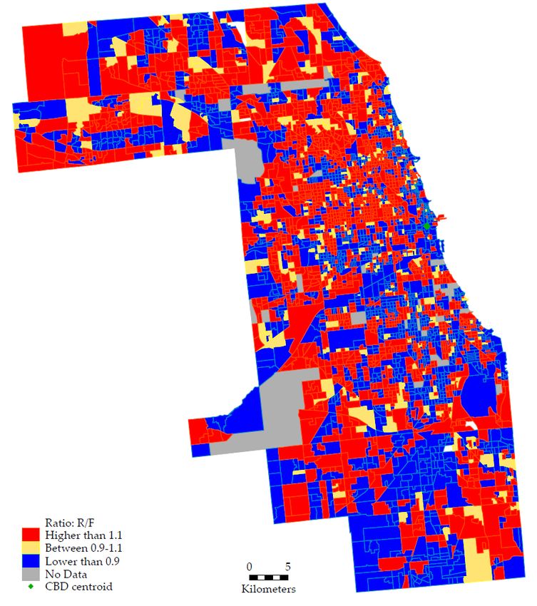
Furthermore, my paper is part of a recent literature using quantitative models in urban eco-

nomics such as Ahlfeldt et al. (2015); Allen et al. (2015); Tsivanidis (2019); Baum-Snow and Han

(2019), among others. There are three important departures of my model with respect to the stan-

dard models. First, similar to Tsivanidis (2019), my model includes worker heterogeneity, which

is important given the potential distributional impacts of LUR. Second, my model includes micro-

foundations for the supply of real estate supply into this quantitative setting. Third, I decompose

changes in welfare in changes in rent, wages, sorting and income from land rents, to study the

specific mechanisms through which LUR affects residents.

    The paper proceeds as follows. In Section 2, I describe my data sources. In Section 3, I briefly

discuss the 1923 Zoning Ordinance and study the relationship between LUR, real estate prices and

sorting by skill. Section 4 presents the quantitative model with heterogeneous workers and LUR.

Section 5 exploits the recursive structure of the model in order to solve the model, given some

data and values for different parameters. In Section 6, I explore the effect of zoning and FAR

restrictions on wages, amenities, productivity, and land prices. In this section, I also present the

policy counterfactuals that show how changes in LUR can lead to reductions in welfare inequality.

The final section concludes and highlights directions for future research.

2    Data and Descriptive Statistics

In order to investigate the effects of zoning and FAR restrictions on real estate prices, sorting and

wages across locations, I combine data from five sources. First, data on workplace and residence

area characteristics from the US Census Bureau. Second, data from Zillow Economic Research

containing the universe of real estate transactions. The LODES and Zillow data are available

for any city in the country. The main challenge constitutes finding a city with detailed data on

LUR. Fortunately, the Data Portal of the City of Chicago contains a database with all the zoning

districts within city boundaries, which I complement with a Land Use Inventory for the rest of

Cook County. Finally, I use historical zoning, demographic and geographic variables for Chicago

in the 1920s, collected and studied by Shertzer et al. (2016a), Shertzer et al. (2016b) and Shertzer

et al. (2018). In the rest of this section, I describe these data and present descriptive statistics.

                                                   5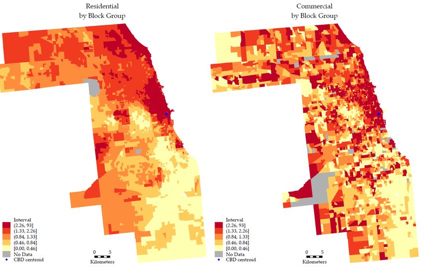
2.1      Real Estate Prices

I use data of real estate prices and stocks from Zillow Economic Research for Cook County in

2015 and 2016. The Zillow ZTRAX data are constructed from information in local deed transfers

and mortgages for mostly residential properties, but also include commercial properties in the more

recent years.(Zillow, 2017).3 Among other variables, these data include sales price, transaction date

and coordinates of the property. I merge this dataset with their assessment data, which include

property characteristics, geographic information, current and prior valuations.

       Using the ZTRAX transactions and assessment data, I build quality-adjusted residential and

commercial real estate price indices for each census block group in Cook County for 2015-2016

using a hedonic regression approach.4 Further details regarding the construction of these indices

can be found in Appendix A.1. The estimated residential price index covers around 97% of all

block groups in my sample, while the commercial price index has a coverage of 43%. To increase

coverage, I use an inverse distance weighted interpolation for those block groups with missing price

indices. For those blocks where missing values persists, I use the mean within the block group’s

census tract. These imputations raise the coverage of the residential and commercial price indices

to 99.9% and to 97.5%, respectively. Since these prices are identified up to scale, I normalize their

geometric mean to 1. Figure A1 presents the distribution of real estate prices across block groups

in Cook County, and Table A1 presents descriptive statistics.

       There is significant variation between residential and commercial real estate prices across loca-

tions. On average, residential real estate is more expensive than commercial, but 5.4% of the block

groups have commercial real estate more expensive than any block group’s housing. Moreover, the

data show that residential prices are higher than commercial prices in around 45% of the block

groups, commercial is more expensive than residential in 46%, and only in around 8% the ratio lies

between 0.9 and 1.1. The existence of these price gaps is interesting from a theoretical perspective

since canonical models of real estate supply suggest that developers provide both residential and
   3
     Data provided by Zillow through the Zillow Transaction and Assessment Dataset (ZTRAX). More information
on accessing the data can be found at http://www.zillow.com/ztrax. The results and opinions are those of the author
and do not reflect the position of Zillow Group.
   4
     A block group is the US Census classification lying between a tract and a block. There are 809 tracts in Chicago
containing on average 2.7 block groups, and there are 2,194 block groups containing on average 17 blocks.

                                                         6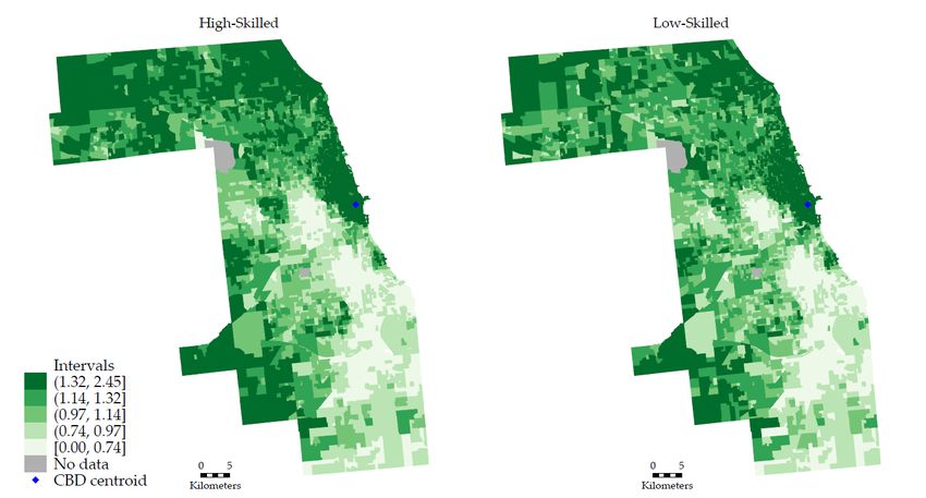
commercial floor space until their price equalize. Therefore, these gaps indicate the existence of

inefficiencies in the real estate market, and a potential role for changes in LUR to solve them.

Figure 1 shows the geographic distribution of such gaps.

        Figure 1: Real Estate Price Gap (Residential/Commercial)–Cook County, 2015-2016

This figure shows the ratio between residential and commercial real estate price indices for every block group in Cook
County for 2015-2016. These prices are estimated using a hedonic regression approach for both types of properties,
separately, and an inverse distance weighted interpolation for those locations without enough observations. Red block
groups are those where residential prices are at least 10% higher than commercial prices. Blue block groups are those
where commercial prices are at least 10% higher than residential prices. Yellow block groups are those where prices
are in the interval between the previous categories. Green dot represents Chicago’s CBD.

    Finally, I use the assessment data to measure the stock of residential and commercial floor space

in each block group as the sum of the built square footage of all properties within type. Figure A2

shows that the block groups with the largest stock of residential space are located downtown and

in the suburbs, while the stock of commercial real estate is concentrated downtown, along the main

avenues and in the suburbs.

                                                          7
2.2      Land Use Regulations

The data on land use and its regulations comes from two sources. First, from the Data Portal

of the City of Chicago, which contains a geographic database of all the zoning districts within

city boundaries. Second, from the 2015 Land Use Inventory for Cook County, which is built and

published by the Chicago Metropolitan Agency for Planning (CMAP).

       The zoning data contain the polygons and specific zone class categories in 2016. The detailed

specifications of each zone class are available in the Chicago Zoning and Land Use Ordinances (City

of Chicago, 2019). In total, there are 66 zone classes, 15 Planned Manufacturing Developments

(PMD) and more than a thousand Planned Developments (PD) within the city. Out of the total

land area in Chicago, around 52% is currently categorized as residential (R), while manufacturing

(M), commercial (C) and business (B) districts use approximately 11%, 3% and 7%, respectively.

Locations categorized as downtown districts (D) use about 1% of the area.5 PMD and PD cover

6% and 12%, respectively. Further details of this database can be found in Appendix A.2.

       I group all districts into three categories: those designated for residential purposes only, for

commercial only and for mixed-uses. I also categorize each Planned Development into a category

based on their characteristics.6 In the left panel of Figure 2, I present a map of Chicago using

this categorization. The land that can be used by firms only (red) is spread along and around the

main highways and waterways, while mixed-use areas (purple) are located mainly downtown and

along the main streets. Areas designated for residential purposes only (blue) are located mainly

in neighborhoods surrounded by mixed-use areas. In the right panel, I map the maximum FAR

allowed in each zoning district. High density (red and pink) is allowed mostly downtown and in

some parts of the coast; medium density (greens) is allowed along the coast of Lake Michigan and

in the areas where only commercial uses are allowed; low density (blues) is allowed particularly in

residential zoned areas.7

       Using these maps, I build block group measures of the share of land designated for residential,
   5
     Downtown districts can be Residential (DR), Core (DC), Service (DS) or Mixed-Use (DX) districts.
   6
     Planned Developments correspond to tall buildings and other large developments in which developers must work
with the City to ensure that the project integrates with surrounding neighborhoods (2nd City Zoning, nd). The City
of Chicago keeps pdf files for each Planned Development in https://gisapps.chicago.gov/gisimages/zoning˙pds.
   7
     In Figure A3, I present a map of the distribution of all nine broad zoning designations.

                                                        8
Figure 2: Land Use Regulations in Chicago
Notes: This figure shows two current land use regulations in the City of Chicago. The left map presents the
areas where only commercial (red), residential (blue) or mixed-uses (purple) are allowed. The right panel shows
the maximum FAR allowed in each zoning district, where reds denote high allowed density, greens denote medium
allowed density, and blues denote low allowed density.
mixed-uses or commercial purposes, and the average allowed FAR. I also build a measure of the
share of residential floor space allowed in each block group and denote it as λ.8 This measure is
used for solving the model as it captures the share of floor space in mixed-use districts that can be
used for housing.
The zoning data is only available for the City of Chicago, which contains around 35% of the
residents of its metropolitan area. Ignoring land uses outside the city might render an incomplete
picture of the effects of LUR on the distribution of economic activity in this labor market. For
this reason, I include data on the use of land in the rest of Cook County from the 2015 Land Use
8
For example, B3-3 zoning districts have an allowed FAR of 3, with apartments only permitted above the ground
floor. In this case, I assume that the first floor is used for commercial purposes, while the two remaining floors are
used for residential purposes. Hence, I set λ = 2/3. Moreover, λ = 1 for residential-only districts, and λ = 0 for
commercial-only districts.
9Inventory. This inventory contains the specific uses of land in all Northeastern Illinois and is built
to develop long-range population and employment forecasts that support Chicago Metropolitan
Agency’s planning strategies (CMAP, 2016). Using these data, I build measures of the share of
land area used for residential, mixed-uses or commercial purposes in each block group outside the
City.
In Table 1, I present descriptive statistics of the different measures of zoning across block groups
in Cook County. The average block group has 75% of its land zoned for residential purposes, 15%
for commercial purposes and 10% for mixed-uses. The average allowed FAR is 1.8. Furthermore,
out of the 10% zoned for mixed-uses, around 77% of it can be used for housing. Compared to the
average, the median block group is more residential and has lower FAR. In fact, 75% of the block
groups in the city have an average allowed FAR of less than two.
Table 1: Descriptive Statistics - Zoning Measures
Mean SD Min p25 p50 p75 max
Sh. Res. Only 0.75 0.24 0 0.66 0.83 0.93 1
Sh. Mixed-uses 0.10 0.15 0 0 0.02 0.14 1
Sh. Firm Only 0.15 0.21 0 0 0.06 0.21 1
Mean FAR 1.82 1.60 0.5 0.94 1.24 2.01 14.2
Sh. Res. Space Allowed 0.77 0.22 0 0.70 0.85 0.92 1
Notes: This table shows descriptive statistics for different measures of land use regulations across block groups for
Cook County in 2016.
For my empirical strategy, I also use the 1923 Zoning Ordinance together with a large set of
demographic and geographic characteristics from the early 1920’s. The 1923 zoning data was digi-
tized by Allison Shertzer, Tate Twinam and Randall Walsh, who provided me with the shapefiles
containing the four use-districts and the five volume-districts used in this ordinance. I provide fur-
ther details of this Ordinance in Section 3.1. Moreover, I use different demographic and geographic
data from the 1920 census, which is provided in the supplementary material from Shertzer et al.
(2016a). The authors collect these data at the enumeration district level from a variety of sources,
including Ancestry.com, National Archives and the 1922 Chicago Land Use Survey.
102.3 Distribution of Skills and Commuting
For data on population by workplace and residential areas, I use version 7.2 of the US Census Bureau
Longitudinal Employer-Household Dynamics (LEHD) Origin-Destination Employment Statistics
(LODES) for 2015 and 2016. The LODES data contain information about the location of jobs and
residences as provided by state unemployment insurance and federal worker earning records. These
data contain counts of the people living and working in each census block. This information can
be further split by earnings categories or educational attainment. The LODES data also contain
the number of commuters between every pair of blocks, which can only be separated by age and
earnings categories.
Out of the total working population of age 30 or older in Cook County in 2015-2016, 14% had
less than a high school degree, 23% had a high school degree only, 30% had a college or an associate
degree, and 33% had a bachelors or an advanced degree. I categorize as low-skilled those workers
within the first two categories. Table A2 presents the number of residents and workers by education
category in the mean and median block group. These statistics show that the distribution of workers
across block groups is more skewed than the distribution of residents. Figure A4 presents the share
of high-skilled people for every block group of residence and of work in the county. These maps
show a high concentration of high-skilled residents, especially in the downtown area and north of
it. Low-skilled residents are concentrated in the south and west portions of the county.
The LODES data also contain for each block the number of workers by skill type for three
earnings categories: less than $1250/month, $1250/month to $3333/month, and greater than
$3333/month. I define as high-wage those workers within the top category and calculate the share
of low- and high-wage workers by skill.9 Under this definition, approximately 37% of workers in
Cook county are in the high-skilled high-wage category, while 25% are in the low-skilled low-wage
category. Table A3 presents these shares.
9
According to the American Community Survey (ACS), out of the full-time year-round workers with positive
earnings, approximately 4.7% makes less than $1250 each month, 34.5% earns between $1251 and $3333, and 60.8%
makes more than $3333 a month.
113 Land Use Regulations, Prices and the Distribution of Skills
In this section, I explore the effects of zoning and FAR restrictions on the distribution of real
estate prices, wages and people by skill across block groups. Real estate prices and wages are
relevant outcomes since they affect households’ expenditures and income, and potentially welfare.
In addition, the distribution of people by skill across locations is relevant as local amenities and
productivity tend to respond positively to higher population density. Moreover, if each block group
is considered to be a small open economy, the spatial concentration of residents could be a rough
measure of local welfare. In order to identify the effects of current regulations, I use the 1923
Chicago Zoning Ordinance, together with an instrumental variables approach. I start by briefly
describing this ordinance, but the reader should refer to Shertzer et al. (2016a) and Shertzer et al.
(2018) for more detailed information.
3.1 The 1923 Chicago Zoning Ordinance
There are at least three threats to causal identification of the effects of land use regulations on the
spatial distribution of economic activity. First, low-density zoning is more likely in neighborhoods
with a larger share of high-income population. Since richer households are more likely to own
properties, if LUR leads to higher housing prices owners may want to strengthen the regulations
to increase the value of their homes. This phenomenon is known as the Homevoter Hypothesis
(Fischel, 2001; Parkhomenko, 2020). Second, locations with more desirable amenities (such as
parks, lakes or historical buildings) might have tighter LUR to prevent developments around these
areas (Hilber and Robert-Nicoud, 2013). Third, changes in zoning could be caused by changes in
the demand for certain locations (Wallace, 1988).
I tackle these issues by instrumenting current LUR using the 1923 Chicago zoning ordinance,
which was the first comprehensive zoning ordinance adopted in Chicago. Even though Chicago’s
city government had made previous attempts to control undesirable land uses, these approaches
were insufficient to meet public demand in a constantly growing city. Therefore, in 1921 the local
government created a Zoning Commission, which spent 18 months surveying existing land uses and
12organizing public hearings, until the final ordinance was adopted in 1923. The ordinance regulated
land by restricting allowed uses and building volumes: it included four use districts (single-family
residential, multi-family residential, commercial and manufacturing), and five volume districts, that
imposed restrictions on height and lot coverage.10 Figure 3 shows the distribution of use and volume
districts according to the 1923 zoning ordinance, which, according to. Shertzer et al. (2018), are a
good predictor of current LUR.
Figure 3: 1923 Chicago Zoning Ordinance
Notes: This figure the distribution of use and volumn districts given by the 1923 Chicago Zoning Ordinance. The left
map presents the four use districts: single-family residential, multi-family residential, commercial and manufacturing.
The right map presents the five volume districts.
Using the use and volume districts from the 1923 zoning ordinance, I build block group level
measures of the share of each district. I use these shares as instruments for 2016 LUR following
this specification:
LU R2016,i = πZoning1923,i + ψXi + i (1)
10
Use districts were hierarchical, which means that multi-family districts allowed single-family residences, commer-
cial districts allowed multi- and single-family residences, and manufacturing districts allowed any use.
13where LU R2016,i corresponds to one of the block group level measures of LUR in 2016 presented in
Table 1; Zoning1923,i is a vector that includes the 1923 shares of land designated as manufacturing
or commercial (single- and multi-family residential are the omitted categories), and as volume
districts 1, 2 or 3 (volume districts 4 and 5 are the omitted categories); Xi is a vector of control
variables at the block group level, which includes total land area, interactions between distance to
the CBD and the closest body of water,11 , a transit accessibility index,12 1927-wards fixed effects,
and a set of 1922 neighboorhood demographic and land use characteristics.13 This large set of
controls and fixed effects implies that I am comparing highly similar block groups inside 1927-
wards, thus, I am using rather local variation to identify the causal effects of zoning and FAR
restrictions. Demographic and economic characteristics are available for around 67% of the block
groups within Chicago. Therefore, identification of my estimates come from the impact of these
regulations in this portion of the city. Nonetheless, the quantitative exercises from Sections 5 and
6.4 use data for the entire county.
Finally, i corresponds to the error term. All of the regressions include spatial heteroscedasticity
and autocorrelation consistent (SHAC) standard errors (Conley, 1999). Specifically, I use the
routine developed by Hsiang (2010) with a linear Bartlett window. I calibrate the distance cutoff
of the spatial kernel to 1.5 km based on results derived from bootstrapping the spatial correlation
between residual real estate prices. I present these results in Figure A5 and show that the residual
covariance between real estate prices is almost zero among block groups located 1.25 and 1.75km
away, for residential and commercial real estate prices, respectively.
I present the estimation results from equation (1) in Table 2. Columns (1)-(2) use as dependent
variables the share of land where only residential or mixed-uses are allowed. Results from these
columns are similar to those from Table A.4 in Shertzer et al. (2018): block groups with a higher
11
Including Lake Michigan, Chicago River (south and north branches), Des Plaines River, Little Calumet River,
and a small number of large lakes within city boundaries.
12
The raster map used to compute this index was provided by Tate Twinam, who obtained it from
www.walkscore.com.
13
I use the same set of control variables from Shertzer et al. (2016a) and Shertzer et al. (2018). These controls
are: percent of northern- or southern-born black population; percentage of first- or second immigration immigrants;
population density; maids per household; indicator for presence and distance to a major street, coast, main or ancillary
railroads, and Union Stockyards; number of warehouses; indicator and density of commercial uses, manufacturing
uses, 4,...,10,11-25 story buildings; number of manufacturing uses within 500ft and between 500ft and 1000ft; indicator
for alderman living in district; 1913 land values.
14share of land designated for manufacturing and/or commercial purposes in the 1923 ordinance have
a larger share of land zoned for residential-only uses in 2016, relative to similar and nearby block
groups with a lower share of these designations. Moreover, these blocks have a higher share of land
zoned for mixed-uses. Column (3) shows that block groups with a higher share of land designated
for manufacturing and/or commercial purposes in the 1923 ordinance have high allowed FAR today.
Regarding volume, a larger share of low volume districts in 1923 is associated with lower FAR limits
in 2016, relative to block groups with a larger share of high volume districts in 1923.
Table 2: First Stage Regressions: 2016 Zoning as a Function of 1923 Zoning
(1) (2) (3)
Sh. Only Sh. Mixed Mean
1923 / 2016 Residential Uses FAR
Share Commercial -0.37*** 0.41*** 0.51***
(0.00) (0.00) (0.00)
Share Manufacture -0.44*** 0.03*** 1.09***
(0.00) (0.00) (0.00)
Share Volume 1 -0.13*** 0.11*** -1.83***
(0.00) (0.00) (0.00)
Share Volume 2 -0.15*** 0.12*** -1.57***
(0.00) (0.00) (0.00)
Share Volume 3 -0.13*** 0.07*** -1.01***
(0.00) (0.00) (0.00)
R-squared 0.96 0.80 0.93
Notes: This table shows the results of regressions of 2016 measures of land use regulations as function of the share
of allowed uses and volumes given by the 1923 Chicago Zoning Ordinance. These measures are constructed at the
block group level. Omitted 1923 zoning types are residential uses and volume districts 4 and 5. (1)-(2) correspond to
the share of land in districts where only residences or mixed-uses are allowed, respectively. The share of land where
only firms are allowed is the omitted category. (3) corresponds to the mean FAR. Number of block groups is 1,427.
Spatial Heteroscedasticity and Autocorrelation Consistent (SHAC) standard errors in parentheses (Conley, 1999);
*** pwhere ln(rT i ) corresponds to the quality-adjusted price index for type T properties (residential
or commercial) in block group i; LU R2016,i corresponds to one of the measures for current LUR;
Xi denotes the set of control variables described in equation (1); ε1i is the error term. The OLS
estimates from equation (2)–which are presented in Table A4–show a non-significant relationship
between LUR and real estate prices. As discussed previously, these estimates could be biased
since homeowners in locations with high housing prices may lobby for more stringent regulation to
maintain high prices.
Therefore, I estimate equation (2) using two-stage least squares (2SLS), where the first stages
are given by equation (1). Identification under this strategy requires that historical LUR only affect
real estate prices through their impact on current LUR, once controlling for the set of historical and
geographic characteristics. Ward fixed effects and controls imply that the estimates from my 2SLS
regressions are identified using within-wards variation, comparing block groups that were similar
in terms of 1920 demographic and current geographic characteristics, but differ in their current
regulations.
Table 3 presents the results of these regressions. Estimates from Panel A suggest that block
groups with a larger share of area designated for residential uses have higher residential prices and
built area. In particular, an increase of 10 percentage points (pp) in the share of residential-only
area (e.g., going from the median to the 75th percentile block group) leads to a 1.7% increase in the
average price of housing, relative to block groups with more commercial-only designations. This
increase also leads to a 3.5% increase in the price of commercial real estate. A similar increase in
the share of mixed-use zoning leads to reductions of 5.4% and 4.6% in residential and commercial
prices, respectively. In Panel B, I show that a one-unit increase in the mean allowed FAR leads to
a decrease of 2% in housing prices, but a 5% increase in the price for commercial real estate. The
weak effect of more relaxed FAR on housing prices can be driven by two effects: an increase in the
stock of floor space (as suggested by Column 2), together with a potential increase in population
density, which could lead to more amenities. The positive effect for commercial prices could be
driven by increases in productivity brought by a higher density of workers and businesses.
16Table 3: Effects of LUR on the Real Estate Market
(1) (2) (3) (4)
Ln Price Ln Stock Ln Price Ln Stock
Type Residential Commercial
Panel A
Sh. Res. Only 0.17*** 1.11*** 0.33*** -2.05***
(0.00) (0.00) (0.00) (0.00)
Sh. Mixed-uses -0.56*** 0.66*** -0.48*** 12.91***
(0.00) (0.00) (0.00) (0.00)
F-Test 13.09 11.86 15.31 11.86
Panel B
Mean FAR -0.02*** 0.12*** 0.05*** 0.97***
(0.00) (0.00) (0.00) (0.00)
F-Test 20.06 18.61 20.59 18.61
Observations 1,424 1,421 1,376 1,421
Notes: This table shows the results of 2SLS regressions of the effects of different LUR measures on prices and stock
in the real estate market. The estimations use the 1923 zoning ordinance as instrument and include controls for
block group’s land area, distance to the CBD and to major waterways, transit access, and historical covariates. Price
measures are quality adjusted (hedonic) and are defined in Section 2.1. Spatial Heteroscedasticity and Autocorrelation
Consistent (SHAC) standard errors in parentheses (Conley, 1999); *** pin Columns (1)-(3) and Columns (4)-(6) from Table 4.14
The results from Panel A suggest that, a 10pp increase in the share of land zoned for residential-
only uses leads to a small (but significant) increase of 0.2% in the share of high-skilled residents,
relative to block groups with more land zone as commercial-only. Estimates in columns (2) and
(3) suggest that more residential zoning also leads to more spatial concentration of both types of
residents relative to every other block group in the city. On the other hand, a 10pp increase in
the share of land zoned for mixed-uses in a block group, leads to a decrease of 1% in the share
of high-skilled residents. This change in skill composition comes from an increase of 8.3% in the
spatial concentration of low-skilled residents inside the block group, relative to an increase of 6.4%
in the spatial concentration of high-skilled residents. Columns (5) and (6) show that increases in
mixed-use zoning lead to increases in the spatial concentration of both types of workers.
Regarding FAR, Panel B shows that a one-unit increase in the allowed FAR leads to spatial
decentralization of residents and to a spatial concentration of workers, especially low-skilled. In
particular, a one-unit increase in the allowed FAR leads to 78% and 92% increases in the relative
spatial concentration of high-skilled and low-skilled workers, respectively. This result suggests that
higher FAR is associated with more mixed-use or commercial zoning, relative to residential.
Finally, I investigate the effect of current LUR on the distribution of wages for both types of
workers estimating the following regressions:
ShLowW agee,i = β3 LU R2016,i + ψ3 Xi + ε3,i , (4)
where ShLowW agee,i denotes the share of low wage workers from skill type e in block group i.
Columns (1) and (2) from Table 5 presents the results of these regressions for low- and high-skilled
workers, respectively.
Results from Panel A suggest that block groups with a higher share of area zoned for residential
or mixed-uses have a higher share of low-wage workers, both low- and high-skilled. In particular, a
14
Not controlling for the endogeneity of LUR could also lead to biased coefficients in these regressions, since
locations with a larger share of high-skilled and high-income residents may have more influential groups lobbying for
more stringent regulation. Columns (5)-(10) from Table A4 confirms the existence of these biases.
18Table 4: Effects of LUR on the Distribution of Skills
(1) (2) (3) (4) (5) (6)
Sh. High Sh. Low Sh. High Sh. High Sh. Low Sh. High
Skilled (w) Skilled (a) Skilled (a) Skilled (w) Skilled (a) Skilled (a)
Block Type Residence Work
Panel A
Sh. Res Only 0.02*** 0.98*** 1.06*** 0.10*** -2.91*** -2.36***
(0.00) (0.00) (0.00) (0.00) (0.00) (0.00)
Sh. Mixed-uses -0.10*** 0.80*** 0.62*** -0.03*** 0.95*** 1.16***
(0.00) (0.00) (0.00) (0.00) (0.00) (0.00)
F-Test 11.77 12.89 12.89 12.21 12.89 12.89
Panel B
Mean FAR 0.00*** -0.14*** -0.14*** -0.04*** 0.92*** 0.78***
(0.00) (0.00) (0.00) (0.00) (0.00) (0.00)
F-Test 19.04 20.42 20.42 20.82 20.42 20.42
Observations 1,423 1,427 1,427 1,389 1,427 1,427
Notes: This table shows the results of 2SLS regressions of the effects of different LUR measures on the spatial
distribution of high- and low-skilled workers within and across block groups of residence (Columns 1-3) and work
(4-6). The estimations use the 1923 zoning ordinance as instrument and include controls for block group’s land area,
distance to the CBD and to major waterways, transit access, and historical covariates. Dependent variables are in
logs; (w) denotes the share within block group (e.g., high-skilled as proportion to the block group’s population);
(a) denotes the share across blocks (e.g., high-skilled in a block group relative to the total high-skilled in the city).
Spatial Heteroscedasticity and Autocorrelation Consistent (SHAC) standard errors in parentheses (Conley, 1999);
*** pTable 5: Effects of LUR on Wages
(1) (2)
Sh. Low Wage
Skill Cat. Low High
Panel A
Sh. Res. Only 0.38*** 0.54***
(0.00) (0.00)
Sh. Mixed-uses 0.42*** 0.32***
(0.00) (0.00)
F-Test 12.11 12.21
Panel B
Mean FAR -0.10*** -0.18***
(0.00) (0.00)
F-Test 20.14 20.82
Observations 1,389 1,389
Notes: This table shows the results of 2SLS regressions of the effects of different LUR measures on the log share of
low wage workers by skill type. The estimations use the 1923 zoning ordinance as instrument and include controls
for block group’s land area, distance to the CBD and to major waterways, transit access, and historical covariates.
Spatial Heteroscedasticity and Autocorrelation Consistent standard errors in parentheses (Conley, 1999); ** pmicrofoundations for the real estate market by modelling real estate developers who face LUR and
choose the supply of real estate subject to these regulations.
Consider a closed city consisting of a set {1, 2, ..., L} of block groups, each with a total land
area of Li . The closed-city assumption implies that the city-wide population of each skill group is
exogenous, but the expected utility is endogenously determined. Block groups differ in terms of
final good productivity, residential amenities and their access to the rest of the city. Throughout
this section, residence locations are indexed with i or m, and work locations with j or n.
4.1 Individuals
There are two types of people: high-(s) and low-skilled (u), with a fixed total population of Ns and
Nu , respectively. Both types receive income from their labor and rents from land, which are paid
to every individual in the city. Individuals are indexed by o and are endowed with one-unit of labor
that is supplied inelastically. Every worker o of type e ∈ {s, u} living in location i and working in
location j faces a commuting cost dij > 1 and solves:
βe 1−βe
cio hRio
max uijeo = Bei vieo (5)
cio ,hRio βe 1 − βe
wej
s.t. cio + rRi hRio ≤ yeij = jeo + ϕe ,
dij
where Bei denotes skill-specific residential amenities and reflect the average preference of living in i
by type e residents; hRio and cio represent the amount of housing and final good demanded by worker
o living in block group i. Commuting costs act as a dispersion force, reducing the productivity
and wages at work. I assume these costs take an iceberg form dij = eκτij ≥ 1, where τij ∈ [0, ∞)
represents travel time between two locations and κ represents the incidence of these commuting
costs. In addition, individuals receive productivity shocks over workplace locations (jeo ) and
preference shocks over residential locations (vieo ), which differ by skill-type. Furthermore, I assume
βs ≥ βu following recent literature showing that low-skilled spend a higher share of their income
on housing relative to high-skilled people (Notowidigdo, 2019; Ganong and Shoag, 2017).
21In the budget constraint, the price of consumption goods is the same across locations and is
normalized to one; and rRi is the price of housing in location i. In this model, all land is owned
by people. Therefore, total income comes from their commuting-discounted wage wej /dij , plus a
transfer (ϕe ), which represents the payments received by households from the rents of land. These
transfers do not vary across space and are the same for all residents within skill type. I assume
that these payments are larger for high-skilled residents (ϕs > ϕu ).15 The sum of these payments
across all workers must equal total land rents, R = L
P
i (pi Li ), where pi denotes the price of the
land in location i.
From the solution of the maximization problem in equation (6), I obtain an expression for the
indirect utility of a worker o:
wej 1−βe
uijeo = Bei jeo + ϕe rRi vieo . (6)
dij
Given this indirect utility, individuals first choose where to live and then where to work. For the
second stage, assume that type e residents from location i draw a vector of iid match-productivities
over workplace locations from a Fréchet distribution with cdf F (je ) = exp{−Te −θ
je }. The scale
e
parameter Te determines the average productivity of type e workers and θe > 1 the dispersion of
worker productivity within type, with a higher θe implying a lower degree of unobserved hetero-
geneity. Residents choose the work location that offers the highest commuting-discounted wage:
maxj {wej jeo /dij }. Properties of the Fréchet distribution imply that the probability of a type-e
resident of working in location j conditional on living in i is:
θe −κθe τij θe −κθe τij
Neij wej e wej e
πj|ie = = PL θ
= . (7)
NRei e
n=1 wen e
−κθ τ
e in RM Aei
This probability depends positively on the wage offered in that location net of commuting costs,
relative to all other locations. Differences in the dispersion parameters θs and θu determine differ-
ences in the incidence of commuting costs across skill groups. In addition, RM Aei denotes block
group i’s residential market access of type e workers and is defined as RM Aei = L θe −κθe τin .
P
n=1 wen e
This measure summarizes the access to employment opportunities of type e residents of block i.
15
According to the 2015 5-year ACS, around 48% of low-skilled households in Cook County lived in their own
home, compared to 61.4% for high-skilled households. This latter group also received a larger amount of rent income.
22Since there is a continuum of agents, by the law of large numbers this probability also corresponds
to the number of type e individuals living in i and working in j (Neij ) relative to the total type-e
residents from location i (NRei ).
Before productivity shocks are revealed, the expected income of type e residents living in i is:
1/θe
ȳei = T̃e RM Aei + ϕe , (8)
1/θe 1
where T̃e = Te γθe , and γθe is the gamma constant evaluated at 1 − θe . This expression suggests
that workers receive higher income in locations with better access to jobs, as measured by RMA.
In a first stage, individuals choose their residential location by drawing a vector of iid preference
−ηe
shocks over locations from a Fréchet distribution with cdf F (vie ) = exp{−vie }. Properties of the
Fréchet distribution imply that the expected utility of a type e resident of the city is:
" L
#1/ηe
ηe
−η (1−βe ) ηe
X
ūe = γηe rRme Bem T̃e RM A1/θe
em + ϕe , (9)
m=1
1
where γηe is the gamma constant evaluated at 1 − ηe . This expression shows that the expected
utility of a type e city dweller depends on the average price of housing, the average expected income
and the average skill-specific amenities received across all locations. Similarly, the probability that
a type e resident chooses to live in location i is
−η (1−β )
ηe 1/θ
NRei rRi e e
Bei (T̃e RM Aei e + ϕe )ηe
πRei = =P −ηe (1−βe ) ηe 1/θ
, (10)
Ne L
Bem (T̃e RM Aem e + ϕe )ηe
m=1 rRm
which also corresponds to the number of type e residents in location i (NRei ) relative to the city
total (Ne ). This expression suggests that locations with relatively more amenities, lower rents and
higher residential market access are more desirable and attract more residents.
Commuting market clearing requires that the measure of type e workers employed in each
location j equals the measure of type e residents commuting to j:
L L θe −κθe τij
X X wej e θe
NF ej = πj|ie NRei = PL θe −κθe τin
NRei = wej F M Aej , (11)
i=1 i=1 n=1 wen e
23where F M Aej denotes firm market access, which measures the access to type e workers by firms in
location j, and is greater when a location is close from highly populated residential locations. In
particular, F M Aej and RM Aei can be defined as:
L L
X e−κθe τij NRei X e−κθe τij NF ej
F M Aej = , RM Aei = . (12)
RM Aei F M Aej
i=1 j=1
Finally, total demand for residential floor space by type e residents is given by:
(1 − βe ) 1/θ
HRei ≡ E[hRei ]NRei = T̃e RM Aei e + ϕe NRei . (13)
rRi
As expected, demand for housing depends positively on the mass of residents of each type and their
expected income, and negatively on the price of residential floor space in that location.
Amenities
Amenities are an important factor determining residential location choices. For instance, Bayer
et al. (2007) show that households are willing to pay more to live in locations with a high density of
high-skilled workers. On the other hand, residents of locations with more natural amenities, may
prefer lower population densities. I assume that amenities in a location depend on two components:
residential fundamentals and residential externalities. The first one, denoted by bei , captures fea-
tures of physical geography that affects the willingness to live in location i by type-e residents. The
latter, represents how population density of high-skilled residents affect amenities.16 In particular,
amenities in location i are given by:
σe
NRsi
Bei = bei , (14)
Li
where Li denotes land area, and σe controls the relative importance of externalities in overall
residential amenities by type e individuals.
16
I assume that both components are skill-specific as recent evidence suggest that different types of workers have
heterogeneous valuation for different types of amenities (Albouy, 2016; Couture and Handbury, 2017).
244.2 Firms
Firms produce a single final good under perfect competition and constant returns to scale. The
final good is costlessly traded, and is produced using floor space and both types of labor according
to the production function:
Yj = Aj ÑFαj HF1−α
j ,
h i1
where ÑF j = αu NFρ ju + αs NFρ js corresponds to the effective units of labor force used by firms
ρ
in location j and is a CES aggregator over low- and high-skilled workers with an elasticity of
1
substitution of 1−ρ ; HF j corresponds to commercial floor space; Aj is the block group-specific
productivity, which is exogenous to firms, but endogenous in the model; α = αu + αs denotes the
total labor share, and αe the share of type e labor.
Firms in location j choose the quantity of inputs that maximize their profits, taking wages
(wju , wjs ) and commercial real estate prices (rF j ) as given. From the first order conditions, the
following expressions show how firms substitute between both types of labor and the demand of
total effective labor:
wju NF1−ρ
ju wjs NF1−ρ
js
= , (15)
αu αs
1 −ρ 1 −ρ
1−ρ
1 ρ(1−α)
1−ρ 1−ρ 1−ρ 1−ρ
ÑF j = (αAj ) 1−α αu wju + αs wjs HF j . (16)
Note that labor demand in location j increases when local productivity or the amount of floor space
increase, or when wages decrease. Finally, using the zero profit condition, I derive the equilibrium
price of commercial floor space in location j, which shows that firms are able to pay higher rents
in locations with higher productivity and/or lower wages:
1
1 −ρ 1 −ρ
α(1−ρ)
α ρ(1−α)
1−α 1−ρ 1−ρ 1−ρ 1−ρ
rF j = α 1−α (1 − α)Aj αu wju + αs wjs . (17)
Productivity
25I assume that local productivity depends on two components: (i) production fundamentals
from location j (aj ), and (ii) production externalities of both types of workers, as captured by their
density in that location.17 Specifically,
δu δs
NF uj NF sj
Aj = aj , (18)
Lj Lj
F /L and N F /L correspond to employment density of low- and high-skilled workers in
where Nuj j sj j
location j, respectively; and δu and δs control the relative importance of skill-specific externalities
on determining productivity.
4.3 Real Estate Market with LUR
Based on the canonical models of housing in Muth (1969) and Fujita (1989), I present a simple
model of the real estate market with, with developers and LUR. In order to produce floor space,
developers use capital and land with a production technology that exhibits constant returns to
scale. Furthermore, assume that the owners of capital do not live in the city and that the price of
capital is determined in a national market and normalized to one.
Total demand for residential and commercial floor space in every block group is given by the
solutions of the residents’ and firms’ optimization problems. Given these assumptions, in a world
with no LUR, developers would build floor space for the group of agents (residents or firms) with
the highest willingness to pay, until the price of commercial and residential floor space equalize.18
Rent equalization leads to an optimal distribution of land between residential and commercial uses.
However, when city authorities regulate the use of land, the price of both types of floor space could
differ in equilibrium, and these depend on local demand conditions and LUR.
To incorporate these forces into the model, consider a Zoning Ordinance given by the matrix
Z ∈ {ωR , ωF , ωM , λ, h̄R , h̄F , h̄M }, where ωT is a vector containing the shares of land that can be used
for type T space (residential, mixed-use, commercial) in every block group, with ωRi +ωM i +ωF i = 1;
17
The standard interpretation of these externalities is that density facilitates knowledge spillovers, input sharing
or labor market pooling. See Rosenthal and Strange (2004) for a detailed review on agglomeration economies.
18
This is the implicit assumption in recent quantitative models, such as Ahlfeldt et al. (2015) and Tsivanidis (2019).
These models include a residual that rationalizes price differences.
26You can also read


