Commute Time and Labor Supply - Global Research Unit Working Paper #2018-015
←
→
Page content transcription
If your browser does not render page correctly, please read the page content below
Global Research Unit
Working Paper #2018-015

Commute Time and Labor Supply

Sumit Agarwal, National University of Singapore
Elvira Sojli, Univerity of New South Wales
Wing Wah Tham, Univerity of New South Wales

© 2018 by Agarwal, Sojli and Tham. All rights reserved. Short sections of text, not to
exceed two paragraphs, may be quoted without explicit permission provided that full
credit, including © notice, is given to the source.
Commute Time and Labor Supply

                        Sumit Agarwal1, Elvira Sojli2 and Wing Wah Tham2

                                                Abstract
Commuting imposes financial, time and emotional cost on the labor force, which increases the
cost of supplying labor. Theory suggests a negative or no relation between travel and working
time for two reasons: travel time is a cost to supplying labor and commuting frustrates the
traveler decreasing productivity. We use a unique dataset that records all commuting trips by
public transport (bus and train) over three months in 2013 to study if commuting time affects
labor supply decisions in Singapore. We propose a new measure of commuting and working
time based on administrative data, which sidesteps issues related to survey data. We document
a causal positive relation between commute time and the labor supply decision within
individuals. Specifically, we show that a one standard deviation increase in commute time
increases working time by 2.6%, controlling for individual, location, and time fixed effects.
There are two sources of variation in the elasticity of work time to travel time: across
individual and within individual (time variation). While part of the cross-sectional variation
may be captured by survey data, the time-variation is completely unexplored. First, we find that
the cross-sectional variation depends on whether one engages in a service or manufacturing
type of job. This cross-sectional variation might be missed out in survey-based responses due
to a different selection process, based say on the proportion of industries in the S&P500.
Second, we find that there is very large within individual variation in the elasticity, not based
on calendar effects, like day of the week or month.
We investigate several potential explanations for this result. We find that in professions where
interaction with co-workers and with customers is necessary, i.e. service jobs, disruptions in
travelling to work cause a backlog and increase the working hours beyond the original travel
delay. These (travel delayed) individuals are not compensated for the time that they put in, in
addition to the usual number of working hours. This means that there is a cost shift from
employer to employee. Given the recent trend of moving from manufacturing to service-based
economies, it is most likely the positive elasticity will increase and become a larger economic
burden.

JEL classification: D1, J22, J24, M54
Keywords: Commute time, labor supply, elasticity, task juggling, trains, buses, big data.

__________________________________________________________________
*We appreciate comments and suggestions from Souphala Chomsisengphet, Denis Fok, Dan Hamermesh, Decio
Coviello, Jessica Pan, Ivan Png, Nagpurnanand Prabhala, Wenlan Qian, Tarun Ramadorai, David Reeb, Amit
Seru, Bernard Yeung, and conference and seminar participants at the AEA 2018, National University of
Singapore, and Tinbergen Institute. All errors are our own.

1. Departments of Finance, National University of Singapore, BIZ1-07-69, Mochtar Raidy Building, 15 Kent
Ridge Drive, Singapore, 119245, Singapore (email: ushakri@yahoo.com).
2. School of Banking and Finance, UNSW Business School, University of New South Wales.
“Time spent travelling during normal work hours is considered compensable work time.
Time spent in home-to-work travel by an employee in an employer-provided vehicle, or in
activities performed by an employee that are incidental to the use of the vehicle for
commuting, generally is no “hours worked” and, therefore, does not have to be paid.”
– United States Department of Labor

1.   Introduction

Time is likely to be the most expensive and important commodity for an individual, and it has
become more expensive as wage rates and GDP/capita have increased. Thus, the opportunity
cost of each unit of time not spent working has increased, while the hours in a day remain
constant. An important question in economics is how do we value time? A rich literature has
developed looking at one aspect of the value of time - time spent travelling. This large
literature (see Zamparini and Reggiani (2007) and Hamermesh (2016)) finds that the value of
time as a percentage of hourly earnings has increased by more than 50% in the last 50 years. In
this study, we use travel data to answer an important economic question: what is the elasticity
of working time to travel time? Answering this question might help in answering related
questions of how much leisure or home production time is valued in comparison to working
time.

While most governments and Ministries of Labor do not consider travel time part of working
time, economists have assumed that economic agents do. Cogan (1981), and subsequently
textbooks in labor economics (e.g. Ehrenberg and Smith, 2003), assume that the number of
workhours is optimally chosen given the commuting distance, which implies that labor supply
is optimally chosen per day. Theory suggests that individuals account for commuting time as
part of their work time (e.g. Becker, 1965; Cogan, 1981) and large commuting times may even
impede labor force participation (Cogan, 1981). In other words, as the commute time increases
individuals will spend less time at work.

Empirically, it is hard to document the relation between commute time and labor supply, due to
lack of reliable information on travel time.1 So far, the literature on the allocation of time is
based on survey data.2 While the use of survey data is very valuable in conducting economic

1
  Cogan (1981) examines empirically the effect of labor costs on labor supply and concludes that increases in daily
fixed costs of work (e.g. commute costs) will reduce labor supply, at least for the sample of 898 married women,
who work some time in 1966, that he analyses.
2
  See Juster and Stafford (1991), Aguiar and Hurst (2007) and Aguiar, Hurst, and Karabarbounis (2012) for
surveys of the literature. More recently, Bick, Brüggemann, and Fuchs- Schündeln (2016, 2017) construct survey
based working hour data that are comparable across countries. Analysis and discussion of this data can be found in
Bick and Fuchs- Schündeln (2017, 2018).

                                                       1
research, with the availability of administrative datasets and computing power, one can study
these questions with better precision and document within person dynamic effects of the
relation between commuting time and labor supply decisions.3 This paper uses exactly such
administrative data to investigate the sign and magnitude of the relation between commute and
working time. However, we also supplement our analysis with travel-related survey data.

In recent years, individuals are spending more and more of their time commuting (to and from
work). For example, in the UK the number of people spending more than two hours travelling
to and from work every day has jumped by 72% to more than 3 million, from 2004 to 2014,
and the average commute time has increased from 45 to 54 minutes in this time period. In the
US, the mean one-way travel time to work has increased by 18% to 26 minutes in 2013, while
it was less than 22 minutes in 1980 (US Census Bureau, 2011 and 2014). The increase in
commute time implies that there has been a substantial increase in explicit (time and petrol)
labor supply costs. While, there have been some changes by employers to have flexible
working hours and ability to work from home, these have not reduced the overall cost of
commuting.

In addition to the pure monetary costs of commuting (petrol and public transport prices) and
opportunity cost of time spent commuting, there is psychological evidence, which shows that
commuting time is causing stress, tiredness, “road rage”, and general unhappiness (Novaco and
Gozales, 2009; Gallup-Healthways Well-Being Index 2009-2010; Kahneman et al., 2004). In
particular, Kahneman, Krueger, Schkade, Schwarz and Stone (2004) document that commuting
is the least satisfying activity of all type of daily activities, which generates feelings of
impatience and fatigue. In their study, increased commuting time is associated with increased
blood pressure and musculoskeletal problems, lower frustration tolerance, and higher levels of
anxiety and hostility. Hence, increased commuting time not only increases the time and
monetory cost of labor supply but also affects one’s productivity at work, which has
implications for the productivity and profitability of firms. Overall, studying the relation
between commute time and labor supply is a first order question both from an urban and labor
productivity point of view.

3
  Both approaches have their strength and weaknesses. For instance, using survey data may have non-
representative samples, selection bias, attrition rates, changing survey subjects, non-comparable samples across
countries, and under/over estimation of work time (propensity to supply conventional numbers of work hours).
Administrative data also has significant limitations. For instance, we do not get a comprehensive view of the
individual’s decision to commute, and we cannot observe the exact location of the home and work location.
Therefore, we see the use of these two datasets as complementary and not substitutes. Indeed, in this paper we use
both survey and administrative data for our analysis.

                                                       2
In this paper, we use two different datasets from Singapore. The first is a travel-related panel
survey dataset over three waves from 2004 to 2012. This is very detailed data on the modes of
transportation, travel time, and individual characteristics similar to the US Time Use Survey.
This data allows us to measure the travel time to work and non-work related activities based on
types of jobs and individual characteristics. The second is a unique dataset of all 6 million
electronic travel cards (EZ-Link card) in Singapore, from August to October 2013, which we
use to study the relation between commute time and labor supply.4 The EZ-Link cards provide
us with a wealth of information to study this relation. For instance, the cards are distinct for
adults, children, and pensioners, which allows us to accurately identify working adults.
Additionally, the cards document the time and location of embarkation and disembarkation of
the cardholder and the mode of transportation used (bus and/or train).5 This allows us to
measure the exact commute time of the passenger on public transport, as well as to determine
the time at work. The exogenous variation in the duration of each ride, i.e. delay due to traffic
congestion or MRT breakdowns, hence exogenous shock to travel time within individual, while
traveling to work enables the causal study of the effect of travel time on working time. The bus
(public transport) stop can be precisely linked to the postal code in an area, which is linked to
information on the nature of the destination (residential area, industrial area, central business
district), to the survey data on individual characteristics at the block level, and to weather
stations for localized weather information at the block level.
The time at work is measured imprecisely, because we estimate the time spent at work by the
use of the EZ-Link card, which can potentially be problematic in the cross-section. However,
since we can follow the same individual over time, the imprecision is less of a concern, unless
the imprecision is correlated with commute time within an individual.6 On the other hand, our
measure of commute time and working time reduces measurement issues related to non-
representative sample, recall/reporting bias, changing survey subjects, attrition rates, as well as
accounting for within individual effects.
4
The population of Singapore is 5.5 million. There are more EZ-link cards than the population because tourists
can also purchase these cards.
5
While we do not have precise information on race, nationality, cultural background, family size, residence status,
and occupation of the commuter, we can infer these from the location of residence. We discuss this further in the
data and results section.
6
In other words, does the imprecision of working time increase when the commute time increases? Specifically,
we attribute all the time spent once an individual leaves the train or bus in the morning until he/she gets back on
the same bus or train in the evening as working time. As long as an individual travels to the same home and work
location throughout the sample, the mismeasurement is fixed within individual. In addition, there is a bus stop
every 500 meters in Singapore. We discuss this issue in further detail in the robustness section.
3First, we document the travel patterns and purpose of travel of the population in Singapore
using survey data. 26% of travel is commuting to work in Singapore in 2012, is similar to the
US and UK, which implies that commuting, takes a lot of an individual’s time. On average,
65% of travel across income groups is done by public transport in 2012. More specifically 49%
of individuals earning above median income and 70% of individual below median, travel by
public transport. The large share of higher income individuals using public transport implies
that using data from public transport (EZ-Link cards) covers the largest share of work commute
in Singapore and overcomes issues related to selection bias, which beset survey studies. As in
UK and US, commute times by car have increased by 24%, from 2004 to 2012, which is a
substantial increase. One important finding from our survey data is that there is strong
recollection bias across individuals who co-travel by non-public transport (car, motorbike, or
van) to the same destination, i.e. they rarely recollect the same length of the commuting time.
Next we measure the relation between commuting time and labor supply. Is a trip itself the
outcome or is the trip just another intermediate product into the outcome (i.e. work)? Is travel
time considered as time at work? Does travel time affect time spent at work? If variations in
travel time are compensated by the amount of time spent at work, then the current economic
definition of market work activity is inappropriate. Many examples come to mind: an
individual staying an extra hour at work to complete her task because of the late arrival at work
due to traffic congestion; an employee with longer commute time spends the same amount of
time at work as an employee that has a shorter commute time and is paid the same salary.
We use the EZ-Link card to measure travel time and work time. The EZ-Link card allows us to
define an individual through an anonymized ID associated with a registered commuter. This
facilitates the ranking of the travel destinations of each individual by frequency, which allows
us to identify home and work locations. We identify the home location for each adult in two
ways: a) we calculate the most frequented destination (start or end) per individual, and b) the
starting point of the first travel of the day and the last destination at the end of the day. Home is
defined as the station where a commuter starts for 25 or more days across the sample. We then
identify the work location for adults in two ways: a) the second most frequented destination per
individual, and/or b) the final destination of the first trip of the day and the beginning of the
journey after a long break from travel time. Workplace is defined only when a commuter uses
public transport for arriving and leaving the workplace on the same day with a minimum
frequency of 25 days across the sample. The longest duration between travelling to and from
the same location is classified as market time. The rest of the destinations are other activities.
4As such we can separate time in four categories, at home (non-market time, time spend away
from market work), at work (time spent at the workplace), travel time, and other (non-market,
leisure time).
The average commute time from the EZ-Link data is 35% higher than the public transport time
recorded from the survey data. Survey data appears to suffer from strong recollection bias and
severely underestimates travel time, as also shown in the discrepancy between driver and
passenger travel time recollection. We find that on average in working time increases with the
increase of within-individual variation in travel time.7 As the commute time on a given day
increases by one standard deviation the work time increases by 2.6%, or 0.1 standard
deviations.
The positive causal relation, within an individual, is counter intuitive and inconsistent with the
theoretical literature. Our result is not explained by late or early arrival at work or by adverse
weather conditions at the time of leaving work or home. However, there is considerable cross-
sectional variation in this relation across different individual characteristics. For instance, a part
of the population exhibits zero or even negative working time elasticity to travel time changes,
controlling for individual fixed effects. Using detailed (zip code and block level) data on
alighting stations as well as building classification information, we can classify work locations
as manufacturing based. We find that individuals travelling to industrial manufacturing estates
exhibit large and negative labor supply elasticity to travel time, while those travelling to the
central business district (CBD) exhibit positive labor supply elasticity.
We propose three potential explanations for our findings: (i) working time may appear longer
on days with travel delay because one takes a break after work; (ii) working time appears
longer because one stays at work due to adverse weather at the workplace; (iii) longer travel
time negatively affects firm productivity and forces individuals to work longer to complete the
same tasks. We find evidence supporting the last explanation. By nature of service production
(and to an extent consumption), it is paramount to coordinate with others in the workplace on
the timing of the working activities. The presence or absence of peers alters the production
process (which in turn will affect consumption, at least in the service industry) and leads to
rescheduling or multitasking by oneself or the team, thus lower productivity (see Coviello et al.
(2014), (2015)). Therefore, in professions where interaction with co-workers and with the
7
We cannot estimate this relation using the survey data, as the survey does not provide any information on the
time spent in the activity related to the travel.
5customers is necessary, disruptions in travelling to work will cause a backlog and increase the
working hours beyond the original travel delay.
We investigate this hypothesis in two ways. First we use the alighting station to categorize an
individual as working in the manufacturing industry. In the manufacturing industry the relation
between commute time and labor supply is negative, which implies that individuals internalize
commute time as part of working time. In services jobs, which are mainly located in the CBD,
this relation is large and positive, implying substantial amount of unpaid overtime and decrease
in efficiency. Second, we use the cross-sectional variation in individual occupations from the
HIT survey to explain the sign and size of the elasticity coefficient. Specifically, individuals in
professions where there are interactions with the consumers or interactive workplace (e.g.
clerks, craftsman, etc.) have a large and positive coefficient. Individuals in jobs with fixed
outcomes (e.g. technician, cleaner, etc.) have negative coefficients. Thus, if there is a fixed
number of appointments that need to be rescheduled and one arrives late to work, this causes a
knock-on effect on other tasks that forces one to work longer until all tasks are accomplished.
This paper makes several important contributions to the existing literature. First, this is the first
paper to use and to compare travel times across survey-based and administrative datasets. Both
datasets have shortcomings, but using them together allows us to learn more about labor
supply. Second, the use of the administrative dataset allows us to make causal inference about
the role of commute time and labor supply within an individual. Past cross-sectional studies
cannot investigate this issue because they cannot track the dynamics of an individual’s
commute and market time. Third, and very importantly, we show that there is a positive
relation between travel time and labor supply, which is in contrast to current theoretical
assumptions and predictions of a negative or non-existing relation. We propose a parsimonious
explanation for this result.
Our work is related to the following two broad literatures. First, we contribute to the literature
on urbanization and specifically commute time as measured using an administrative dataset.
Household surveys provide a top-down view, but there is increasing concern about non-
response rates either to the survey or to important individual questions, and about inaccurate
responses influenced by imperfect recall and a tendency to overestimate use of time. It is
particularly difficult to get informative responses from wealthy households, and some other
surveys oversample this group. This study unlocks the use of administrative data in the context
of the use of time, which overcomes issues related to distrust and scepticism of survey data.
Specifically, the survey data shows that individuals on very high incomes still take public
6transport in Singapore on a regular basis. For example, more than fifty percent of the
population with above average income use some form of public transport daily. Furthermore,
from the administrative data we find there is no negative selection into commuting to work
based on weather, maximum travel distance, private vehicle availability, and day of the week.
Second we contribute to the literature on labor productivity. In many studies, the relation
between working and travel time is either assumed or studied as an association, with little focus
on identification. This is due to the nature of survey data, which does not allow for the study of
exogenous shocks. In order to understand the relation between travel and working time, one
needs to be able to disentangle the within commuter fixed effects from the causal relation
between travel and work. For example, people that live closer to the work place might be
poorer and therefore work the longest hours. As a result, one needs to use/exploit within
individual variations. When using individual fixed effects, we find that shocks to individual
travel time lead to longer working time, which contradicts traditional assumptions.
The rest of the paper proceeds as follows. In the next section, we provide some basic
information on Singapore and the transport system in Singapore. Section 3 presents the data
used in the paper and section 4 presents the results and robustness analysis. Section 5
concludes.
2. Singapore Setting and Background
Singapore is a small and densely populated South-East Asian city-state with a total population
of 5.5 million people. It consists of the main island of Singapore and 63 offshore islands. The
main island has a land area of 648 km2, 42 km long and 23 km wide, see Figure 1. The Land
Transport Authority (LTA), a statutory board under the Ministry of Transport, actively
improves Singapore’s integrated transportation policy to balance the growth in transport
demand and the effectiveness and efficiency of the land transport system, due to limited space.
Singapore is the first country in the world to have introduced various new urban development
plans, notably the area license scheme in 1975 and the vehicle quota system in 1990, to
overcome the space constraint. With the vehicle quota system and the highest cost of owning a
car in the world, Singapore has a well-planned, efficient, and world-class land transport system
that is well-integrated with the urban development of the country to ensure affordable public
transport for the general population. CNN (2013) and urban rail community (World Metrorail
7Congress, 2010) report that Singapore has one of the best and most advanced public transport
systems in the world.
The main public transport services in Singapore include the bus, Mass Rapid Transit (MRT),
Light Rail Transit (LRT), and taxi. Over the years, continuous efforts have been made to
improve public transport quality and to keep it affordable, to make it an attractive alternative to
the private car. The train and bus frequency during peak hours (7-9am) is 2-3 minutes and 5-7
minutes at other times. CNBC (2013) reports that Singapore is one of the most expensive
places in the world to own a private car. It costs about US$85,000 to own a Toyota Corolla
compared to US$16,000 and US$20,000 in the U.S. and in the U.K. Because of the high cost of
owning private cars and the comprehensive public transport network, the majority of the
Singaporean work force (affluent or poor) commute to work using public transport, as also
captured in the Household Interviews for Travel Survey, discussed in Section 2.2.
Figure 1 presents the map of all public transport stations (MRT, LRT and bus stations) in
Singapore. LTA reports that there is an MRT station within 8 minute walk and a bus stop every
500 meters in Singapore. Apart from the natural reserve (green segment of the map), all
commercial and residential areas of Singapore are well supported by public transport. LTA
(2013) reports that 63% of the total trips made in Singapore during peak hours are on public
transport. There were about 7.4 million public transport daily passenger-trips in 2013.
Singapore introduced automatic contactless stored value smart cards (known as EZ-Link cards)
for public transport in 2002. One can use the EZ-Link card for payment of all modes of public
transport, regardless of operator as well as for parking and road toll payments. 96% of all
commuting payment in Singapore is carried out through EZ-Link card payment (Prakasam,
2008).
The implementation of a uniform smart card system allows the introduction of a distance-based
fare scheme for all modes of public transport in Singapore. The fare charge for each customer
is based on the exact distance travelled, transport mode, and demographic attributes (there are
lower rates for children, students, and senior citizens).8 Customers have to tap their EZ-Link
card on the reading device every time they enter and leave a train station or a bus. Thus,
besides the information on boarding time and location, the data collected from EZ-Link cards
8
Senior citizens and students pay 75% and 50% of the regular adult fare, respectively, and a flat fee beyond
7.2km.
8contains detailed records of alighting times and destination location. These attributes allow for
a detailed assessment of travel behavior and mobility patterns of commuters.
Commuters tend to continuously use one single EZ-Link card, with a unique card ID, for all
their public transport journeys for substantial periods of time for two reasons. First, there is a
high cost of purchasing a new EZ-Link card because of the associated technology. Second, EZ-
Link cards are easily rechargeable and can be automatically recharged via electronic direct
debit. Each unique card ID represents only one individual, because the system does not allow
for more than one person to travel on a single EZ-Link card. This enables for highly
disaggregated analysis of individual itineraries and opens new ways for understanding people’s
travel behaviour and choice.
2.1 Social Demographics of Singapore
According to the Singapore Bureau of Statistics, Singapore’s resident population is 3.9 million
with about 3.4 million Singapore citizens and 0.5 million permanent residents. There is about
1.6 million non-residents, resulting in a total population of 5.5 million. The median age of the
resident population is 39.6 years. About 11.8% of the resident population are aged 65 years and
over. Chinese constitute 74.3% of the resident population, while Malays constitute 13.3% and
Indians 9.1%.
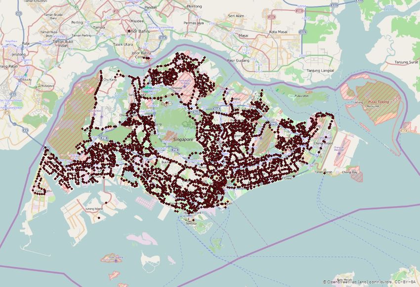
Over 81% (or 3.16 million) of the resident population live in Housing Development Board flats
and 56.6% is concentrated in ten planning areas. Figure 2 shows that there are four planning
areas with more than 250,000 residents, namely Bedok, Jurong West, Tampines and
Woodlands, with Bedok leading with 289,750 residents. The five planning areas with the
highest proportion of residents aged 65 years and over are Sungei Kadut, Outram, Downtown
Core, Rochor and Bukit Merah. Newer estates have a higher proportion of younger working
adults.
The Ministry of Manpower (MOM) reports that the average number of working hours
excluding overtime is 46.2 hours per week in 2013, according to MOM survey. Table A1
reports the working hours across different industries. Individuals working in manufacturing and
construction have the highest number of working hours of up to 53 hours a week, while
individuals in the financial and insurance industry work on average of 41 hours.
92.2 Household Interviews for Travel (HIT) Survey
The first dataset we use is the Household Interviews for Travel Survey, which collects activity
and mobility data for a typical weekday for an individual. A local subcontractor conducts face-
to-face interviews of participants. HIT interviewees are required to provide at least 14 days of
collected data, of which at least 5 have to be validated in order to receive a monetary incentive.
More importantly, interviewees provide household and individual information (such as: postal
code, X-Y coordinates of dwelling building, dwelling type, ethnicity, family size, age,
citizenship, residency type, employment status, occupation type and industry, and personal
income) as well as their means of transport, time, length and purpose of travel, but not the time
spent at the purpose destination. The survey is reported at the individual-block level across
Singapore. The individuals interviewed are randomly selected to be fully representative of the
population mix in each block.
Below, we present the preliminary statistics of the social demographics of Singapore based on
the 2012 HIT survey. We will use these area characteristics later in the analysis to explore the
cross-sectional differences in the labor elasticity to commute time. Tables A2-A4 in the
Appendix report the racial, occupation and citizenship distribution across different planning
areas.
Table A2 shows the racial distribution of Chinese, Indians, Malay and other ethnic groups by
planned area in Singapore. For each township, we calculate the proportion of respondents from
a particular race out of the total number of survey respondents in the township. Figure 2
provides a map of the townships in Singapore. The townships with the highest Chinese
population (over 90%) are Bukit Timah and Singapore River. Geylang and Woodlands are
towns with the highest Malay population (over 20%). Geylang has traditionally been where
most Malays reside for cultural and historical reasons and Woodlands is located near to
Malaysia. Other, which is mainly white-collar expats, are mostly based in Newton, Downtown,
River Valley and Tanglin. The variations in ethnic composition across different township allow
us to identify the effect of cultural differences on the work-travel relation.
Table A3 shows the occupation distribution and variations across townships. The survey
categorizes respondents into 10 groups: 1) Legislator, senior official & manager, 2)
Professional, 3) Associate professional & technician, 4) Clerical worker, 5) Service & sales
worker, 6) Agriculture & fishery worker, 7) Production craftsman & related worker, 8) Plant &
machine operator & assembler, 9) Cleaner, laborer & related worker, and 10) Armed forces
10personnel. This breakdown allows us to relate the type of individuals that substitute travel and
working time. The majority of Singaporeans classify themselves as either professionals or
service and sales workers. Newton, River Valley, Singapore River and Tanglin have the largest
percentage of residents working as professionals. These townships on average have more
white-collar expats with some of the highest income.
Table A4 shows the distribution of different types of citizenships across Singapore. The survey
distinguishes between Singaporean citizens, permanent residents, and others. Others are then
categorized in 7 groups: Employment Pass (highly skilled migrants), S Pass (mid-level skilled
staff earning more than $2,200 a month), Work Permit (low-skilled necessity based from
approved source country in determined employment areas), Work Permit (Foreign Domestic
Workers), Dependent’s Pass, Long Term Visit Pass, and Student Pass. There is large cross-
sectional variation in citizenship. The highest proportion of Singaporean citizens is in Bishan,
Hougang, Rochor and Toa Payoh, the first urbanized areas of the country. In contrast, the
highest proportion of employment pass workers is in Downtown, River Valley, Singapore
River and Tanglin, mostly white collar expat workers. This result is corroborated by the finding
that some of the highest proportions of dependent passes and foreign domestic workers are
found in these areas as well. More importantly, the substantial variations in ethnicity,
occupation and citizenship allow us to understand how different cultural and labor
characteristics are related to the elasticity of market time to travel time.
3. Data and Preliminary results
3.1 Survey Data
We start our analysis with the HIT survey data related to travel destinations and travel times.
Table 1 provides the distribution of the purpose of travel of survey participants. Most travel,
26%, is related to commuting (i.e. travel to go to work) in Singapore in 2012, which is similar
to the US and UK. The proportion of travel time spent on commuting to work has increased by
3% from 2008.
Table 2 presents the use of different modes of transport between 2008 and 2012 for the
working population across different income groups.9 65% of all travel is done by public
transport, up from 58% in 2008, while 21% is done by car or taxi, down from 27% in 2008.
9
The inference does not change if one uses the whole survey population. 62.6% of the population used public
transport in 2012 (60% bus and the rest MRT and LRT) and 54% in 2004 (66% bus and the rest MRT and LRT).
11More than 60% of individuals earning less than 7,000 SGD used public transport in 2012,
which represents over 80% of the Singaporean population. Use of public transport is also
popular among the top income earners, with more than 37% using public transport in 2012 up
from 21% in 2008. This distribution implies that public transport and EZ-Link cards are used
by the whole cross-section of society to a large extent, and public transport data provides a
good coverage of the working population.
Table 3 shows that commute time by car has increased steadily from 21 minutes in 2004 to 26
minutes in 2012, a 24% increase. The commute time of all other means of private transport:
motorcycle, van, shuttle bus, and taxi, has also increased substantially from 2004 to 2012. The
only exception is public transport, where the commute times by bus, MRT and LRT, have
either remained the same or just slightly increased from 2004 to 2012. This is not surprising as
the Singapore government has steadily increased the resources invested in public transport and
has increased the number of MRT stations by introducing two new lines in 2009 and 2014
covering an extra 56 kilometers of rail (the whole length of the country).
More importantly, Table 3 shows that the reported travel time of passengers in cars, vans and
motorcycles is consistently lower than that of the drivers of the vehicle, by a minimum of 8%
and a maximum of 40%. This result is quite surprising as the two commuters (driver and
passenger) are from the same household and depart from the same location at the same time. In
order to control for other heterogeneous effects, i.e. the result being driven by individual
characteristics, we investigate the bias across different household characteristics in Table A5.
The results show that the recollection bias is large, positive, and highly statistically significant
for almost all subgroups, with very few exceptions in categories with few observations. This
implies that there is considerable recollection bias or different perception of time spent on the
road depending on whether one is actively involved in driving or not.
3.2 EZ-Link Card Sample
Our sample data provides all the travel by public transport at the individual level, in Singapore
with individual card ID, for the period August-October 2013. The individual card ID facilitates
the tracking of the traveling, working and leisure patterns of every individual at all times across
our sample period, as long as they commute by public transport. The data provides individual
characteristics of the commuters, because each EZ-link card also serves as a supplementary
identification and concession card for students of recognized educational institutes and citizens
12above sixty years old.10 LTA classifies the passenger types into: adults, children/students and
senior citizens. This classification allows us to more accurately identify the commuting
working adults.
The data also reports 1) the mode of transport (bus, LRT and MRT), 2) the service number of
the transport (bus, LRT and MRT service number and vehicle registration number), 3) the
boarding and alighting station numbers, and 4) the ride start and end date, time and distance
of every ride for all commuters. All bus stops in Singapore have a B+5 digit code. The first
four digits of the bus stop code identify the location of the bus stop. The last digit is used to
differentiate the direction of the service. If the bus stop code ends with ‘1’ for a service
traveling from location A to B, the pairing of this bus stop across the street will have a bus stop
code ending with ‘9’.
This information allows us to track the location and commute of every individual across time.
It facilitates a very accurate measurement of travel time and the likely location of an
individual’s home and workplace. For example, the most frequent stop, the first boarding and
last alighting stop of the day is most likely to be the home stop of an individual. It also allows
one to accurately identify the work place of a full-time working adult that commutes by public
transport to the same work location and back home every day. The duration of each ride allows
us to study the delay, due to traffic congestion or MRT breakdowns, hence exogenous shock to
travel time within individual, while traveling to work.
The data includes all the rides that an individual makes during the day organized by ride ID.
The data also aggregates these rides into a journey with any combination of bus, LRT and
MRT with a journey ID. The journey ID is part of the Distance Fare scheme for a more
integrated fare structure, which ensures that commuters can make transfers (from bus to
MRT/LRT and vice versa) without incurring additional costs. A single journey includes up to
five transfers with a maximum of 45 minutes per transfer. One can take up to two hours to
complete a journey, with a limitation that one’s current public transport service number must
not be the same number as the preceding service number. One can only enter and exit the
MRT/LRT network once in a journey. Otherwise, it is considered a new journey for a
commuter, which is more costly. This information is important in measuring a commuter’s
10
Students and senior citizens are carefully checked for status during the issue and purchase of the EZ-Link card.
There are regular conductors and ticket inspectors at all MRT stations and bus routes to ensure against misuse of
concession cards. Any offender is subject to jail terms or fines of $540 or $750 SGD. Media, Netizens, and
newspapers often publicly shame perpetrators, so that they do not regress to committing the offence again.
13travel time to work without being affected by the number of required transfers to their
destinations.
We supplement the travel data with Geographic Information Systems (GIS) data, which
includes all postal codes in Singapore. Since 1995, a postal code in Singapore consists of 6
digits. The first two digits are the sector code and the last four digits represent a delivery point
within the sector, which allows one to accurately pinpoint living and working locations. For
example: Block 335 Smith Street with the postal code 050335 means the building is located in
sector 05, as classified by the Urban Authority of Singapore, and the last digit 335 represents
the block number 335.
Public and private residential, commercial and industrial buildings are assigned different postal
codes in Singapore. Thus, we have information on whether a bus, LRT or MRT stop is located
near a residential, commercial or industrial building. We use this information to create a
dummy variable equal to one if the work stop is located near an industrial building and zero
otherwise. This dummy variable allows us to differentiate between manufacturing and service
jobs. To proxy for the cultural and labor characteristics of individual commuters, we match
every bus stop/LRT/MRT (hereby bus stop) to a postal code in the HIT data. The furthest
distance of a bus stop from a HIT block is 2 kilometers while the shortest distance is 10
meters.11 Finally, we use weather station data to gather information on heavy rain mornings and
afternoons. Singapore has 66 weather stations (manned and automatic) scattered across the
country, which provide and disseminate information at 30 minute intervals. We use the XY co-
ordinates of the boarding bus stop to determine the closest weather station and collect
information on the weather conditions around the travel time of the individual from home in
the morning and from work in the afternoon.
3.2 Measuring Travel and Market Time
To measure travel time to work and market time at work, we first identify the home location for
each individual. We do this in two ways: a) we calculate the most frequented destination (start
or end) per individual, and b) the starting point of the first travel of the day and the last
destination at the end of the day. Home is defined as the station where a commuter starts for 25
or more days across the sample. We then identify the work location for adults. This is
11
The distance between a bus stop and the HIT block is dictated by the population density of each area.
14computed in two ways: a) the second most frequented destination per individual, and/or b) the
final destination of the first trip of the day and the beginning of the journey after a long break
from travel time. Workplace is defined only when a commuter uses public transport for
arriving and leaving the workplace on the same day with a minimum frequency of 25 times
across the sample. The rest of the destinations are other activities.12
With this classification, we define travel time to work as the duration of a journey from home
station to workplace station in a day. We define market time as the duration between the time a
commuter arrives to the work place station and the time the commuter boards a public transport
from the workplace station or the opposite station.13 This measure might overestimate working
time, as individuals might not use all the time at work to carry out work, however the same
issue arises with survey analysis. However, studies based on time-use surveys also do not
account for the different activities, unrelated to the job, performed while being on the job.
There is some data on such activities in the American Time Use Survey, but it has only recently
been used by Burda, Genadek and Hamermesh (2016, 2017) to understand cross-sectional
differences in activities carried out when not working at work.
By Singapore’s labor law, a full-time worker is one that works at least 35 hours a week. We use
only individuals for whom we can identify a home and a workplace and that travel at least 25
times during the sample period. This leads to a sample of over 652,000 travelers. We conduct
robustness analysis for travelers that go to work for more than 30 days and 40 days over the
sample period.
4. Results
4.1 Commuting and Market Time Statistics
Table 4 presents the basic statistics of individual trips for the whole population. There are about
517 million individual-trip observations in the sample, out of which 410 million are adults, 54
million are children and 52 million are senior citizens. 61.6% of the trips are done by bus and
38.4% by MRT/LRT. The proportion of bus trips is very close to that reported by the HIT
survey in 2012, as reported in the previous section. Therefore, the survey data is representative
12
We report results using the first way of classifying home and work locations, however the results remain
quantitatively unchanged when using the second classification methods. Results are available from the authors
upon request.
13
The last digit of each bus station number is either 9 or 1. If it ends with ‘1’ for a service traveling from location
A to B, the pairing of this bus stop across the street will have a bus stop code ending with ‘9’.
15of travel means used by the public, i.e. there is no bias in recollecting information on the mean
of transport.
We classify work and home stations as described in section 3.2. We retain only adults that
travel daily to and from a classified ‘work station’ for at least 25 days in the sample, for a
sample of 29 million individual-trip observations. There are 652,936 working adults in our
sample.
Table 5 shows that Singaporeans work on average 10 hours. For a five-day working week, we
estimate that individuals in our sample work for 50 hours, which is slightly higher than the
average working time reported by the Ministry of Manpower in Table A1 in the appendix. For
comparison, in the US, the average employed adult works 8.46 hours including travel time to
work, and men (8.95) work on average 1 hour more than women (7.86).
A working adult travels on average about 30 minutes to their work location, and the standard
deviation of travel time is 17 minutes, about 57% of the travel time. Therefore, there is
substantial cross-sectional and time-series variation in travel time despite the short travel
distances in Singapore. The average commute time from the EZ-Link data is 35% higher than
the average public transport time recorded from the survey data. Survey data appears to suffer
from strong recollection bias and severely underestimates travel time for passengers, as also
shown in the discrepancy between driver and passenger travel time recollection. Finally, we
also report the average income based on merged EZ-Link and 2012 HIT data at the block level.
The average income of the working adults in our data is 3,334 SGD a month, which is
comparable to the average Singaporean income of 3,480 in 2012 as reported by the Ministry of
Manpower. Therefore, the traveling sample is highly representative of the country’s working
population.
One concern might be that there is no variation in working and travel time across different
townships, as individuals optimize their housing and commute decisions. Table 6 shows the
distribution of passengers in our sample across Singapore and the mean and median of market
and travel time in different townships with more than 100 travelers. There is substantial cross-
township variation both in market and travel time. The minimum average (median) market time
among townships is 9.0 (9.7) hours and the maximum average is 11.2 (11.4) hours. The
minimum occurs in Central Water and the maximum in Sungei Kadut.
164.2 Extensive Margin
The first step in our analysis is to understand when individuals chose to supply labor, extensive
margin. There are several issues that affect how and when individuals go to work. The first is
the effect of heavy rain in the morning, which might cause travel delays and disruption. On
such days, individuals may choose to work from home (not go to work), they may choose to
drive or take a taxi, which will show up as a non-working day in our sample. Second,
individuals might work less than five days a week and work longer on days that they go to
work.
Table 8 presents the results for the extensive margin analysis from fixed effects panel linear
probability model. The dependent variable is equal to 1 when an individual goes to work during
the working week as per our definition, and zero otherwise. To investigate the rain related
absenteeism, we include several proxies for rain related impediments at the beginning of the
day. We use hourly data from all weather stations in Singapore, between 7 and 9 AM. We then
match each individual’s boarding station to his/her closest weather station. We calculate the
average and maximum rain duration and rain amount every morning. We include a dummy
variable on whether individuals in the household own a car, to proxy for the substitution effect
between car and public transport. This information comes from the HIT survey and is only
available at the block level. We also control for other effects like travel distance, whether the
mean of transport is a bus, and the average travel time. We use day of the week fixed effects to
capture the choice of working from home on certain days or parental leave days, therefore
exclude time fixed effects. Columns (1) and (2) show results with individual fixed effects,
which are dropped in columns (3) and (4), when we introduce individual invariant effects like
vehicle available and average travel time. Standard errors are double-clustered at the individual
and travel day level, see Cameron, Gelbach and Miller (2011).
We find that neither the average nor the maximum rain amount in the morning affects the
decision to work. Longer rain duration decreases the propensity to go to work, on the margin.
However, the propensity to commute to work actually increases with the availability of a
private car. This is probably because one can choose to be picked up by car if the rain persists
throughout the day. It is worth noting that individuals that tend to commute for a longer time as
well as individuals that commute by bus have a lower propensity to go to work.
We investigate the day of the week effect by including day of the week dummy variables in all
our specifications, where the baseline day is Monday. The results show that there isn’t that
much of a difference in the propensity to go to work between the different days of the week and
17this effect holds regardless of the inclusion of individual fixed effects. Individuals appear to
have a slightly lower propensity (6%) to work on Fridays. Overall, the results in Table 7 show
that the choice of going to work mainly depends on the travel distance and on traveling by bus,
rather than rain or day of the week.
4.3 Intensive Margin
Next we turn to the analysis of the relation between commuting time and working time, i.e.
when one does go to work, how much to do they work, conditional on travel time. Economic
theory suggests that individuals account for commuting time as part of their work time. As a
result, individuals will spend less time at work if their commuting time increases. Thus, we
form our null hypothesis as follows:
H1: Commuting time is negatively correlated to market time.
We test this hypothesis by regressing travel time on market time controlling for unobserved
individual fixed effects, time fixed effects, time of travel, and weather. Table 6 reports different
specifications of the panel regression of travel time on market time, with individual and time
fixed effects. Column 1 of Table 7 shows the simple regression of travel time on market time
with individual and time fixed effects. For every minute increase in travel time, an individual
works an additional 44 seconds. The exogenous variation in the duration of each ride, i.e. delay
due to traffic congestion or MRT breakdowns, hence exogenous shock to travel time within
individual, while traveling to work allows us to interpret this coefficient as a causal one. The
result is surprising and is contrary to the negative or insignificant relation suggested by
economic theory, as one expects travel time to either be independent from or negatively
correlated (substitute of) to market time. In other words, an individual should not work an
additional 22 minutes over her 8 hour regular working time, just because she spends an
additional 30 minutes over her average time travelling to work. This result suggests a paradox
in the positive relation between commuting time and market time.
There can be a few mechanical explanations for the positive coefficient. Individuals who travel
earlier or later in the day have shorter trips, because the roads are less congested. Alternatively,
the commute time is more likely to be shorter during peak hours, because of the higher
frequency of public transport during that time. “Start early” is a dummy variable indicating
when an individual starts work 30 minutes before her average starting time. “Start late” is a
18dummy variable indicating when an individual starts work 30 minutes after her average starting
time. “Peak Hour” is a dummy variable that indicates when a trip starts during peak hours (7-9
am). Travel*Start Early, Travel*Start Late and Travel*Peak Hour are interaction terms of
travel time and the start of travel.
Results in Columns (2)-(4) show that individuals who start work early, work longer hours
(quarter of an hour) than their average on the days they start work early. The impact of longer
travel time on their working time is also larger. The interaction term between early start and
travel time is positive and statistically significant. Individuals who start work late work
substantially less than their average on days when they are late. However, a longer travel time
for late starting individuals is not related to working time. Individuals that travel during peak
hours also work on average longer (12 minutes) than those not travelling at peak hours.
Travelling during peak hours has a slightly smaller positive relation to work time.
One potential explanation for our results is that days on which one travels longer are bad
weather days. Large amounts of rainfall may lead to longer bus journeys or more people taking
public transport. In addition, persistent rain might cause people to wait it out at the end of the
working day rather than trying to get to the station in the rain, making it look like they are
working longer. We create a heavy rain dummy variable for the starting station at the beginning
and at the end of the working day. Here we exploit the information we have on the location of
each individual across different times of the day, which we link to national weather service data
for the nearest weather station. We use hourly data from all weather stations in Singapore. We
classify a commute as affected by heavy rain “Heavy Rain” dummy equal to one, when there is
7mm of rain in an hour in the location of the commute (home or work) at the time of the
commute. The U.S. Geological Survey in the U.S. Department of the Interior defines heavy
rain as greater than 4 mm per hour, but less than 8 mm per hour. 14 We classify the destination
of the commute as affected by heavy rain “Heavy at Alight” dummy equal to one, when there is
7mm of rain in an hour in the destination of the commute (home or work) at the time of
alighting. Results in column (5) show that heavy rain seems to decrease working time on
average, i.e. people leave work earlier when they expect heavy rain to occur. Also, heavy rain
attenuates the effect of early and late start. Heavy rain does not seem to have any impact on the
effect of travel time on working time.
14
The average daily rainfall in June, July and August in Singapore is 6mm a day. 7mm of rain in an hour is the
whole day’s rainfall in one hour, therefore very large.
19Finally, we control the previous day’s working time. There is positive inertia in work, where if
one worked long hours one day she will work long hours the next day.15
In summary, we find that market time is positively associated with travel time, contrary to what
economic theory assumes. This paradox is not explained by whether an individual starts her
work early for the day, peak hour effect, and the weather condition during the commute. Our
findings have important implication for the common assumption in economics that travel time
is of part market time and they are negatively correlated.
4.4 Time-series Variation of Delay
From the analysis in Table 8, there appears to be some time-series variation in the effect of
travel time on working time, depending on how early or late an individual starts work.
Individuals starting early seem to have some expediency of getting to work, while those that
are delayed do not seem to worry much about their delay. We investigate this variation in effect
further with two extra pieces of analysis. First, we try to break down the early and late start in
different subcategories ranging from less than 15 minutes to more than one hour. Second, we
investigate repeat delayed arrivals.
Table 9 presents the analysis for different early and late start time. In this regression we control
for relevant variables from the previous analysis: lag dependent variable, peak hour, travel
time*peak hour, industry dummy and travel time*industry dummy and include both time and
individual fixed effects. We start the analysis with early arrivals, those that appear to have
some expediency to get to work. Column (1) shows that there is considerable increase in the
elasticity of work time to travel time, when an individual starts work less than 30 minutes early
and more than 30 minutes early. The interaction term increases form 0.12 to 0.65, i.e. an
individual that gets to work more than 30 minutes early increases working time by 1:49
minutes for each minute of travel delay. In column (2), we break down the less than 30 minutes
early start into less than 15 minutes and between 15 and 30 minutes early. The result shows a
hierarchy of increases in elasticity from 0.05 for 15 minutes early to 0.70 for more than 30
minutes early. Column (3) investigates the same coefficients, but for times when an individual
starts work more than one hour early than their average time. An individual starting one hour
earlier than usual, works 2 more minutes for every minute of travel delay. Finally, column (4)
breaks down the pre- and post-30 minutes early start in 60 minute
15
The results remain qualitatively similar when including only individual fixed effects, so that we allow for
common shocks to public transport in a particular day. Results are available from the authors upon demand.
20You can also read