COVID-19 Impact on Global Maritime Mobility
←
→
Page content transcription
If your browser does not render page correctly, please read the page content below
COVID-19 Impact on Global Maritime Mobility
                                          Leonardo M. Millefiori1,+ , Paolo Braca1,+,* , Dimitris Zissis2,3 , Giannis Spiliopoulos3 ,
                                          Stefano Marano4 , Peter K. Willett5 , and Sandro Carniel1
                                          1 NATO  STO Centre for Maritime Research and Experimentation, Research Department, La Spezia, 19126, Italy
                                          2 University of the Aegean, Department of Product and Systems Design Engineering, Syros, 84100, Greece
                                          3 MarineTraffic, Athens, 115 25, Greece
                                          4 University of Salerno, Dipartimento di Ingegneria dell’Informazione ed Elettrica e Matematica Applicata (DIEM),

                                          Fisciano (SA), 84084, Italy
                                          4 University of Connecticut, Department of Electrical and Computer Engineering, Storrs, 06269, USA
arXiv:2009.06960v3 [econ.GN] 4 Mar 2021

                                          * paolo.braca@cmre.nato.int
                                          + these authors contributed equally to this work

                                          ABSTRACT

                                          To prevent the outbreak of the Coronavirus disease (COVID-19), many countries around the world went into lockdown and
                                          imposed unprecedented containment measures. These restrictions progressively produced changes to social behavior and
                                          global mobility patterns, evidently disrupting social and economic activities. Here, using maritime traffic data collected via a
                                          global network of Automatic Identification System (AIS) receivers, we analyze the effects that the COVID-19 pandemic and
                                          containment measures had on the shipping industry, which accounts alone for more than 80 % of the world trade. We rely on
                                          multiple data-driven maritime mobility indexes to quantitatively assess ship mobility in a given unit of time. The mobility analysis
                                          here presented has a worldwide extent and is based on the computation of: Cumulative Navigated Miles (CNM) of all ships
                                          reporting their position and navigational status via AIS, number of active and idle ships, and fleet average speed. To highlight
                                          significant changes in shipping routes and operational patterns, we also compute and compare global and local vessel density
                                          maps. We compare 2020 mobility levels to those of previous years assuming that an unchanged growth rate would have
                                          been achieved, if not for COVID-19. Following the outbreak, we find an unprecedented drop in maritime mobility, across all
                                          categories of commercial shipping. With few exceptions, a generally reduced activity is observable from March to June, when
                                          the most severe restrictions were in force. We quantify a variation of mobility between −5.62 % and −13.77 % for container
                                          ships, between +2.28 % and −3.32 % for dry bulk, between −0.22 % and −9.27 % for wet bulk, and between −19.57 % and
                                          −42.77 % for passenger traffic. The presented study is unprecedented for the uniqueness and completeness of the employed
                                          AIS dataset, which comprises a trillion AIS messages broadcast worldwide by 50 000 ships, a figure that closely parallels the
                                          documented size of the world merchant fleet.

                                          Introduction
                                          The coronavirus (COVID-19) pandemic has recently produced one of the worst global crises since World War II. As of
                                          January 15, 2021, almost 100 million people have been infected worldwide, and over 2 million have passed away due to the
                                          disease. Consequences of the outbreak are impacting broadly all aspects of our society. In February 2020, the World Health
                                          Organization (WHO) recommended containment and suppression measures to slow down the spread of the virus.1, 2 Towards
                                          this direction and aimed at “flattening the curve” of infections so as to avoid overwhelming healthcare systems, many countries
                                          implemented unprecedented confinement measures, ranging from bans to travel and social gatherings, to the closure of many
                                          commercial activities. Evidence that the lockdown measures achieved a reduction of the rate of new infections is gradually
                                          appearing in the scientific literature.3, 4
                                              Many of the aforementioned restrictions are in contradistinction to “normal” routines. At a time when we are asked to
                                          come together and support one another in society, we must learn to do so from a distance. But the behavior changes have
                                          been deemed necessary, and some may provide useful insights regarding how we can facilitate transformation toward more
                                          sustainable supply and production.7 The hope is that the macroeconomic system, global supply chains, and international trade
                                          relations will not revert back to “normal” and “business-as-usual,” and will allow the emergence and successful adoption of
                                          new types of economic development and governance models.7
                                              On the other hand, both the outbreak and the restrictions are revealing the fragility of the global economy, sparking fears
                                          of impending economic crisis and recession.8 Social distancing, self-isolation and travel restrictions have led to workforce
                                          reductions across all economic sectors. Schools have closed down, and the demand for commodities and manufactured products
                                          has generally decreased. In contrast, the need for medical supplies has significantly risen. The food industry is also facing
passenger ships
60 Daily price (high/low) 200 7-day moving average
Number of flights 200
175
crude oil WTI price [USD]
number of flights × 1000
40
mileage [nmi × 1000]
150
150
20 125
100 100
0 75
50 50
20
25 2019 7-day avg
40 0 0 2020 7-day avg
Feb Mar Apr May Jun Jul Feb Mar Apr May Jun Jul Jan Feb Mar Apr May Jun Jul
2020 2020
(a) (b) (c)
Figure 1. (a) Crude oil WTI price from January to July 2020. 5 Note the sudden and unprecedented negative price in April
2020. (b) Total number of flights tracked by FlightRadar24 from January to July 2020.6 At the end of March there was an
abrupt decrease of the number of flights (∼ 100 000 units) because of the lockdown restrictions. (c) Daily navigated miles by
passenger ships in 2020 compared with 2019.
increased demand due to panic-buying and stockpiling.8
Overall, world trade is expected to fall by between 13 %
and 32 % in 2020 as the COVID-19 pandemic disrupts nor-
mal economic activity and life globally.11 Business activity
across the eurozone collapsed to a record low in March 2020,
and US industrial production showed the biggest monthly
decline since the end of World War II.12 An example of the
unprecedented financial changes is the price of oil dropping
below zero due to expiry of delivery contracts and limited
storage capacity to receive them, for the first time in history
in April 2020,5, 13 as reported in Fig. 1a. The connection
between the recent spread of COVID-19, oil price volatil-
ity, the stock market, geopolitical risk and economic policy
uncertainty in the US is studied by Sharif et al.14 Guan et
al.15 analyzed the supply-chain effects of a set of idealized
lockdown scenarios, using the latest global trade modeling
framework. Given that lockdowns be necessary, the authors
demonstrate that they best occur early, and be strict and
short in order to minimize overall losses.
Useful insight related to the global supply chain can be
gained by observing the impact of lockdowns on the mo-
bility of goods. Indeed, in today’s increasingly globalized
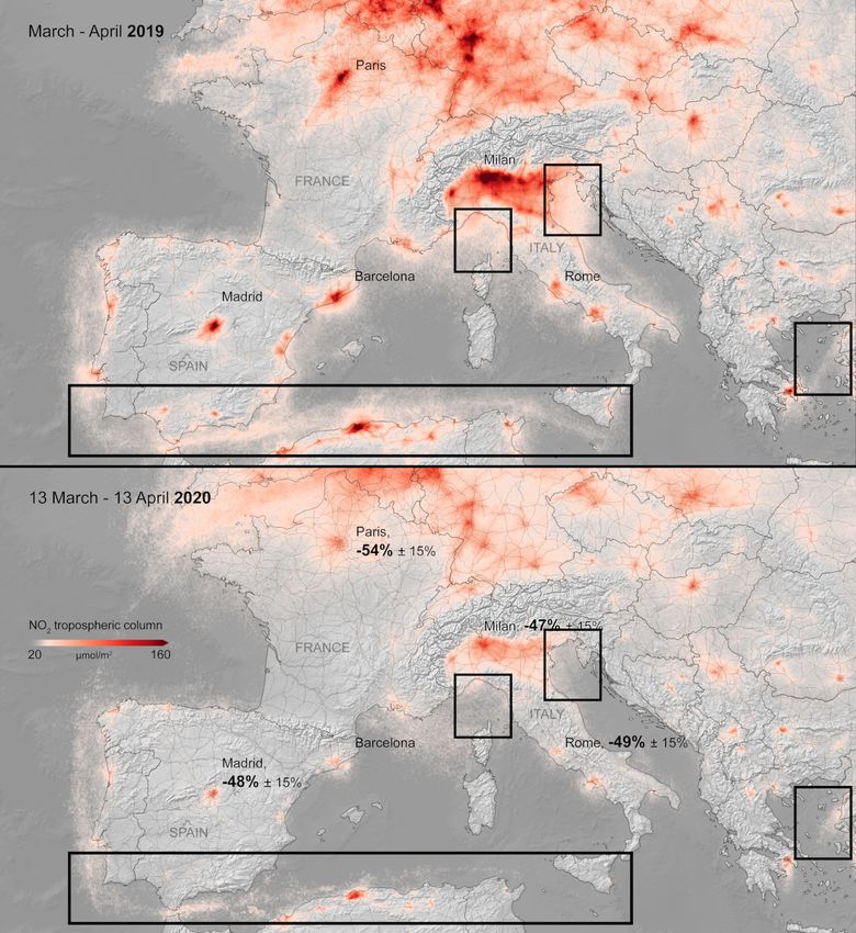
economy, transport plays a central and critical role as the Figure 2. Average nitrogen dioxide (NO2 ) concentrations
primary enabler of the flow of freight within and across from 13 March to 13 April 2020, compared to the same period
borders. In late March 2020, several sources reported a in 2019. The decrease of emission is evident, around −50 % in
dramatic decline in air traffic: as governments put travel re- large European cities (Rome, Paris, Madrid and Milan).
strictions in place, airlines halted flights and commercial air Highlighted with boxes there are regions of sea where it is
traffic quickly dropped significantly below 2019 levels, see evident a decrease of nitrogen dioxide concentrations, probably
Fig. 1b. However, as it accounts only for a small part of the due to the reduced shipping activity. WHO air quality guideline
global freight transport, a decline in air traffic, as significant values quantify in 40 µg m−3 (annual mean) the NO2 limit level
as it may be, would not necessarily imply reduced goods for human health.9 Reproduced with permission. © Contains
mobility. modified Copernicus Sentinel data (2019-20), processed by
With over 80 % of global trade by volume and up to KNMI/ESA.10
70 % of its value being carried on board ships and handled
through seaports worldwide, maritime transport for trade and development is of paramount importance.16–18 Shipping can
be viewed as a barometer for the global economic climate. According to the United Nations Conference on Trade and
Development (UNCTAD), in 2018 total volumes are estimated to have reached 11 billion tons, an all-time high.19 UNCTAD
originally projected an annual average growth rate of 3.4 % for the period 2019—2024.19 However, this estimated growth
2/22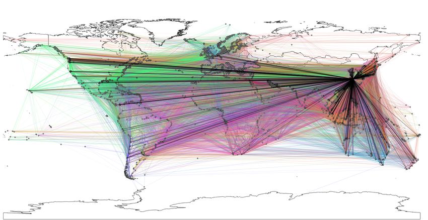
will possibly need to be revised,11 as the coronavirus pandemic led to a 3 % drop in global trade values in the first quarter
of 2020. The downturn is expected to accelerate in the second quarter, according to UNCTAD forecasts,20 which project a
quarter-on-quarter decline of 27 %. For the full year, UNCTAD expects a drop of 20 %. The World Bank further noted that
merchandise trade appeared to have bottomed out in April, falling nearly 20 % year over year, after a 10 % decline in March.
The trade contraction caused by COVID-19 is deeper than the one observed during the financial crisis of 2008-2009.21
     Similar to commercial aviation, the maritime tourism industry was the first and most-affected traffic segment, with cases of
COVID-19 among cruise ships passengers and crew members reported all around the world, from Yokohama (Japan), to Corfu
(Greece) and Sydney (Australia).22, 23 The effects on this market segment might also be more enduring than in other sectors, as
psychological effects might come into play in addition to restrictive measures, with passengers being less inclined to travel on
large crowded ships. In the second half of March 2020, most European cruise terminals partially or in some cases completely
suspended operations23 (e.g., 19 March in Italy, 20 March in Croatia, 25 March in Spain). In order to limit and slow the spread
of the infection, many seaports closed down, limiting—and sometimes banning—cruise traffic at their terminals. National and
local restrictions concerning ship operations were enforced, often leading to delayed port clearance. Limitations included crew
embarking and disembarking, cargo discharge and loading, imposition of quarantine, and eventually refusal of port entry and
refueling. Other measures followed in other maritime sectors and port activities with the aim to ensure safety at terminals and
associated logistic facilities of stevedores and other personnel.24 The fishing and aquaculture sectors were also affected by
containment measures, leading to, e.g., voluntary fishing cessation and suspension or reduction of fish farming, with evident
effects on the supply chain of fish food products.24
     Global maritime mobility reductions not only affect global trade and the economy, but also the environment: especially sea
pollution25, 26 and incursions by invasive species27 are heavily influenced by ship activities; in a recent International Maritime
Organization (IMO) report28 that has been submitted to the Marine Environment Protection Committee (MEPC), greenhouse
gas (GHG) emissions from shipping—expressed in carbon dioxide equivalent (CO2 e)—increased increased 9.6 % in 2018
with respect to 2012, and accounted for the 2.89 % of global anthropogenic emissions, with container and bulk shipping being
accountable for most of the total emissions. The nexus between COVID-19 and the environment already attracted enormous
attention within the scientific community, and several works are already available that analyze the effects of the pandemic in
four main areas:29 (1) environmental degradation, (2) air pollution, (3) climate/metrological factors and (4) temperature. An
exemplary environmental consequence of lockdowns is that pollution levels dropped significantly; for instance, greenhouse gas
emissions, nitrogen dioxide, black carbon and water pollution decreased drastically.29 In Fig. 2 we report, using data from the
Copernicus Sentinel-5P satellite,10 the average nitrogen dioxide concentrations in Europe from 13 March to 13 April 2020,
compared with the same period in 2019. The decrease of pollutants is evident, around −50 % in large European cities (Rome,
Paris, Madrid and Milan). In the same figure, we have also highlighted with boxes sea regions where the decrease of nitrogen
dioxide concentrations is noticeable and could be also due (even if only partially) by a decreased shipping activity. Indeed, it
is interesting to observe that just along the first part of one of the main sea lanes in the Mediterranean Sea (Gibraltar-Suez),
pollution in 2020 reduced with respect to 2019 levels. Recent work by Faber et al.30 suggests how emissions from ships
could be reduced if they reduced their speed; our analysis of AIS data shows that in all highlighted areas, on average, ships
reduced their speed in March-April 2020 with respect to the same months in 2019. Specifically, in the highlighted regions of
the Gibraltar-Suez route, Ligurian Sea, Northern Adriatic Sea, and Aegean Sea, we report average fleet speed variations of
−5.1 %, −15.3 %, −6.0 % and −9.5 %, respectively.
     The aim of this study is to analyze the short-term effects that the COVID-19 pandemic and containment measures had on
global shipping mobility. While a reduction of shipping activities is qualitatively expected from several factors, e.g., from
shipbuilders’ reduced capacity and new ship building orders about 75 % down,32 we specifically aim at providing a quantitative
evidence-based assessment of such reduction. For this reason, we opted for purely data-driven indicators that could measure
exhaustively the impact of the lockdown and containment measures on maritime traffic directly, also in ways that could not
have been easily anticipated. The analysis reported in this paper shows the combined effects of the coronavirus disease and the
containment measures, in addition to the reported trade contraction,11, 20, 21 had on the global maritime traffic. Maritime traffic
reflects these effects and as such shows, for the first time and in specific sectors more than others, signs of slowing down, with
possible negative future consequences on the entire global supply chain.
     We propose the spatio-temporal analysis of positional AIS messages to compute synthetic indicators capable of quantifying
ship activities and highlighting changes in mobility patterns. The indicators are the Cumulative Navigated Miles (CNM),
computed for each ship journey per category, the number of active and idle ships and their average speed. To complement
our analysis and highlight significant changes in shipping routes operational patterns, we also compute vessel density maps
and show differences between the density of shipping traffic in 2019 and 2020. In other words, we assess, with a thorough
data-driven approach, the global ship mobility for the traffic categories that account for the most traffic worldwide. As a matter
of fact, the available statistics on maritime trade, or the related economic indicators, are not suitable to quantify exhaustively
changes in shipping mobility patterns.

                                                                                                                             3/22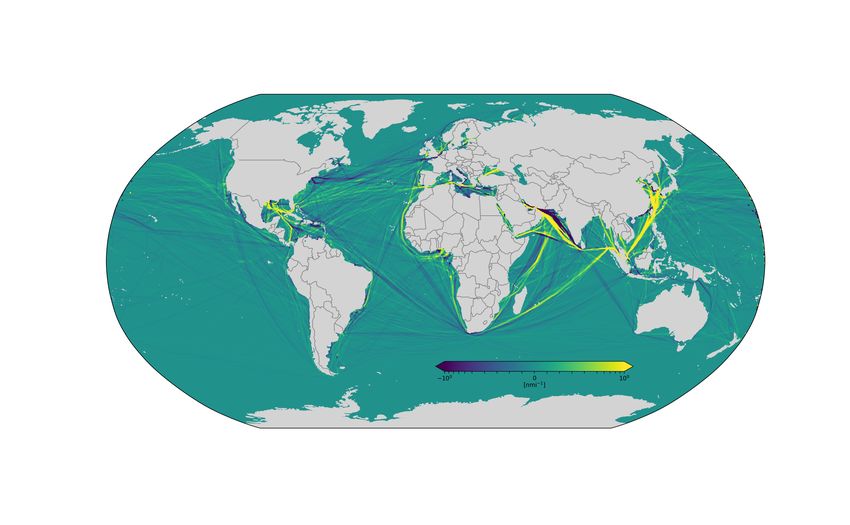
Figure 3. Representation of Shanghai’s ego network and its 3-step neighborhood: each port in the picture, represented by a
circle on the coastline, is reachable from Shanghai with at most three hops. An ego network31 consists of a focal node (the ego)
and the nodes (the alters) that are connected to it, either directly or within a fixed number of steps. The edge color is
representative of the country of the port of origin.

    Indeed, maritime trade statistics,19–21, 33 being focused on measuring the accessibility to global trade more than mobility
patterns, are generally based on connectivity indexes, such as UNCTAD’s Liner Shipping Connectivity Index (LSCI), and
calculated at the country level. On the other hand, economic indicators, such as the Baltic Dry Index (BDI), are meant to
provide an assessment of freight cost on various (selected) routes. Even if they are both driven by the shipping mobility, none
of them is actually suitable to assess the mobility of vessels globally. Given today’s ubiquity of AIS, both maritime trade and
economic indexes are computed also with the support of AIS; however, the aim is to measure different entities than shipping
mobility, and they cannot be computed from AIS alone. For instance, one of the components of the LSCI is the number of
scheduled port calls, or Port Visits (PVs), which can be computed automatically from AIS data. However, the automatic
computation of PVs from AIS data may cause inaccuracy. As an example, the PVs may not get recorded because of low AIS
coverage (or because the AIS device is switched off), or because the visited port is too small to appear in the ports’ database.
Care needs to be taken to ensure that all PVs are captured in the data, and that all PVs relate to actual operations and not, for
instance, maintenance in a shipyard or refueling. It is noteworthy to mention Singapore, which will often appear as a destination
for bulk carriers, even though there are no dry bulk terminals in the city state.
    Given such limitations of AIS-derived PVs, which focus only on the end points of a voyage, we propose data-driven
indicators that can look at a complete voyage and do not introduce additional “uncertainty” in the related calculations. Indeed,
the CNM indicator (which is highly correlated to PVs, as we show in the Methods section) does not suffer from such limitations,
as the ship trajectory can almost always be reconstructed in the data processing phase, even if pieces of it are missing.
    Moreover, it is intuitive to acknowledge that there is a close relationship between mobility (e.g., the number of active or
idle ships) and trade volumes; as such, shipping mobility, too, can be understood as a proxy for economic activity. Yet, even
today most statistics and economic forecasting indices focus only on the starting and finish lines of the supply chain, with little
consideration of how goods arrive at their final destination. A more detailed look reveals a complex and dynamic network of
ships and their cargo in constant motion across the world’s oceans. In this sense, maritime traffic can provide insights into the
global supply and demand trends; thus considered as an indicator of future economic growth.
    The results reported in this paper are based on a global dataset containing approximately a trillion AIS messages collected
between 2016 and 2020 indicating the movement of more than 50 000 commercial ships across the globe, stored in a big data
infrastructure of 55 TB. To give an idea of both the worldwide coverage of AIS data and the capillarity of sea-routes network,
we proffer in Fig. 3 the port of Shanghai’s ego network31 constructed based on AIS data from September 2018–2019.
    The global CNM that we have computed from AIS data indicates the scale of ship mobility. From January to June
ships cumulatively travelled something around around 530 000 000 nautical miles (nmi) in 2016, 580 000 000 nmi in 2019,
and 575 000 000 nmi in 2020. To aid understanding, the distance commercial shipping travelled in the first half of 2016 is
comparable to travelling 6.5 times the mean distance between the Earth and sun, and in 2019 almost 7.2 times that.

                                                                                                                             4/22
Instead of increasing, as has happened in all past years since 2016, the global ship mobility in terms of CNM, in 2020 and
for the first time, slightly decreased. The decrease in the first half of 2020, compared to the first half of 2019, amounted to a
modest 0.9 % and to over 5 % in the period April-June 2020, compared to April-June 2019. The decline in the first half of
2020 is almost 4 %, compared to the forecast values in 2020, and is over 8 % in the period April-June. Moreover, there is great
variation of this figure among traffic categories and different months; for instance, in June container ships decreased 12 %
compared to 2019, wet bulk ships of 5 %, and passenger ships of 42 %, while dry bulk ships slightly increased (1.7 %).

Results
The COVID-19 pandemic has led to vast economic disruption across the world, and industry activity and confidence have
collapsed.12 Overall, the shipping industry and seaborne trade followed this negative trend. In this paper, we compare global
vessel mobility during the first half of 2020 to that of previous years, from 2016 to 2019, and the analysis confirms that shipping
mobility has been negatively affected, but to different degrees in each market and depending on the size of vessels. Our results
suggest that there is a substantial increase in idle ships across all types of ships/markets globally in the first six months of
2020, and a substantial decline in the vessel mobility measured in CNM per unit of time. Given that, prior to the pandemic, the
mobility—similar to global trade—was on an increasing trend, we compare the 2020 mobility with its forecast based on the
analysis of previous years. Specifically, we assume an expected growth in 2020 given by the average growth observed in the
same month of a few past consecutive years.
    We have analyzed variations of shipping operational patterns computing the difference of spatial traffic density in 2019 and
2020, reported in Figures 5, 6, 7 and 9. A quantitative analysis is represented in Fig. 8, which reports global vessel mobility
indicators for four main types of ship traffic: container (a)–(c), dry bulk (d)–(f), wet bulk (g)–(i), and passenger (j)–(l). For
each traffic category, we report the daily navigated miles from January to June in 2019 and 2020, the monthly navigated miles
from 2016 to 2020 (with 2020 forecasts), and the monthly percentage of active/idle ships from 2016 to 2020. The global CNM
values in Fig. 8 are also reported in Table 1 for each category, where we provide all the total aggregate values.
    Interestingly, the mobility forecasts in January and February 2020 (before lockdowns) underestimate the growth of some
markets, such as the container (Fig. 8b), dry bulk (Fig. 8e), and wet bulk (Fig. 8h) markets, in the sense that the actual 2020
levels are between +1.11 % (dry bulk in February) and +5.17 % (wet bulk in February) with respect to the forecast level.
Conversely, the forecast severely overestimates the mobility growth of passenger ships since January, −3.69 % w.r.t. the
expected level, up to a dramatic −45.3% in May, as depicted in Fig. 8k. In general, the analysis reveals an overall decrease of
mobility levels in 2020 compared both with their expected value (considering the growth observed in past years) and to 2019
levels, with only a few exceptions.
    We must note that there is a possible regional effect in
the measured mobility levels; the mobility in specific re-
gions might be impacted more than others. Specific sectors             85
                                                                                                 wet bulk :: vlcc/ulcc
of the shipping industry were more resilient and continued
delivering goods, while others have been much more vul-                80
nerable to such measures (e.g., cruise ships). Indeed, the
essential supply chain, e.g., hospital and food, was guaran-
                                                                       75
                                                                   % active ships

teed when the restriction measures were in place across the
world.
                                                                       70
    Figures 8a–8c show an evident slowdown in the mobil-
ity of container ships with respect to previous years, with an
increase of idle ships and a correspondent decrease of nav-            65

igated miles. The slowdown becomes apparent in March,                         2019 7-day avg
                                                                              2020 7-day avg
in comparison to both 2019 and 2020 forecasts. Global                  60
                                                                          Apr                May                       Jun      Jul
navigated miles of container ships in June 2020 was on aver-
age 10 % below the level in June 2019, and 13.77 % below
the 2020 forecast. Figures 8d–8f inform on the effects of          Figure 4. Daily active and idle ships in 2019 (in blue) and
lockdowns on dry bulk shipping. Overall, there is a small          2020 (in orange) of the supertankers, Very Large Crude
increase in idle ships from January to April, and a decline of     Carrier (VLCC) and Ultra Large Crude Carrier (ULCC). The
the navigated miles in May and June. This market appears           two area charts are overlaid in transparency to highlight trend
to be less sensitive to the implemented containment mea- differences. It is evident a decrease (increase) of active (idle)
sures, at least in the short term. The reason is maybe that        ships for this category from April, 2020, not present in 2019.
dry bulk carriers transport a wide range of cargo, including       This is confirming the use of a significant subset of
goods whose demand increased due to the pandemic, such             supertankers as oil storage.34
as paper pulp, with several ports reporting record quantities.

                                                                                                                             5/22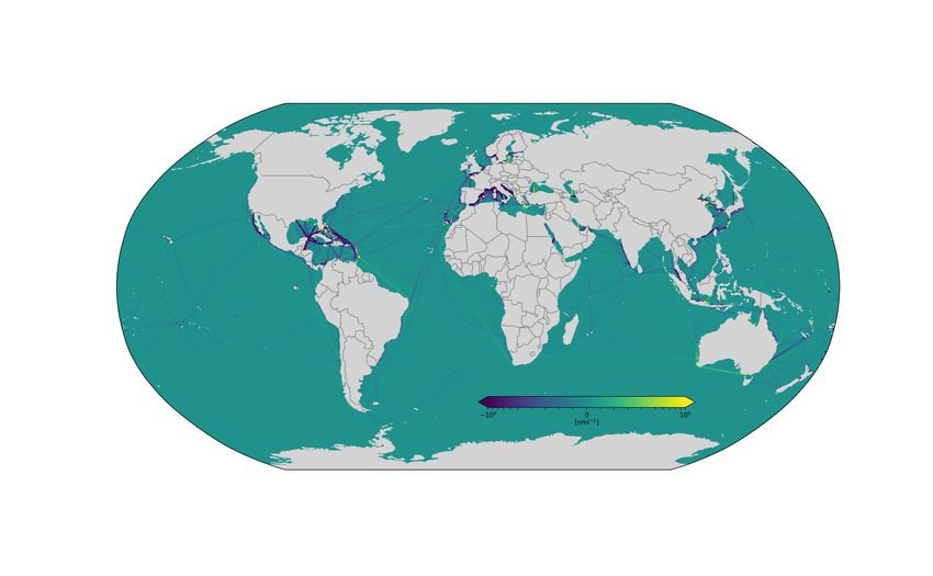
Table 1. Monthly Cumulative Navigated Miles (CNM) [nmi × 106 ].

                       Year         January        February         March            April            May             June
                      2016           23.68           23.45           26.01           25.51           26.42           25.35
                      2017           26.10           23.28           26.82           25.84           26.76           25.16
                      2018           26.17           24.32           26.12           26.10           27.61           26.85
      Container
                      2019           24.96           22.92           25.91           26.08           27.82           27.24
                      2020†          25.39           22.74           25.88           26.27           28.29           27.88
                      2020‡          26.20           23.11           24.43           23.98           24.15           24.04
                      2016           32.67           31.99           37.08           36.94           37.65           35.38
                      2017           38.33           34.43           39.13           38.79           40.25           37.83
                      2018           37.76           36.27           39.90           39.36           41.60           39.29
       Dry bulk
                      2019           37.38           35.69           39.45           39.77           42.82           41.93
                      2020†          38.95           36.92           40.25           40.72           44.55           44.11
                      2020‡          40.32           37.33           41.17           41.17           43.44           42.65
                      2016           21.28           20.92           23.24           22.69           23.26           22.48
                      2017           24.50           21.69           24.99           24.34           25.18           23.84
                      2018           24.55           23.22           25.40           24.84           26.02           24.84
       Wet bulk
                      2019           24.88           23.21           25.94           25.22           27.04           26.28
                      2020†          26.07           23.98           26.84           26.06           28.30           27.55
                      2020‡          26.92           25.22           26.78           25.92           26.18           24.99
                      2016             4.78           4.73            5.32            5.31            5.51            5.57
                      2017             5.33           4.87            5.62            5.67            5.88            5.96
                      2018             5.46           5.06            5.74            5.75            6.00            6.08
      Passenger
                      2019             5.70           5.19            5.91            5.92            6.23            6.25
                      2020†            6.00           5.35            6.11            6.12            6.47            6.48
                      2020‡            5.78           5.32            4.92            3.44            3.54            3.71
                      2016           82.42           81.09           91.64           90.46           92.85           88.78
                      2017           94.26           84.26           96.56           94.64           98.07           92.79
                      2018           93.94           88.88           97.16           96.05          101.22           97.06
           Total      2019           92.91           87.01           97.22           96.99          103.92          101.70
                      2020†          96.41           88.99           99.08           99.17          107.61          106.01
                      2020‡          99.22           90.98           97.29           94.51           97.32           95.39
  †   Forecast mobility levels considering the average growth in past years 2016–2019.
  ‡   Actual mobility levels recorded in 2020.

However, still there is a noticeable decrease, 2.5 % and 3.3 % in May and June, respectively, if compared to the forecast levels.
Figures 8g–8i show the mobility of wet bulk shipping. An evident rise of idle ships from the beginning of the year is apparent
in this category, with a corresponding decrease of navigated miles from February to June. The reduced mobility of this shipping
category is already observable in May and June, if compared with 2019 values, and this being a growing market, the loss is
even more pronounced if compared with the expected mobility levels in 2020, with a loss that can be assessed around 7.5 % in
May and 9.3 % in June. Finally, Figures 8j–8l report on the global mobility of passenger ships, the traffic category that was
most affected by lockdown measures, with a dramatic collapse of monthly mileage recorded since March (more than 40 % less
than what expected by 2020 forecasts) and a corresponding increase of idle vessels.
    For a closer look into each market, we report the daily navigated miles broken down by ship size. In Fig. 11, we compare
the daily navigated miles for container ships according to their capacity. Specific segments show a stronger decline compared
to others. Across all vessel sizes, with the exception of Ultra Large Container Vessels (ULCVs), from late February or early
March, there is a strong decrease of the navigated miles. As before, we must note that, since specific segments and types of
ships operate on specific trade routes and regions, there could be regional effects that, in the global indicators, are “averaged
out”; in other words, local trends could be different than the global one. This is evident from the density map analysis, which
show exactly how changes are spatially distributed. However, if considered globally, the ULCV market declined; ship operators
cancelled their services, with a consequent decrease of both active ships and navigated miles. In Figures 12 and 13, a similar

                                                                                                                             6/22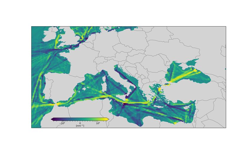
(a) Container

                                                         (b) Dry bulk

Figure 5. Monthly CNM density difference between 2020 and 2019 for container (a) and dry bulk (b) shipping. The
considered time period is from 13 March to 13 April. Each grid cell is colored based on the variation of the 2020 value with
respect to 2019, ranging from dark purple, which represents a decrease of CNM in 2020 with respect to 2019, to bright yellow,
which represents instead an increase of navigated miles in 2020 with respect to the previous year.

                                                                                                                        7/22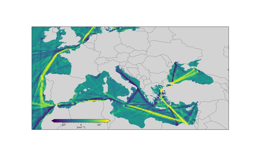
(a) Wet bulk

                                                        (b) Passenger

Figure 6. Monthly CNM density difference between 2020 and 2019 for wet bulk (a) and passenger (b) shipping. The
considered time period is from 13 March to 13 April. Each grid cell is colored based on the variation of the 2020 value with
respect to 2019, ranging from dark purple, which represents a decrease of CNM in 2020 with respect to 2019, to bright yellow,
which represents instead an increase of navigated miles in 2020 with respect to the previous year.

                                                                                                                        8/22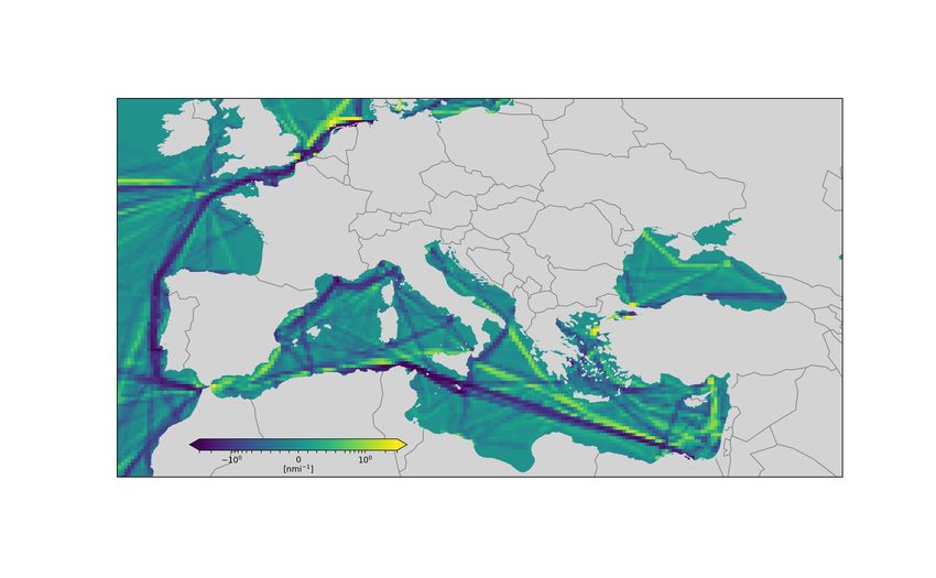
(a) Container                              (b) Dry bulk                              (c) Wet bulk

Figure 7. Monthly CNM density difference in the area around the Suez Canal between 2020 and 2019 for container (a),
dry (b) and wet bulk (c) shipping. The considered time period is from 13 March to 13 April. Each grid cell is colored based on
the variation of the 2020 value with respect to 2019, ranging from dark purple, which represents a decrease of CNM in 2020
with respect to 2019, to bright yellow, which represents an increase of navigated miles in 2020 with respect to the previous year.

analysis is available for dry and wet bulk carriers. Dry bulk shipping refers to the movement of commodities carried in bulk:
iron ore, coal, grain, steel products, lumber and other commodities classified as the minor bulks. For this category, only a
small decrease of mileage across all vessel sizes is observed. In Fig. 13, we report the daily navigated miles for wet bulk
shipping broken down by ship capacity. Wet bulk cargoes include petroleum products, crude oil, vegetable oils, chemicals and
similar products. The slowing demand in goods’ production and oil consumption had an effect on the mobility of all vessel
sizes. The most significantly affected have been the larger tankers, specifically Panamax, Aframax and Suezmax sizes being
affected the most; comprehensive information on ship classification by their size is available to the interested reader in the open
literature.35, 36 Due to circumstances unrelated to COVID-19 (i.e., the breakdown of the OPEC alliance—which triggered a
30 % fall in oil prices in March 2020), the mobility reduction is evident only after April 2020. Finally, Fig. 14 reports the daily
navigated miles of passenger vessels, the most affected segment by lockdown measures. The loss in terms of navigated miles
in 2020 compared to 2019 is apparent, with larger vessel sizes affected by stronger losses than smaller ones. With respect to
2019, passenger ships larger than 60K GT, which includes large cruise ships, registered a sharp decrease of navigated miles of
more than 80 % since March 2020, when several cruise lines, including Carnival cruises, which alone owns more than 100
cruise ships, suspended the operations. The effects are evident from Fig. 14, with a sharp drop of navigated miles apparent
since March.

Analysis of daily average speed
In Figures 15–18, we report the daily average speed broken down by ship size and category. For the container, dry bulk and wet
bulk categories, the average speed did not change significantly from January to June 2020. Instead, passenger ships exhibit a
significant decrease in average speed, as reported in Fig. 18, a behavior that is coherent with the trend of CNM reported in
Fig. 14. Figures 11–13 show an increase of the average speed for several classes of container, dry bulk and wet bulk in May and
June 2019, which is not observed in 2020. Again, this is coherent with the slowdown of the CNM in 2020 compared to 2019
for most of ship traffic, except dry bulk traffic, as reported in Figures 11–13.
    The mobility of tanker vessels deserves a dedicated analysis. Several sources reported an increase, up to at least 160 million
barrels, of oil held in floating storage on tanker ships, including 60 supertankers, VLCC and ULCC, which can hold 2 million
barrels each.34 The effects of this trend are noticeable in the decrease of CNM at the beginning of May, reported in Fig. 13f and
in the decrease of active supertankers from April to July, 2020 (not present in 2019), reported in Fig. 4.

Shipping traffic density analysis
Vessel density maps are data products that show the spatial distribution of ships, and hence of maritime traffic, in specific
areas of interest; vessel density maps are widely used to understand shipping operational patterns. There are several ways of
computing vessel density maps from AIS data.37 In this work, the method employed to compute density maps amounts to
summing up the length of all tracklets that intersect each cell of a pre-defined grid over the area of interest.37 The resulting
amount is then divided by the cell’s area in squared nautical miles. The reason of this choice is that the produced maps show the
density of navigated miles; consequently, their unit of measure is nmi−1 . In this way, excluded the possible distortion introduced

                                                                                                                              9/22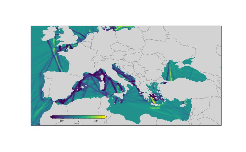
container ships container ships container ships
100
+3.20%
800 25 -5.62% -8.71% -14.61% -13.77%
+1.62%
80
mileage [nmi × 1000]
active/idle ships (%)
mileage [nmi ×106]
600 20
60
15
400
2016 40
10 2017
200 2018
5 2019 20
2019 7-day avg 2020 (exp)
0 2020 7-day avg 2020
0 0
Jan Feb Mar Apr May Jun Jul Jan Feb Mar Apr May Jun Jan Feb Mar Apr May Jun
month month
(a) Container: daily mileage (b) Container: monthly mileage (c) Container: active/idle ships
dry bulk dry bulk dry bulk
1400 -2.48% -3.31% 100
+3.53% +2.28% +1.10%
40 +1.11%
1200
80
mileage [nmi × 1000]
active/idle ships (%)
mileage [nmi ×106]
1000
30
800 60
600 20 2016 40
400 2017
2018
10 2019 20
200
2019 7-day avg 2020 (exp)
0 2020 7-day avg 2020
0 0
Jan Feb Mar Apr May Jun Jul Jan Feb Mar Apr May Jun Jan Feb Mar Apr May Jun
month month
(d) Dry bulk: daily mileage (e) Dry bulk: monthly mileage (f) Dry bulk: active/idle ships
wet bulk wet bulk wet bulk
+3.23% -0.22% 100
-0.54% -7.48%
800 +5.17% -9.27%
25
80
mileage [nmi × 1000]
active/idle ships (%)
mileage [nmi ×106]
600 20
60
15
400
2016 40
10 2017
200 2018
5 2019 20
2019 7-day avg 2020 (exp)
0 2020 7-day avg 2020
0 0
Jan Feb Mar Apr May Jun Jul Jan Feb Mar Apr May Jun Jan Feb Mar Apr May Jun
month month
(g) Wet bulk: daily mileage (h) Wet bulk: monthly mileage (i) Wet bulk: active/idle ships
passenger ships passenger ships passenger ships
100
200 6 -3.69%
-0.49%
5 -19.57% 80
mileage [nmi × 1000]
active/idle ships (%)
mileage [nmi ×106]
150
4 -42.77% 60
-43.75% -45.30%
100 3
2016 40
2017
50 2 2018
2019 20
2019 7-day avg 1 2020 (exp)
0 2020 7-day avg 2020
0 0
Jan Feb Mar Apr May Jun Jul Jan Feb Mar Apr May Jun Jan Feb Mar Apr May Jun
month month
(j) Passenger: daily mileage (k) Passenger: monthly mileage (l) Passenger: active/idle ships
Figure 8. Comparison of traffic indicators for several ship categories: container (a)–(c), dry bulk (d)–(f), wet bulk (g)–(i), and
passenger (j)–(l). The left column shows daily navigated miles in 2019 (in blue) compared with 2020 (in orange); the two area
charts are overlaid in transparency to highlight trend differences; the discontinuity in the blue data series corresponds to the
leap day absence in 2019. The mid column shows monthly navigated since 2016 up to 2020; the second last bar in each group
represents an estimation of navigated miles in 2020 given the growth rate observed in the previous years; the label on the 2020
bar quantifies the percentage increase or decrease w.r.t. the expected 2020 traffic volume. The last column shows the
distribution of active (green) and idle (orange) ships over time, compared with past years, arranged by month with bars from
left (2016) to right (2020); purple bars represent the (negligible) part of ships that could be labeled neither as active nor idle.
by the projection, CNMs can be seen as the double integral of the density over an area of interest. Therefore, to all means, such
density maps provide a complementary perspective on the CNM analysis: while the latter provides a synthetic quantitative
indication of changes induced to maritime traffic, the former shows exactly how these changes are spatially distributed.
In the interest of brevity, we focused this analysis on one month only, from 13 March to 13 April in both 2019 and 2020.
Moreover, instead of just showing the density in two comparable time periods, to highlight changes between one year and the
other, we compute their difference and color each grid cell according to a sequential colormap: if a cell’s value in 2020 is
significantly higher than in 2019, the cell’s color is bright yellow; conversely, if a cell’s value in 2020 is significantly below
2019, its color is dark purple; between these two extremes, cells whose values changed slightly in 2020 with respect to 2019 are
coloured in shadings from blue to green. Consequently, regions with a predominance of dark purple cells represent areas where
vessels generally navigated much less in 2020 than in the previous year; on the other hand, regions where bright yellow are
predominant represent areas with an increase of navigation in 2020 with respect to 2019.
We computed density maps in three areas: worldwide, in the Mediterranean Sea, and in the area around the Suez Canal.
The world density map is illustrated in Figures 5–6. For container shipping, Fig. 5a shows evident signs of reduced activities
10/22(a) Container (b) Dry bulk
(c) Wet bulk (d) Passenger
Figure 9. Monthly CNM density difference in the Mediterranean Sea between 2020 and 2019 for container (a), dry (b), wet
bulk (c) and passenger (d) shipping. The considered time period is from 13 March to 13 April. Each grid cell is colored based
on the variation of the 2020 value with respect to 2019, ranging from dark purple, which represents a decrease of CNM in 2020
with respect to 2019, to bright yellow, which represents an increase of navigated miles in 2020 with respect to the previous year.
along important routes, such as that from the Strait of Malacca to the Mediterranean Sea via the Suez Canal, between North
America and the Strait of Gibraltar, around West Africa and the Iberian Peninsula, just to mention some. Coherently with
Table 1, the analysis of the density of dry and wet bulk vessels, reported in Figures 5b and 6a, reveals instead a general increase
of navigation in some regions, e.g., across the Suez Canal and along the East-West route around the Cape of Good Hope, and a
decrease in other regions, e.g., along several Atlantic routes that connect Europe to North and South America. In general, all
categories of commercial shipping show increased activity in South and East China Seas, evidence of China’s effort to return to
normality sooner than other countries. Coherently with Table 1, the density of passenger ship traffic (Fig. 6b) provides yet
another confirmation that this was the most affected segment by the pandemic, with sharp decrease of shipping activities all
around the globe. The few light increases in activities noticeable in Fig. 6b, e.g., between the Cape of Good Hope and West
Africa or off the coast of South Australia, are explained with the repatriation operations of crew and passenger of cruise ships.38
Suez Canal
The Suez Canal allows fast connections between Europe and the Near and Far East. As such, it has a crucial role for trading,
and deserves a more focused analysis. According to a new market analysis released by BIMCO,39 the overall traffic at the
Suez Canal has remained resilient. Strong increases in the number of transits by oil tankers and dry bulkers helped to offset the
declines in container ship transits according to BIMCO.39 The density maps illustrated in Fig. 7 are in complete agreement
with BIMCO’s analysis and provides further evidence in support of such assessment. Indeed, Figures 7b-7c show an evident
increase of dry and wet bulkers; at the same time, Fig. 7a shows a noticeable decreased activity for container shipping in the
same area. This is mostly a consequence of the increased number of vessels that bypassed the Suez Canal, using instead the
route around the Cape of Good Hope, motivated by low bunker prices and lack of demand in European markets.40 This effect
on the global scale is visible in Fig. 5a.
Mediterranean Sea
The analysis of traffic density differences between 2020 and 2019 in the Mediterranean Sea, reported in Fig. 9, reveals a
situation similar to that already discussed in the area around the Suez Canal. The analysis of AIS data for container shipping
11/22(Fig. 9a) shows a mixed situation, with a prevalent reduction on the western side (Tyrrhenian, Ionian, Adriatic, Ligurian,
Balearic, and Atlantic Seas), considering that lockdowns in Italy, France and Spain happened before than in northern countries,
e.g., Germany. The analysis of the density of dry and wet bulk carriers, reported in Figures 5b and 6a, reveals instead a
general increase of navigation in most of the regions, except for Italy (Tyrrhenian, Ionian, Adriatic and Ligurian Seas), where a
noticeable reduction is observed. The passenger density reported in Fig. 9d, as expected, revels a total collapse of the category
almost everywhere.
Discussion
The COVID-19 pandemic and containment measures have lead to vast economic disruptions across the world, with near
evaporation of both customer demand and industrial activity. Focusing on the first half of 2020 compared with previous years
(2016–2019), and based on a global dataset of approximately 1 trillion ship positions received via AIS from more than 50 000
vessels, the analysis presented in this paper shows that shipping mobility has also been affected negatively.
We report an unprecedented slowdown in global shipping mobility, which was steadily increasing since 2016, and a
noticeable activity decrease for all ship categories in 2020, when compared with projections (assuming the average growth rate
of past years). The most affected traffic segment is that of passenger ships, followed by container ships. Effects of the pandemic
on global ship mobility are observable since March until the end of June 2020, with variations ranging between −5.62 % and
−13.77 % for container ships, between +2.28 % to −3.32 % for dry bulks, between −0.22 % and −9.27 % for wet bulks, and
between −19.57 % and −42.77 % for passenger ships.
On the basis of the indicators presented in this paper, we can also conclude that, despite the crisis, shipping was resilient,
and in specific markets it was possible to continue operations; in this sense, the analysis highlights the strategic importance of
shipping at a global scale. This statement is supported by thorough quantitative analysis of shipping mobility and operational
patterns that shows what happens when the shipping system is subject to an extreme shock, such as that caused by COVID-19
pandemic. The effects of the shock on the system are deep and extend to trade and environmental aspects, even if the exact
nexus between shipping mobility, trade and environmental emissions is still an open research topic. Future works could be
aimed at validating such connections, and explore quantitatively the relation among mobility, trade, and emissions. Additionally,
as more data becomes available our analysis will focus on longer term impacts while attempting to identify signs of a recovery.
Methods
Automatic Identification System (AIS)
Originally designed only for collision avoidance and information exchange between ships, nowadays the AIS is extensively
used by operators as the primary means for ship traffic monitoring on a much larger scale than that achievable with conventional
coastal surveillance systems. With AIS, ships voluntarily broadcast their position, velocity, along with other identification and
voyage-related information. The AIS communication protocol is asynchronous and prescribes that different types of messages
be transmitted with different frequencies. There are two types of AIS transponders: Class A, for large ships, and class B, for
smaller vessels. The International Maritime Organization (IMO) mandates that every ship of more than 300 gross tonnage,
all passenger ships and all fishing vessels with a length above 15 meters be equipped with class A transponders. Conversely,
class B transponders are designed to bring the benefits of AIS on smaller vessels; indeed, they are smaller and less expensive
than class A type transceivers. As such, they can be installed on small ships such as recreational vessels that want to have the
benefits of having the AIS even if, for their size, they are not required to fit a transponder onboard.
Over the last few years, AIS data have been extensively used in research for validation purposes as “ground-truth”
information, e.g., in maritime surveillance with coastal radars41–43 as confirmation tracks for radar detections, or for the
validation of a target motion model for long-term ship prediction.18 AIS has also been used to show how the data association
can be significantly improved using the long-term prediction and combining AIS with HF Surface Wave radar (HFSWR) data,
or Synthetic Aperture Radar (SAR) data.44 But in any case, there is a significant literature that considers AIS the sole source of
information for maritime surveillance,18, 44–48 port traffic analysis,49, 50 and anomaly detection;51–55 a common application for
historical AIS data is also the training of machine learning, including neural networks, algorithms.47, 56, 57 The interested reader
can find in the scientific literature an excellent survey48 of AIS data exploitation for safety, anomaly detection, route estimation,
collision prediction, and path planning.
Data processing pipeline
In this paper, we analyze AIS data to compute mobility indicators. Besides AIS, we made use of information regarding ship
characteristics; such as their class, size and type of cargo (i.e., dry or wet bulk), as well as their weight and referred to as
deadweight tonnage (DWT). The input of the processing chain is represented by positional AIS messages, specifically message
types 1, 2, and 3, which are 168 bit long and are used by vessels to broadcast their position via class A transceivers. Then,
12/22positional information is augmented with information from type 5 AIS messages (424 bit), which ships use to broadcast their
identification, voyage and other static information, such as their size and draught.
The AIS dataset we used has a worldwide extent and contains approximately 1 trillion messages, which were broadcast by
more than 50 000 ships, a figure that closely resembles the total number of ships in the world merchant fleet as of January 1,
2019 reported by Statista.58 The ships considered were equipped with class A transceivers and were employed for the transfer
dry and wet cargo, containers and passengers. For the purposes of this study, vessels included in the calculations are above
10 000 DWT for dry bulk, wet bulk and container shipping, and above 1000 DWT for passenger vessels. The total size of the
dataset is approximately 55 TB and it is stored in a big-data architecture. The processing is based on a distributed cluster of 40
virtual cores and 128 GB of RAM. The overall processing time was less than 4 hours.
The mobility indicator calculation requires a number of processing steps, detailed as follows. The first step fuses data
different AIS receivers and converts them into a common format for processing; in this step, positional AIS messages are
augmented with information on the ship class and type of cargo. Since data may suffer from errors and coverage gaps (less
than 1 %), erroneous and redundant data are removed during the second stage. For example, all messages that are found to
exceed a 24-hour interval, messages that correspond to infeasible speeds for large vessels (faster than 50 knots), or are not
transmitted from the four types of carriers, or are accompanied by invalid identification numbers are discarded. In the third step,
active and idle indicators are computed from the reported navigational status and the ship speed. The ship is assumed to be idle
if her navigational status is “at anchor,” “not under command,” “moored,” or “aground,” or if the ship speed remains below
2 knots. Otherwise, it is considered active. In the fourth step we finally compute the CNM by first aggregating positional data
by identification number and than by taking the sum of the great-circle distance between all consecutive positional messages
broadcast by active ships. This eventually brings to the computation of the navigated distance per category and unit of time.
As mentioned above, a small fraction of data can report unfeasible or non-coherent vessel positions (and/or velocities) as
well as time-stamps. However, since the analysis is performed at the trajectory level, we are able to discard the affected contacts
and still correctly reconstruct the vessel track. This is possible, e.g., with adaptive filtering and target tracking procedures by
which trajectories can be recovered even in presence of heavily cluttered45, 47 or imprecisely time-stamped59 data.
Ship mobility and trade indicators
Even today, most economic statistics and forecasting indices focus only on the starting and finish lines of the supply chain, with
little consideration about how goods arrive at their final destination. Several economic and financial indices are published by
private entities in an attempt to document the status of the shipping industry and foretell broader production and commercial
developments; these entities include the BDI, ClarkSea Index, Harper Petersen Index, Hamburg Shipbrokers’ Association New
Contex Index and others. Many prominent investment and banking institutions incorporate these indices into their own global
trade indicators so as to incorporate the “shipping” outlook into their forecasts (such as the Morgan Stanley Global Trade
Leading Indicator). The BDI for instance, which is considered as a leading economic indicator (issued by the Baltic Exchange),
measures on a time-series basis the commodities carried by dry bulk carriers across major shipping routes. Though this index
has justified its predictive abilities over the previous decade (i.e., till 2008), it has been losing power after 2010, since China’s
shipbuilding spree unveiled the index’s limitations such as coverage, data uncertainty, and timeliness of data collected manually
through surveys and questionnaires.60 Additionally, as its indices are based on a “brokers” assessment of a particular route and
costs, it is not certain that differentiating fixtures (e.g., cargo type, place of delivery, fuel consumption, ballast bonus etc.) are
consistently factored into the assessment. The lack of transparency and openness in the methods used to produce these indices,
requires treating them as a “black box,” often generating uncertainty regarding their reliability and validity.
The European Statistical Office (Eurostat) has recently begun exploring the use of big data61 and AIS data for its maritime
statistics. AIS data can be used as a pillar for maritime statistics, benefiting statistical organisations as a replacement for data
traditionally collected through census or sample surveys. In certain cases, AIS data is more accurate than traditional maritime
statistics.62 AIS can be used to gain insight into the relationships between maritime and inland waterway transport, intra-port
visits, characterising maritime travel routes for specific types of ships, and offering geographical coverage that is currently
unavailable. Especially for the maritime domain, AIS “big data” can offer a much higher temporal and spatial resolution than
any sample survey could offer. Most significantly, data such as AIS is not restricted to a single country or continent, offering
potentially global coverage required for in depth analysis of patterns at a global scale.62 In terms of timeliness and frequency,
statistics based on big AIS data can supplement Official Statistics of very low frequency.62 The location, capacity of vessels per
route and vessel behaviors play a big role. Too many ships in lay up (anchoring a ship in a specific area until the market picks
up), number of ships slow steaming across the oceans, congestion at major ports, and increased vessel capacity on specific trade
routes are just a few indicators of the state of the market.
13/22Relationship between CNM and Port Visits (PVs)
In light of what above, ship mobility indicators are essential
to build reliable and credible trade indicators, as, indeed,
mobility can be seen as a proxy for economic activity. Mo-
bility indicators, such as PVs, or port calls, are widely used
to assess maritime trade levels, e.g., by UNCTAD in their
reports.16, 19–21 We based our analysis, instead, on another
indicator, the CNM. Compared to PVs, which only account
for the number of journeys connecting one port to another,
the CNM indicator measures the navigated distance between
connected ports. As such, CNM is also suitable to capture
changes in shipping routes and patterns.
Clearly, PVs and CNM are not entirely uncorrelated. On
the contrary, it can be shown that there is a high correlation
(a)
between the two indicators. Indeed, assuming that location
of the ports and their connection are known, the relation- 120
ship between PVs and CNM can be derived as follows. Let via Cape of Singapore 110 via Cape of
Good Hope 12 Shanghai Good Hope
100 via Suez Rotterdam via Suez
us define the network of port connections, more formally 100
10
CNM [nmi × 1000]
CNM [nmi × 1000]
80 90
the graph63 G = (P, E ), whose nodes P = {pi }Ni=1 corre- 8
port visits
80
60
spond to the ports under consideration, and whose edges 6 70
E ⊆ P × P represent the possible connections between 40
4 60
20 2 50
pairs of ports. Let Vpp0 be the number of port visits to p 40
from p0 , and D pp0 the distance between p and p0 in nautical 0
1 2 3 4 5
0
1 2 3 4 5 15 20 25
time period time period cumulative port visits
miles, with (p, p0 ) ∈ E . Assuming that the navigated dis-
tance between two ports is fixed, the relationship between (b)
the CNM the PVs at port p, defined as Vp , is
Figure 10. Relationship between CNM and PVs in a
CNM = ∑ Vpp0 D pp0 , (1) simulated environment according to equations (1)-(2). Three
(p,p0 )∈E ports are considered: Shanghai, Singapore and Rotterdam.
Vp = Vpp0 . (2) Fig. (a) shows the location of the ports and their connection on
∑ the world map. Two scenarios are implemented: in the first one
p0 ∈P
(solid cyan lines) ships move from Singapore to Rotterdam via
Alternatively, we can think of D pp0 as the mean of a distri- the Cape of Good Hope; in the second scenario (dashed blue
bution that takes into account the variability of the distance, lines), via the Suez Canal. Fig. (b) reports the outcome of the
and the generalization of the relationship is immediate, hav- simulation. The left panel shows the CNM indicator over time
ing defined with D pp0 (k) the actual distance navigated be- in the two simulated scenarios; the mid panel depicts the
tween port p and p0 on the k -th journey: simulated visits in each of the three ports; finally, the right
panel reports the empirical relationship between PVs and
Vpp0
CNM.
CNM = ∑ ∑ D pp0 (k). (3)
(p,p0 )∈E k=1
These expressions can be simplified further when considering only two ports (N = 2). This simplification is useful to reveal the
underlying relationship between CNM and PVs, which is linear, as it amounts to multiplying the distance D = D12 between the
two ports by the cumulative number of visits V = V12 +V21 , that is
CNM = V D.
In Fig. 10 we report a simulation example to compare PVs and CNM according to equations (1)-(2). We consider three ports:
Shanghai, Singapore and Rotterdam. Fig. 10a shows the port locations on the map and the connections among them, which are
inspired to real shipping routes between North Europe and the Far East. Two scenarios are envisioned in the simulation; in
the first one, ships going from Singapore to Rotterdam choose the route around the Cape of Good Hope (cyan); in the second
scenario, they use the Suez Canal (dashed blue). Fig. 10b illustrates the outcome of the simulation. The aim is to reproduce
the situation that was observed during the lockdown, when a non-negligible number of vessels opted to longer route around
the Cape of Good Hope, motivated by low bunker prices and lack of demand in European markets.40 The chart in the middle
shows the PVs in each of the three ports, which decrease over time but do not change from one scenario to the other. The left
panel in Fig. 10b shows the computed CNM, which obviously change between the two scenarios. Finally, the panel on the right
14/22container ships :: small feeder container ships :: feeder container ships :: feedermax
50 120
175
100
40 150
125 80
mileage [nmi × 1000]
mileage [nmi × 1000]
mileage [nmi × 1000]
30
100
60
20 75
40
50
10
20
25
2019 7-day avg 2019 7-day avg 2019 7-day avg
0 2020 7-day avg 0 2020 7-day avg 0 2020 7-day avg
Jan Feb Mar Apr May Jun Jul Jan Feb Mar Apr May Jun Jul Jan Feb Mar Apr May Jun Jul
(a) Container ships: Small feeder (b) Container ships: Feeder (c) Container ships: Feedermax
container ships :: panamax container ships :: post panamax container ships :: new panamax
200 250 100
175
200 80
150
mileage [nmi × 1000]
mileage [nmi × 1000]
mileage [nmi × 1000]
125 150 60
100
100 40
75
50
50 20
25
2019 7-day avg 2019 7-day avg 2019 7-day avg
0 2020 7-day avg 0 2020 7-day avg 0 2020 7-day avg
Jan Feb Mar Apr May Jun Jul Jan Feb Mar Apr May Jun Jul Jan Feb Mar Apr May Jun Jul
(d) Container ships: Panamax (e) Container ships: Post-Panamax (f) Container ships: New Panamax
container ships :: ulcv
40
Figure 11. Comparison of daily miles navigated by container ships in the first
30 six months of 2020 (orange) versus 2019 (blue) for different ship size categories,
mileage [nmi × 1000]
20
ordered by increasing capacity measured in Twenty-foot Equivalent
Units (TEUs); the two area charts are overlaid in transparency to highlight trend
10 differences; the discontinuity in the blue data series corresponds to the leap day
2019 7-day avg absence in 2019.
0 2020 7-day avg
Jan Feb Mar Apr May Jun Jul
(g) Container ships: ULCV
column of Fig. 10b show the empirical relationship between PVs and CNM, which is approximately linear, as already seen in
the formulae above. The simulation in a such a controlled setting conveys a clear message: being highly correlated, PVs and
CNM are both representative of ship mobility; at the same time, the CNM is a more informative indicator, which allows to
reveal effects that are not observable in the PVs indicator.
At the same time, the computation of PVs from AIS is subject to a series of assumption and approximations. The AIS
performs reasonably good job to track the position, speed and heading etc. of a vessel. However, the data broadcast by ships
does not, by itself, provide any specific information of when a port visit is made. For such an analysis, the data needs to be
enriched with other data, such as geospatial data on the location of ports and specific port boundaries. These positions of ports
and their operational boundaries are calculated and produced from the data itself and may not be accurate or change as new
terminals are built or expanded, or new anchorage areas created. Indeed, PVs statistics often focus only on a subset of ports, the
most important ones, for each country.
Conversely, the computation of CNM from AIS leverages on the most reliable part of information that is broadcast by ships:
their position. Therefore, not only CNM have to be considered a more robust indicator for shipping mobility, but also a more
informative and capillary one, as it reveals effects that would not be revealed by PVs, and is not limited to a subset of ports
whose location and boundaries are known, but rather potentially has the same coverage than AIS.
References
1. Anderson, R. M., Heesterbeek, H., Klinkenberg, D. & Hollingsworth, T. D. How will country-based mitigation measures
influence the course of the COVID-19 epidemic? The Lancet 395, 931–934, DOI: 10.1016/S0140-6736(20)30567-5
(2020).
2. Hellewell, J. et al. Feasibility of controlling COVID-19 outbreaks by isolation of cases and contacts. The Lancet Glob.
Heal. 8, e488–e496, DOI: 10.1016/S2214-109X(20)30074-7 (2020).
15/22You can also read