Investigation of the relationship between satellite altimetry and the environment by multisensor spaceborne data - OPUS

University of Stuttgart
 Institute of Geodesy

 Investigation of the relationship between
satellite altimetry and the environment by
 multisensor spaceborne data

 Master Thesis

 Geomatics Engineering

 University of Stuttgart

 Yiming Chen
 Stuttgart, August 2020

 Supervisor: Dr.-Ing. Mohammad J. Tourian
 University of Stuttgart

Erklärung Der Urheberschaft

Ich erklre hiermit an Eides statt, dass ich die vorliegende Arbeit ohne Hilfe
Dritter und ohne Benutzung anderer als der angefertigt habe; die aus
fremden Quellen direkt oder indirekt bernommenen Gedanken sind als
solche kenntlich gemacht. Die Arbit wurde bisher in gleicher oder hnlicher
Form in keiner anderen Prfungsbehrde vorgelegt und auch noch nicht
verffentlicht.

 Ort, Datum: Unterschrift:

 III

IV

Abstract
Inland water surface bodies (e.g. rivers and lakes) are one of the most crucial resources
to human life and society. However, excessive consumption of freshwater results short-
age of the ground and surface inland water. The water crisis has aroused people's con-
cern all over the world. Therefore, continuous monitoring of water bodies has been a
critical task for human being in the past decades and will continues to be one in the
future.

Satellite altimetry, a measurement technique which has wide coverage, relatively good
temporal resolution, and continuous measurements has become an important part in the
hydrological studies. In recent years, new SAR altimeter and techniques are exploited
to provide accurate and reliable measurements over inland water. The Open-Loop
Tracking Command (OLTC), for instance, contributes to the improvement of the relia-
bility of altimetry data supporting by an on-board Digital Elevation Model (DEM) da-
tabase. However, loss of tracking and wrong tracking still happens while inland water
monitoring, especially for the small water bodies located in a complex environment.
Although altimeter can acquire water information, its height products also have a non-
negligible error from the true values.

In this thesis, we investigate how the environment influences the altimetry measure-
ments. Therefore, fourteen virtual stations that are located in different environments
and terrain (e.g. plain, mountain or valley) are determined. Then, we used the altimetry
data of Sentinel-3 mission to generate the time series of water levels from December
2018 to December 2019 for all virtual stations. After determining the waveform and
time series, we parameterized the feature of the waveform and the environment condi-
tions within the footprints. To this end, we extracted 10 indicators out of waveforms
including 1) thermal noise, 2) the number of peaks, 3) the position of the highest peak,
4) the power of the highest peak, 5) the position of the first peak, 6) the ratio of thermal
noise and maximum power, 7) the width of the highest peak, 8) kurtosis, 9) peakiness,
and 10) noise level. We then characterized the environment by 8 indicators including 1)
the area of the river, 2) the width of the river, 3) the number of water bodies, 4) the
distance between the river and nadir point, 5) vegetation coverage, 6) elevation variance,
7) elevation difference, and 8) crossing angle. Finally, we analyzed the effect of the
environment on the altimetry measurement by the combination of the time series of
water surface height, waveform indicators, and environmental indicators. Our analysis
shows the following conclusions: 1) The high noise level is associated with the eleva-
tion difference and the number of water bodies in a complex environment. 2) The high
noise level contributes to the large height difference between retrackers. 3) The high
elevation difference is related to the high noise level. Nevertheless, it can generate a
 V

large height difference between retrackers.

Key Words： Altimetry; Multiple sources; Waveform; Environmental influence

 VI

Content

Abstract ........................................................................................................................ V
Content ...................................................................................................................... VII
List of Figures ............................................................................................................ IX
List of Tables ........................................................................................................... XIII
Chapter 1 Introduction ............................................................................................. 1
 1.1 Background of Satellite Radar Altimeter ......................................................... 2
 1.2 Basics of altimetry waveform .......................................................................... 4
 1.2.1 Satellite altimetry waveform ................................................................. 4
 1.2.2 Footprints............................................................................................... 7
Chapter 2 Data and case study ................................................................................ 9
 2.1 Data .................................................................................................................. 9
 2.1.1 Sentinel-3 data ....................................................................................... 9
 2.1.2 Sentinel-2 data ..................................................................................... 11
 2.1.3 Landsat-8 data ..................................................................................... 12
 2.1.4 Shuttle Radar Topography Mission data ............................................. 13
 2.2 Case study ...................................................................................................... 14
 2.2.1 Yarlung Tsangpo River ........................................................................ 14
 2.2.2 Yangtze River ...................................................................................... 16
 2.3 Virtual station................................................................................................. 17
Chapter 3 Water level generation from altimetry data ....................................... 20
 3.1 Measuring principle ....................................................................................... 20
 3.1.1 Tracking system ................................................................................... 21
 3.1.2 Water level calculation ........................................................................ 22
 3.2 Improving range using waveform retracking ................................................ 22
 3.2.1 SAMOSA-3 retracker .......................................................................... 23
 3.2.2 Ice-sheet retracker (MLE4) ................................................................. 24
 3.2.3 Off Center of Gravity (OCOG) retracker ............................................ 24
 3.3 Correction parameters .................................................................................... 26
 3.4 Time series ..................................................................................................... 27
Chapter 4 Altimetry uncertainty analysis............................................................. 35
 VII

4.1 Waveform indicators extraction ..................................................................... 35
 4.1.1 Thermal Noise ..................................................................................... 35
 4.1.2 Peak properties .................................................................................... 36
 4.1.3 Noise level ........................................................................................... 37
 4.2 Environmental indicators ............................................................................... 39
 4.2.1 Topography .......................................................................................... 40
 4.2.2 Shape of river ...................................................................................... 40
 4.2.3 Surface coverage ................................................................................. 43
Chapter 5 Result and analysis................................................................................ 45
 5.1 Analysis of waveform and environmental indicators .................................... 45
 5.1.1 General analysis .................................................................................. 45
 5.1.2 Analysis of the influence of complex waveform ................................. 49
 5.1.3 Analysis of the influence of the complex environment ....................... 53
 5.2 Analysis of indicators and water surface height ............................................ 59
Chapter 6 Summary, conclusion and outlook....................................................... 70
 6.1 Summary and conclusion ............................................................................... 70
 6.2 Outlook .......................................................................................................... 72
Reference....................................................................................................................... I

 VIII

List of Figures

Figure 1.1: Operating period of the altimetry satellite since 1985 (Open Altimeter
 database, TUM) ....................................................................................... 2
Figure 1.2: Interaction of pulse and scattering surface, and construction of wavef
 orm (Gao,2020) ........................................................................................ 5
Figure 1.3: Example of four different types of waveform ....................................... 6
Figure 1.4: Comparison of conventional (a) and SAR (b) altimetry’s footprints (G
 ao, 2020) ................................................................................................... 8
Figure 2.1: Sentinel-3 and payload instrument (Credit: ESA) ............................... 10
Figure 2.2: Sentinel-2 satellite (Credits: ESA) ........................................................ 11
Figure 2.3: Illustration of the Landsat 8 Satellite (Credits: USUG) ...................... 13
Figure 2.4: Example of a map of Nevada from SRTM1 data (Credits: USGS) .. 14
Figure 2.5: Part of the Yarlung Tsangpo River and the location of virtual station
 1 (yellow cross) ..................................................................................... 15
Figure 2.6: Part of the Jinsha River and the location of virtual station 8 (yellow
 cross)… ................................................................................................... 16
Figure 2.7: Part of the Yangtze River and the location of virtual station 15 (yello
 w cross) .................................................................................................. 17
Figure 2.8: Schematic of Virtual Station 8 .............................................................. 18
Figure 3.1: the principle of satellite altimetry measurement (Nielsen et al., 2017)
 ................................................................................................................ 20
Figure 3.2: Hydrology Targets database defined for Sentinel-3B in China and its
 surrounding area (Credits: ESA) ........................................................... 21
Figure 3.3: Schematic of waveform retracking (Tourian, 2012) ............................ 23
Figure 3.4: Waveform fitting in Ocean (left) mode and Lead (right) mode (Jain,
 2014)... .................................................................................................... 24
Figure 3.5: Schematic description of the OCOG retracker (Tourian, 2012) ......... 25
Figure 3.6: Time series of virtual station 1 ............................................................. 27
Figure 3.7: Time series of virtual station 2 ............................................................. 28
Figure 3.8: Time series of virtual station 3 ............................................................. 28
Figure 3.9: Time series of virtual station 4 ............................................................. 28
Figure 3.10: Time series of virtual station 5 ........................................................... 29
Figure 3.11: Time series of virtual station 6 ........................................................... 29
 IX

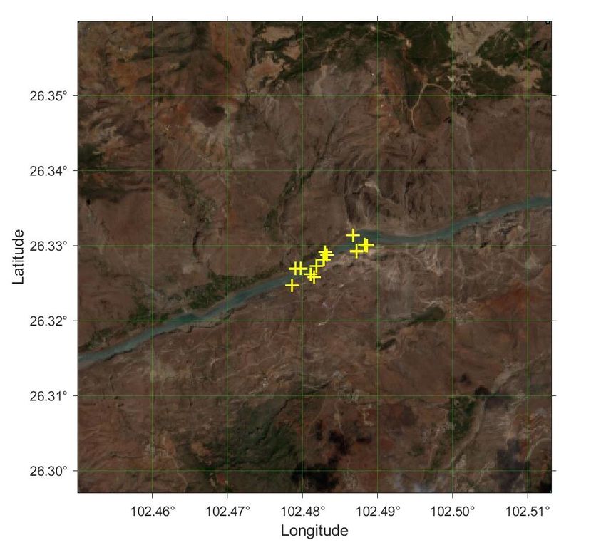
Figure 3.12: Time series of virtual station 8 ........................................................... 29
Figure 3.13: Time series of virtual station 9 ........................................................... 30
Figure 3.14: Time series of virtual station 10 ......................................................... 30
Figure 3.15: Time series of virtual station 11 ......................................................... 30
Figure 3.16: Time series of virtual station 12 ......................................................... 31
Figure 3.17: Time series of virtual station 13 ......................................................... 31
Figure 3.18: Time series of virtual station 14 ......................................................... 31
Figure 3.19: Time series of virtual station 15 ......................................................... 32
Figure 3.20: Comparison of waveforms which successful retracked by three meth
 ods, the first figure shows a specular waveform and the second figur
 e shows a flat patch waveform, the third and last figures show Brow
 n waveforms ........................................................................................... 32
Figure 3.21: Comparison of waveforms which successful retracked by two metho
 ds, the first two figures show specular waveforms and the last two fi
 gures show complex waveforms ........................................................... 33
Figure 3.22: Comparison of waveforms that successful retracking by one method.
 The top figure presents a flat patch waveform can be retracked by O
 cean retracker, the bottom figure presents a specular waveform can b
 e retracked by OCOG retracker ............................................................ 34
Figure 4.1: Waveform obtained from Virtual Station 11, cycle 5. The thermal noi
 se (background noise) segment doesn’t appear at the beginning of the
 waveform. ............................................................................................... 36
Figure 4.2: An example of peak property extraction .............................................. 37
Figure 4.3: Peak value would be removed when we applied a smooth filter on a
 high peakiness waveform ...................................................................... 38
Figure 4.4: Footprints of virtual station 1 cycle 11 ................................................ 39
Figure 4.5: An example of water extraction by using MNDWI ............................ 41
Figure 4.6: Line shapefile of the target river .......................................................... 42
Figure 4.7: An example of vegetation extraction based on adjusted footprints ... 44
Figure 5.1: Scatter plots of the waveform and environmental indicators for the ge
 neral result .............................................................................................. 47
Figure 5.2: Spearman rank correlation of the waveform and environmental indicat
 ors for the general result ....................................................................... 48
Figure 5.3: Scatter plots of the waveform and environmental indicators for the co
 mplex waveform..................................................................................... 51
Figure 5.4: Spearman rank correlation of the waveform and environmental indicat
 ors for the complex waveform ............................................................. 52
Figure 5.5: Scatter plots of the waveform and environmental indicators for the no
 rmal environment condition .................................................................. 55
 X

Figure 5.6: Spearman rank correlation of the waveform and environmental indicat
 ors for the normal environment condition ........................................... 55
Figure 5.7: Scatter plots of the waveform and environmental indicators for the co
 mplex environment condition ................................................................ 58
Figure 5.8: Spearman rank correlation of the waveform and environmental indicat
 ors for the complex environment condition ......................................... 58
Figure 5.9: Combined results of Indicators and water surface height in station 1
 ................................................................................................................ 60
Figure 5.10: Combined results of Indicators and water surface height in station 2
 ................................................................................................................ 60
Figure 5.11: Combined results of Indicators and water surface height in station 3
 ................................................................................................................ 61
Figure 5.12: Combined results of Indicators and water surface height in station 4
 ................................................................................................................ 61
Figure 5.13: Combined results of Indicators and water surface height in station 5
 ................................................................................................................ 62
Figure 5.14: Combined results of Indicators and water surface height in station 6
 ................................................................................................................ 62
Figure 5.15: Combined results of Indicators and water surface height in station 8
 ................................................................................................................ 63
Figure 5.16: Combined results of Indicators and water surface height in station 9
 ................................................................................................................ 63
Figure 5.17: Combined results of Indicators and water surface height in station
 10 ............................................................................................................ 64
Figure 5.18: Combined results of Indicators and water surface height in station
 11 ............................................................................................................ 64
Figure 5.19: Combined results of Indicators and water surface height in station
 12 ............................................................................................................ 65
Figure 5.20: Combined results of Indicators and water surface height in station
 13 ............................................................................................................ 65
Figure 5.21: Combined results of Indicators and water surface height in station
 14 ............................................................................................................ 66
Figure 5.22: Combined results of Indicators and water surface height in station
 15 ............................................................................................................ 66
Figure 5.23: The condition of proper tracking and anomaly tracking ........................ 67

 XI

XII

List of Tables

Table 1.1: Information about some altimetry mission since 1985 ............................ 2
Table 1.2: Conventional altimeter effective footprint diameters as a function of si
 gnificant wave height (Chelton et al., 1989) .......................................... 7
Table 2.1: Spectral bands for the MSI sensors (Sentinel-2) ................................... 11
Table 2.2: Spectral bands for the OLI and TIRS sensors (Landsat-8)................... 13
Table 2.3: Description of virtual stations.................................................................. 18
Table 3.1: Range and Geophysical corrections for the Sentinel-3B Level-2 product
 ................................................................................................................... 26
Table 5.1: Summary of indicator distribution for three groups .............................. 67
Table 5.2: Summary of indicator distribution refer to the height difference ......... 68

 XIII

XIV

1.1 Background of Satellite Radar Altimeter

Chapter 1

Introduction

Water covers more than seventy percent area of the earth's surface and the total volume
of water is approximately 333 million km3, including 97.47% saltwater and 2.53%
freshwater. Nevertheless, liquid freshwater that can be directly consumed by human
only account for 0.26% of the freshwater (Gleick, 1993). Global warming, caused by
the surge of greenhouse gas emissions leads to changes in the distribution of water re-
sources over many regions (S. Hagemann, 2013). Meanwhile, excessive consumption
of freshwater results in the drain of the ground and surface inland water (lakes, rivers,
etc.). The water crisis has aroused people's concern all over the world. Therefore, con-
tinuous monitoring of water bodies has been a critical task for human being in the past
decades and will continues to be one in the future.

There are two commonly used approaches for water body monitoring: 1) Gauging sta-
tion measurement, a traditional method to monitor water resources which can achieve
high accuracy but restricted by its distribution and high construction cost; 2) Satellite
altimetry, which has larger coverage and higher temporal resolution and continuous
measurements. The quality and accuracy of altimetry are not comparable with that of
the in-situ data because of errors from different sources. With the development of al-
timetry, especially the application of Delay-Doppler (SAR) altimeter, the aforemen-
tioned problems have been generally overcome in ocean application. However, low ac-
curacy and unreliable quality of data which are driven by altimeter performance and
post-processing technique over inland water bodies are still unfixed issues (Berry et al.,
2005).

To ensure the quality of data over inland water, the Open-Loop Tracking Command
(OLTC) is utilized on newly designed satellites (Jason-3, Sentinel-3). It is capable to
set a proper reception window of altimeter and to ensure that received waveform com-
ing from desired water bodies, supported by on-board pseudo-DEM tables and DORIS
system (Le Gac, 2019). The received waveform is exploited to extract geophysical pa-
rameters (water level, backscatter), but it is normally contaminated by the environment
within corresponding footprints (Tourian, 2012). This contamination changes the shape
of the waveform and complicates the construction of it, further results in failing to de-
termine the water level height. Therefore, it is important to understand the connection
between the environment and the waveform for the sake of further improvement of
measurement accuracy over inland water. In this thesis, we investigate the effect of the
environment within footprints on the waveform and its height products using the Syn-
thetic Aperture Radar (SAR) altimetry data obtained in OLTC mode, optical images,
and DEM data.
 1

1.1 Background of Satellite Radar Altimeter

1.1 Background of Satellite Radar Altimeter

American geophysicist W. M. Kuala officially formalized the concept of satellite altim-
etry at a Solid-Earth and ocean physics symposium in August 1968 and he emphasized
the importance of altimetry in geodesy and hydrology field (Kuala, 1968). Participants
made a proposal that develops an altimeter which has 10 cm level accuracy and 1° spa-
tial resolution in ten years. Over the years, altimetry technique has made a great contri-
bution to many fields. Figure 1.1 shows launched and planned altimetry missions since
1985. Table 1.1 presents information about launched and planned altimetry missions
since 1985.

 Figure 1.1: Operating period of altimetry satellite since 1985 (Open Altimeter database, TUM)

 Table 1.1: Information about some altimetry mission since 1985

 Satellite Agency Year H Altimeter f T I ε

 Range: 1m
 Skylab NASA 1973 435 S193 - - 50
 Orbit: about 5m
 Range: 5cm
 Seasat NASA 1978 800 ALT 13.5 17 108
 Orbit: about 1m
 Range: 4cm
 Geosat US Navy 1985 800 RA- 13.5 17 108
 Orbit: 30-50cm
 Range: 3cm
 ERS-1 ESA 1991 785 RA 13.8 35 98.5
 Orbit: 8-15cm
 Topex NASA Topex Range: 2cm
 1992 1336 13.6/5.3 10 66
 /Poseidon CNES Poseidon-1 Orbit: 2-3cm
 Range: 3cm
 ERS-2 ESA 1995 785 RA 13.8 35 98.5
 Orbit: 7-8cm

 2

1.1 Background of Satellite Radar Altimeter

 US Navy Range: 3.5cm
 GFO 1998 800 GFO-RA 13.5 17 108
 NOAA Orbit: /
 CNES Range: 2cm
 Jason-1 2001 1336 Poseidon-2 13.6/5.3 10 66
 NASA Orbit: 2-3cm
 Range: 2-3cm
 Envisat ESA 2002 800 RA-2 13.6/3.2 35 98.5
 Orbit: 2-3cm
 CNES
 NASA Range: 2.5cm
 Jason-2 2008 1336 Poseidon-3 13.6/5.3 10 66
 Eumestat Orbit:

1.2 Basics of altimetry waveform

demonstrated the concept of using the satellite altimeter for geoid determination. Alt-
hough noise level and systematic error were up to 1-3m and 10m, successful launch still
signified a big approach to the practical application (Leitao et al., 1976). Seasat,
launched in June 1978, was the first altimetry satellite applied in the oceanology field.
Its on-board altimeter first implemented dechirp pulse compression technology, which
significantly improved the resolution of altimeter (Tapley et al., 1982). Seven years later,
the USA Navy transmitted Geosat satellite which marks ocean geoid can be determined
from space (Cartwright et al., 1990). It was henceforth followed by a series of succes-
sively launched advanced altimetry satellites with different purposes: ERS, Topex/PO-
SEIDON, Jason1/2/3, Envisat, ICEsat1/2, Sentinel-3A/B

Although most of these satellites are initially designed for ocean applications, their con-
tinental application has been demonstrated since Rapley et al. (1987) firstly used Seasat
data to explore inland water targets. However, the aforementioned problems of the per-
formance of the altimeter and post-processing technique, restricted the reliability and
accuracy of data on inland water. Recently, benefitted from the Synthetic Aperture Ra-
dar (SAR) technique and the new OLTC tracking mode, the altimeter’s performance
over inland water has been significantly improved (Wingham et al., 2006; ESA, 2018;
Biancamaria, 2018). The remaining problem is the uncertainty of the returned echo
(waveform) during post-processing.

Variable conditions of different inland water and the complex environment within the
altimetry footprints (section 1.2.2) are the main factors that result in this uncertainty.
However, there have been very few researches dedicated to the relation between the
waveform and two aforementioned reasons. Berry et al. (2005) reported that different
sizes of water bodies present different shapes of the returned waveform, and classified
them into four groups accordingly. Remy et al. (2012) indicated that waveform is influ-
enced by snow characteristics fluctuation, and leads to the variation of the leading edge
width in the central part of East Antarctica. Maillard et al. (2015) took environmental
factors (river shape and width) into account to improve the precision of altimetry meas-
urements of the water level. These papers focused on determining a single environmen-
tal factor and solving a specific problem, rather than comprehensively considering mul-
tiple factors. As a matter of fact, the waveform is associated with various environmental
factors including the variation of elevation, coverage of the surface, the position of the
water body within the footprints and so on. How these factors impact the shape of the
waveform is still uncertain.

1.2 Basics of altimetry waveform

The basic content of altimetry is complicated and covers multiple fields. Therefore,
only two concepts that are closely related to this thesis are presented in this section.

1.2.1 Satellite altimetry waveform

The waveform in altimetry data is a temporal profile (Marth et al., 1993) describing
accumulated and smoothed power scattered from a ground object and received by the
 4

1.2 Basics of altimetry waveform

on-board altimeter. The process of interacting between emitted pulse and scattering sur-
face as well as its corresponding part in the waveform shown as follow schematic.

Figure 1.2: Interaction of pulse and scattering surface, and construction of waveform (Gao, 2020)

 1. 0< t < t0, altimeter emits radar pulses towards the earth surface in nadir direction.
 Pulses emitted by antenna form a semi-spherical shell. The width of this shell
 determined by pulse duration ∆ and width of pulse ∆ is altimeter’s range
 resolution.
 2. t = t0, pulse front faces and illuminates nadir points and a return echo begins to
 return toward altimeter.
 3. t0< t < t1, illuminated area continuously grows and forms a growing disc cen-
 tered on nadir point until trailing edge reaches the surface. During this period,
 altimeter receives powers from antenna beam-limited area. Ascent part of wave-
 form corresponds to this period
 4. t = t1, illuminated area stops increasing and begins to form an annular ring at the
 same time keeping area constant. This epoch corresponds to the peak point of
 waveform, received power to reach its maximum.
 5. t1< t < t2, the illuminated ring is getting larger and narrower, but still keep area
 constant. In this period, received power reflected from outside of antenna beam-
 limited area. It results in the declination of power and forms the trailing part of
 the waveform.

In general, a received signal undergoes different Rayleigh fluctuations when altimeter
moves along the orbit and path lengths to multiple facets change (Chelton et al., 1989).
Many individual waveforms must be averaged to obtain a mean and smooth waveform.

 5

1.2 Basics of altimetry waveform

The averaged waveform (Figure 1.2 bottom) is mean returned power series which rec-
orded by altimeter (Brown, 1977), it consists mainly of three parts:

 1. The thermal noise: This noise is generated by altimeter before it receives the
 first return signal. It remains a constant power level to return waveform.
 2. The leading edge: It is the main part of the waveform where maximum power
 return from ground occurs on. The Surface Wave Height (SWH) and range be-
 tween satellite and scattering surface at nadir point (if surface is ocean) can be
 extracted from this part.
 3. The Trailing edge: Decaying return power in this part result in the trailing edge.
 It can be approximated by a straight line whose slope depends on the altimeter
 antenna pattern and the off-nadir angle (Chelton et al., 2001).

Mean sea level corresponds to half of the distance between wave crests and troughs. It
can be determined by tracking the half power point on the leading edge. SWH can be
determined from the slope of the leading edge of the returned waveform in the vicinity
of the half-power point (Chelton et al., 1989).

The waveform characteristics mentioned above are appropriate for waveform extracted
from ocean and large lakes, but not for inland water application. Berry et al. (2005)
classified waveform from different lakes to four types as shown in Figure 1.3. Decreas-
ing the size of the lake, the number of Brown model waveforms decreases, and quasi
specular waveforms occur more times. Occurrence frequency of flat patch waveforms
is highest among four types for the case of a s mall water body.

 Figure 1.3: Example of four different types of waveform
 6

1.2 Basics of altimetry waveform

The situation on rivers is more complex than lakes because the shape of a river is nor-
mally a narrow square or even a line, making it more difficult for altimeter to acquire
water information from rivers. Meanwhile, the environment surrounds the river affects
more on the shape of the waveform, the position of the leading edge and power ampli-
tude.

1.2.2 Footprints

The footprint of a conventional radar altimeter is the area on water surface illuminated
by the antenna beam angle defined by the half power point of the antenna gain (Chelton
et al., 1989). In principle, the effective footprint area can be calculated from the pulse
duration , altitude of the satellite 0 , the radius of earth and significant wave
height H1/3 which is approximate to the crest-to-trough height of the 1/3 largest waves
in the footprint. Taking two satellites whose altitudes are 800 km and 1335 km as an
example, the effective footprint diameters computed from equation 1.2.1 are presented
in Table 1.2.

 0 ( + 2 1 )
 3
 = 0 (1.2. 1)
 1+ 
 
Table 1.2: Conventional altimeter effective footprint diameters as a function of significant wave
 height(Chelton et al., 1989)
 Effective footprints diam- Effective footprints diam-
 H1/3 (m) eter (R0 = 800km) eter (R0 = 1335km)
 (km) (km)
 0 1.6 2.0
 1 2.9 3.6
 3 4.4 5.5
 5 5.6 6.9
 10 7.7 9.6
 15 9.4 11.7
 20 10.8 13.4

The Delay Doppler/SAR altimeter (SAR mode) is different from the conventional radar
altimeter as it implements coherent processing of groups of transmitted pulses. Its pro-
cessor allows to sharpen the area of the pulse in the along-track direction. The Doppler
beam formation in SAR mode allows to discriminate the direction of arrival of the ech-
oes in the along-track direction instead of the measure of the time delay. Hence, the
width of footprints is defined independently in both independent directions, the along-
track and the across-track directions. In the across-track direction, the width of foot-
prints is defined as the radius of conventional altimeter footprints. However, in the
along-track direction, the width of the footprint is defined as the sharpened beam-lim-
ited area which can be calculated by equation 1.2.2 (ESA, 2018)
 7

1.2 Basics of altimetry waveform

 =ℎ (1.2. 2)
 2 64

 Figure 1.4: Comparison of conventional (a) and SAR (b) altimetry’s footprints (Gao, 2020)

Figure 1.4a is schematic of altimeter measuring in conventional mode (LRM). Center
region presents ideal footprints, each annulus indicates different time delay and returns
different delay pulse. Figure 1.4b is schematic of altimeter measuring in SAR mode
whose along-track resolution has been significantly improved and across-track resolu-
tion remains the same, its footprints is the swath in the center.

 8

2.1 Data

Chapter 2

Data and case study

As mentioned in chapter one, this thesis is dedicated to assessing the relation between
altimetry waveform, water level, and the environment within its corresponding foot-
prints. Waveform and water level can be obtained from altimetry data. The environmen-
tal conditions can be evaluated by remote sensing images and DEM data. Therefore, in
this chapter, we firstly introduce Sentinel-3 altimetry data, Sentinel-2 and Landsat-8
image data, and STRM DEM data which are used for our purpose. Afterward, the case
study is presented in the second section. For the sake of diversity of the environmental
conditions, we selected two types of rivers: rivers in the valley and rivers in the plain
area. In addition, these rivers have different water flow and climate conditions. At the
end of the chapter, we would determine fourteen virtual stations located on two rivers
with the help of remote sensing images.

2.1 Data

2.1.1 Sentinel-3 data

Sentinel-3 satellites are jointly designed and operated by ESA and EUMETSAT as part
of the European Commission Copernicus program, which aims to monitor earth for
global environment and security. It can provide multiple sorts of data about sea surface
topography, sea and land surface temperature, and ocean and land surface color with
high accuracy and reliability. The Sentinel-3 mission is based on two identical satellites
flying on a polar, Sun-synchronous orbit at altitude 815 km, an inclination of 98.6°, a
repeat cycle of 27 days and having a 140 degrees orbit phase difference between twins.
First satellite, Sentinel-3A, was launched on 16 February 2016. Sentinel-3B which dou-
bled the coverage of mission became the second member of the constellation on 25
April 2018.

Embarked instruments on Sentinel-3 are shown as follow:

 - A push-broom imaging spectrometer instrument called the Ocean and Land
 Color Instrument (OLCI). A dual view (near-nadir and backward views) conical
 imaging radiometer called the Sea and Land Surface Temperature Radiometer
 (SLSTR) instrument. OLCI and SLSTR are devoted to optical imagery acquisi-
 tion.
 - A dual-frequency SAR altimeter called the SAR Radar Altimeter (SRAL) oper-
 ating in Ku band (15.575 GHz) and C band (5.42 GHz). SRAL can operate in
 SAR (Synthetic Aperture Radar) or LRM (Low Resolution Mode) processing
 9

2.1 Data

 mode.
 - A Microwave Radiometer (MWR) instrument and OLTC Tracking mode (more
 detail on section 3.1.1 supporting the SRAL by providing wet atmosphere cor-
 rection and maintaining a stable tracking control.
 - A Precise Orbit Determination package including a Global Navigation Satellite
 Systems (GNSS) instrument, a Doppler Orbit determination and Radio-posi-
 tioning Integrated on Satellite (DORIS) instrument and a Laser Retro-Reflector
 (LRR). These systems are used to precisely calculate the satellite orbit.

Two follow-on satellites Sentinel-3C and Sentinel-3D are planned to launch in 2021.

 Figure 2.1: Sentinel-3 and payload instrument (Credit: ESA)

For our water level application, Level 2 product produced by SRAL altimeter has been
used. SRAL is a redundant dual-frequency (C-band and Ku-band) instrument for deter-
mining the two-way delay of the radar echo from the Earth's surface with a precision
better than a nanosecond (ESA, 2018). It has two observation modes: Low Resolution
Mode (LRM) and Synthetic Aperture Radar (SAR) mode.

LRM mode is the conventional altimeter pulse limited mode in which Pulse Repetition
Frequency (PRF) is about 1924Hz. These pulses are transmitted toward the ground fol-
low a model of 3 Ku band pulses + 1 C band pulse + 3Ku band pulses. On-board altim-
eter processes and average pulses to produce a 128 bins waveform every 50.9 ms.

SAR mode is the high along-track resolution mode based on Synthetic Aperture Radar
technique. The PRF is about 17800 Hz in SAR mode. Transmitted pulses consist of Ku-
band bursts and two C band pulses at the two sides of each burst. Each burst contains
66 pulses (1 C band pulse + 64 Ku band pulses + 1 C band pulse), corresponding to a
duration of 12.74 ms.
 10

2.1 Data

Sentinel-3 has three levels of products in which level 0 product is original measure-
ments and it isn’t provided to common users, level 1 (B) product is processed by several
steps (i.e. calibration, beam pointing, beam steering, beam stacking, muti-look, etc),
and level 2 product that we used in this thesis. The Level 2 products are divided into
Land (SR_2_LAN__) and Marine (SR_2_WAT__) products over different areas. Marine
Products contain information sensed over the open ocean, the coastal areas, the sea-ice
and over part of the land within a certain distance from the coastline. As far as Land
Products contain information sensed over land, the coastal areas, land ice and inland
water (ESA, 2018).

2.1.2 Sentinel-2 data

The Copernicus Sentinel-2 mission contains a constellation that consists of two polar-
orbiting satellites operated in a 786 km high sun-synchronous orbit, with an inclination
of 98.62° and a 180° phase difference between twins. The first satellite Sentinel-2A was
launched on 23 June 2015, and its twins Sentinel-2B was transmitted on 7 March 2017.
The mission aims at monitoring variability in land surface conditions, and its swath is
290 km width and 10 days revisit cycle for each satellite (5 days with 2 satellites at the
equator) will support monitoring of Earth's surface changes. The limitation of satellite
coverage is from between latitudes 56° south and 84° north.

 Figure 2.2: Sentinel-2 satellite (Credits: ESA)

Each of the Sentinel-2 satellites carries a single multi-spectral instrument (MSI) with
13 spectral channels in the visible/near-infrared (VNIR) and short wave infrared spec-
tral range (SWIR). MSI uses a push-broom concept whose sensor works by collecting
rows of image data in the direction across satellite track and producing new rows for
acquisition with the forward motion of satellite along the orbit. The average period of
observation over land and coastal areas is approximately 17 minutes and the maximum
period of observation is 32 minutes.

 11

2.1 Data

 Table 2.1: Spectral bands for the MSI sensors (Sentinel-2)

 S2A S2B

 Central Central Spatial
 Bandwidth Bandwidth
 Band Number wavelength wavelength resolution
 (nm) (nm)
 (nm) (nm) (m)
 Band 1 - Coastal aerosol 442.7 21 442.3 21 60
 Band 2 - Blue 492.4 66 492.1 66 10
 Band 3 - Green 559.8 36 559.0 36 10
 Band 4 - Red 664.6 31 665.0 31 10
 Band 5 - Vegetation red edge 704.1 15 703.8 16 20
 Band 6 - Vegetation red edge 740.5 15 739.1 15 20
 Band 7 - Vegetation red edge 782.8 20 779.7 20 20
 Band 8 - NIR 832.8 106 833.0 106 10
 Band 8a - Narrow NIR 864.7 21 864.0 22 20
 Band 9 - Water Vapour 945.1 20 943.2 21 60
 Band 10 - SWIR - Cirrus 1373.5 31 1376.9 30 60
 Band 11 - SWIR 1613.7 91 1610.4 94 20
 Band 12 - SWIR 2202.4 175 2185.7 185 20

Similar to Sentinel-3, Sentinel-2’s products have three levels that provide different
kinds of images with different processing methods. In our research, we used Level-2
products which have finished the atmospheric correction and radiometric calibration.
That means we can directly execute classification and extract environmental properties
from them.

2.1.3 Landsat-8 data

Landsat-8 is the eighth satellite in the Landsat program, which is collaboratively oper-
ated by National Aeronautics and Space Administration (NASA) and the United States
Geological Survey (USGS). It was launched on 11 February 2013, flying in a sun-syn-
chronous, near-polar orbit, at an altitude of 705 km, inclined at 98.2°, an orbital period
of 99 minutes, and a 16-day repeat cycle. Landsat-8 can collect and archive medium
resolution (30-meter spatial resolution) multispectral image data affording seasonal
coverage of the global landmasses for more than 5 years. It carries a two-sensor payload
comprise of the Operational Land Imager (OLI), built by BATC, and the Thermal In-
frared Sensor (TIRS), built by NASA GSFC. Both the OLI and TIRS sensors simulta-
neously image every scene but can be independently exploited if a problem in either
sensor arises (USUG, 2019). The OLI sensor collects image data for 9 shortwave spec-
tral bands over a 190 km swath with a 30 m spatial resolution for all bands except the
15 m Pan band, and the TIRS sensor collects image data for two thermal bands with a
100 m spatial resolution over a 190 km swath (Table 2.2).

 12

2.1 Data

 Figure 2.3: Illustration of the Landsat 8 Satellite (Credits: USUG)

 Table 2.2: Spectral bands for the OLI and TIRS sensors (Landsat-8)

 Band Number wavelength (μm) Spatial resolution(m)

 Band 1 - Coastal aerosol 0.435 - 0.451 30
 Band 2 - Blue 0.452 - 0.512 30
 Band 3 - Green 0.533 - 0.590 30
 Band 4 - Red 0.636 - 0.673 30
 Band 5 - NIR 0.851 - 0.879 30
 Band 6 - SWIR-1 1.566 - 1.651 30
 Band 10 - TIR-1 10.60 - 11.19 100
 Band 11 - TIR-2 11.50 - 12.51 100
 Band 7 - SWIR-2 2.107 - 2.294 30
 Band 8 - Pan 0.503 - 0.676 15
 Band 9 - Cirrus 1.363 - 1.384 30

In this thesis, we used the Level 1C Landsat-8 product which is also post-processed by
geometric and radiometric correction. Environmental properties can be directly ex-
tracted from the product without further processing. The spatial resolution of images
for Landsat-8 (30 m) is lower than Sentinel-2 (20m). Therefore, Landsat-8 is the sup-
plementary data in the case of river targets are covered by cloud or shadow in Sentinel-
2 images.

2.1.4 Shuttle Radar Topography Mission data

The Shuttle Radar Topography Mission (STRM) is an international project spearheaded
by the U.S. National Geospatial-Intelligence Agency (NGA) and the U.S. National Aer-
onautics and Space Administration (NASA). It aims at obtaining digital elevation mod-
els on a near-global scale from 56°S to 60°N, generating the most complete high-reso-
lution digital topographic database of Earth prior to the release of the ASTER GDEM
in 2009. DEM data was acquired through a specially modified radar system that flew
 13

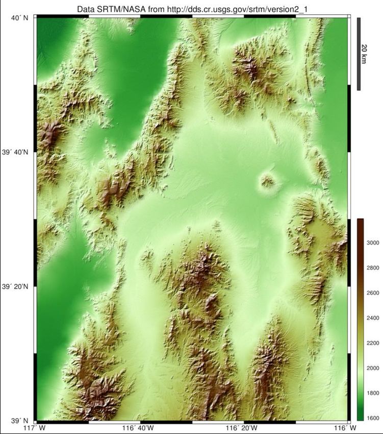
2.2 Case study

on-board the Space Shuttle Endeavour during the 11-day STS-99 mission in February
2000.

 Figure 2.4: Example of a map of Nevada from SRTM1 data (Credits: USGS)

The resolution of the original data is one arcsecond (30 m). The coverage includes Af-
rica, Europe, North America, South America, Asia, and Australia. However, the data is
only available to governments. Hence, the product we used in this thesis is STRM 3
and its resolution is three arcseconds (about 90 m). Considering the size of SAR foot-
prints is about 330 m·2000 m (general condition), STRM 3 is sufficient for describing
the topography within the footprints.

2.2 Case study

2.2.1 Yarlung Tsangpo River
 14

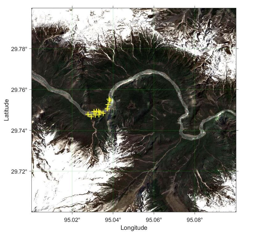
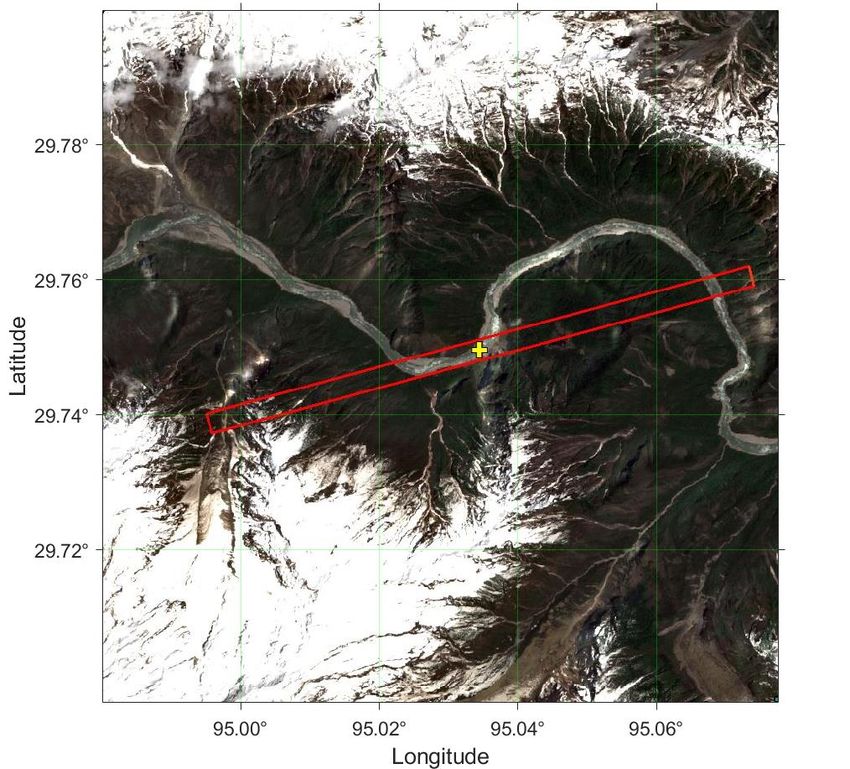
2.2 Case study

The Yarlung Tsangpo River is the longest plateau river in China, located in Tibet Au-
tonomous Region. It is one of the highest rivers in the world. The river originated from
the Jemajangzong Glacier, the north of the Himalaya mountains in southwest Tibet,
whose upstream also called Maquan River. The Yarlung Tsangpo River flows across the
south of Tibet from west to east and turns southward at the easternmost peak of Hima-
laya. It flows out of Chinese territory through Bhashika in the end. The river is 2900
km long with a basin area of 6.17·105 km. 2057 km of the total length and 2.4·105 km2
of the basin areas are located within China. The mainstream above Lazi is upstream.
The lowest point of the riverbed of the upstream is at 3950 m above sea level, which is
the alpine valley zone.

The annual variation of precipitation in the Yarlung Tsangpo River basin is small and
its distribution is uneven. The wet season is from July to September, accounting for 50%
to 80% of the annual precipitation. Meanwhile, more meltwater from snow and ice
flows into the rivers during the months with the most rainfall, as resulting in a high
water level. The annual precipitation of the YarlungZangbo River is less than 300 mm
in upstream and higher than 300 mm in midstream which belongs to the plateau tem-
perate climate. However the downstream of the basin is high temperature and rainy,
with an average annual rainfall of more than 4000 mm near Basica. Most of the virtual
stations (Figure 2.5) of Yarlung Tsangpo River are located in the upstream and mid-
stream of the river.

 Figure 2.5: Part of the Yarlung Tsangpo River and the location of virtual station 1 (yellow cross)
 15

2.2 Case study

2.2.2 Yangtze River

The Yangtze River originates from the Ratandon peaks in the Qinghai-Tibetan Plateau,
flows through 11 provincial administrative regions include Qinghai, Tibet, Sichuan and
Shanghai more than 6300 km. It runs through an area of about 2·106 km2 before finally
discharging into the East China Sea in the east of Chongming Island. It is the largest
river in Asia in terms of water discharge and the third-longest river in the world (Milli-
man et al., 1983).

The upstream of the Yangtze River (serval virtual stations located in this reach), also
known as Jinsha River (Figure 2.6), has a basin area of 5·105km2, accounting for about
26 percent of the Yangtze River basin area. The middle and upper reaches of the Jinsha
River are surrounded by valleys except for the estuary of tributaries, where the river
valley is slightly wider, the slope of most valleys is between 35° and 45° and more than
60° ~ 70° for some cliffs. It is worth mentioning that water height difference of the river
is large. The difference can reach 220m in ten kilometers.

 Figure 2.6: Part of the Jinsha River and the location of virtual station 8 (yellow cross)

People usually call the Yangtze River as Chang River in China. Yangtze is the old name
for the downstream of the Chang River, covering the area from Nanjing to its estuary.
Different from the upper reaches, the lower reaches are flat with an average elevation
 16

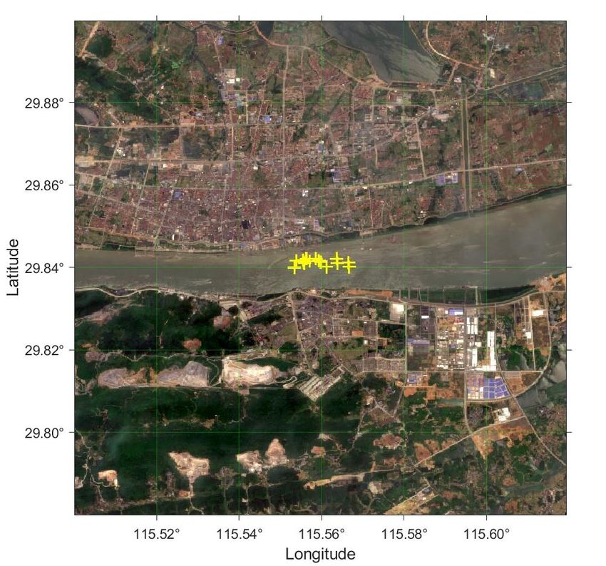
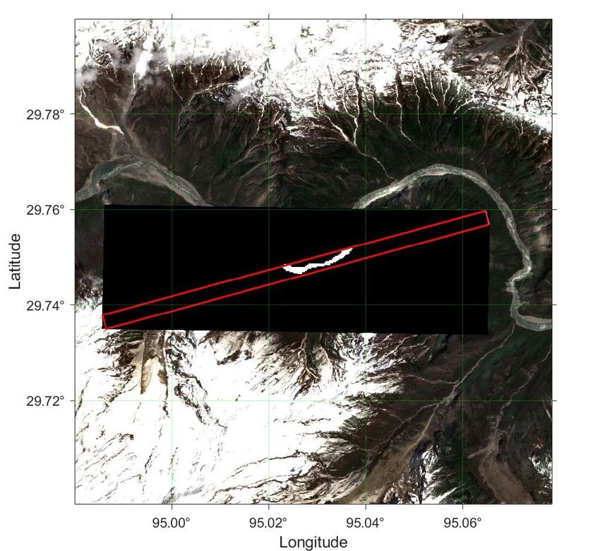
2.3 Virtual station

of less than 500 meters. Beginning from Nanjing city, the river gradually gets wider
(Figure 2.7) and develops towards the estuary in the shape of a trumpet. By the time it
reaches the estuary, the river can achieve 80 kilometers wide.

 Figure 2.7: Part of the Yangtze River and the location of virtual station 15 (yellow cross)

2.3 Virtual station

A virtual station can be determined on an intersection point of the target river and the
ground track of Sentinel-3 with a given search radius (5 km). Each time the satellite
passes over the river, ground tracks have a slight drift to the set virtual station. As shown
in Figure 2.8, the yellow cross is the position of virtual station 8, blue lines indicate the
drifted ground tracks. Different from the ocean application, in order to get more accu-
rate range measurements and avoid hooking effect over inland water, water and land
surfaces surrounding the virtual station are supposed to be distinguished by remote
sensing images. Furthermore, the resolution of the along-track direction is about 330
meters while the width of rivers is in the same or a smaller magnitude, which means
only one or two samples in each cycle can obtain the proper waveform from the river.
Not only distinguishing the type of surfaces is important, but also, we should select the
one sample data which is located nearest to the virtual station or the river.

 17

2.3 Virtual station

 Figure 2.8: Schematic of Virtual Station 8

The description of the virtual station is present in Table 2.3. The chosen station evenly
distributed on two kinds of topography and the elevation surround it should be docu-
mented in on-board DEM table. Station 7 is located on a small tributary of the Yangtze
River, and not recorded in the OLTC database. Therefore, the virtual station 7 didn’t
involve subsequent processing.

 Table 2.3: Description of virtual stations

 No. Latitude Longitude Direction Track River

 1 29.7454 95.0321 Ascending 53 Yarlung Tsangpo River
 2 29.7475 95.1206 Descending 161 Yarlung Tsangpo River
 3 29.9016 95.1615 Descending 161 Yarlung Tsangpo River
 4 29.0439 93.3518 Ascending 324 Yarlung Tsangpo River
 5 29.0397 93.0589 Descending 47 Yarlung Tsangpo River
 6 29.2564 92.1823 Descending 375 Yarlung Tsangpo River
 7 29.7493 95.9660 Ascending 110 Yangtze River

 18

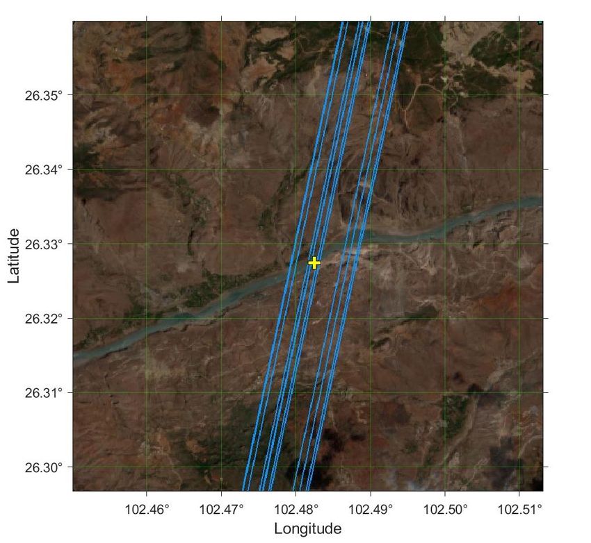
2.3 Virtual station

8 26.3227 102.4822 Ascending 67 Jinsha River
9 26.3344 102.6306 Descending 289 Jinsha River
10 27.4171 103.1350 Ascending 124 Jinsha River
11 28.9072 108.3504 Ascending 82 Yangtze River
12 26.6480 106.1244 Ascending 296 Yangtze River
13 25.7780 109.0320 Descending 303 Yangtze River
14 25.7328 109.1833 Ascending 82 Yangtze River
15 29.8363 115.5811 Ascending 153 Yangtze River

 19

3.1 Measuring principle

Chapter 3

Water level generation from altimetry data

Altimetry waveform can be directly obtained from satellite data, while the water level
must be calculated by the altitude of the satellite, range measurements between the sat-
ellite and target water, and several corrections. The technique exploited to accurately
acquire the range is referred to as waveform retracking. The results from three retrack-
ing methods: SAMOSA-3 retracker, Ice-sheet retracker and OCOG retracker, are used
in this thesis. After accurate range measurement is determined, several geophysical and
range corrections also should be applied to eliminate propagation errors and geophysi-
cal errors. In this chapter, we investigate the waveform and water levels of our target
water bodies. More specifically, we introduce the principle of water level generation
from satellite altimetry data and demonstrate its result of fourteen virtual stations.

3.1 Measuring principle

 Figure 3.1: the principle of satellite altimetry measurement (Nielsen et al., 2017)

On-board radar altimeter transmits high-frequency signals toward Earth and receives
the power returned from the surface. They referred to a time dependence measurement
to make the round trip between the satellite and the surface. If this precise measurement

 20

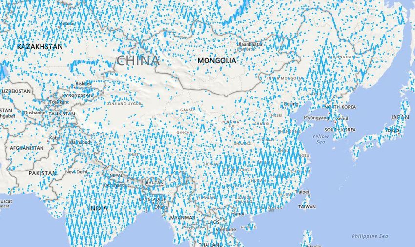
3.1 Measuring principle

of round trip is recorded, the range measurements , the one-way distance, can be de-
termined. The Sea Surface Height ( ) is the height of the sea surface with respect to
a reference ellipsoid. Figure 3.1 is the schematic of the satellite altimetry measurement
principle and physical significance for each parameter.

3.1.1 Tracking system

As shown in Figure 3.1, the position of range window (reception window) decides
whether the altimeter properly receives the pulse from water. The position is set by the
tracking system which is normally referred as a tracker. In other words, the tracker
guarantees the quality of range measurements by controlling when and how altimeter
acquiring return signal. It has two different tracking modes: the “Closed-Loop” mode
(CL) and the “Open-Loop” mode (OL). CL, also called autonomous mode, requires the
acquisition phase to set up altimeter’s reception window. OL, also called Diode/DEM
on altimeters, allows signal tracked inside reception window, contributes to prior pa-
rameters in on-board pseudo-DEM tables (Le Gac et al., 2019). OLTC is a new tracking
technique applied for open-loop mode on Sentinel-3. It is capable of roughly evaluating
the relative position between satellite and water targets, and accordingly setting the
proper reception window based on elevation information recorded in on-board tables
and navigation bulletin provided by DORIS system.

 Figure 3.2: Hydrology Targets database defined for Sentinel-3B in China and its surrounding area
 (Credits: ESA)

ESA and its collaboration agency established an online database to collect hydrology
targets data for OLTC application on Sentinel-3 mission (https://www.altimetry-hy
dro.eu/). Users from all over the world can contribute to this database. Sentinel-3A’s
latest upgrade on its OLTC on-board table was on March 9, 2019. Sentinel-3B upgraded
its on-board table on November 27, 2018. There are more than thirty thousand hydrol-
ogy targets recorded in Sentinel-3 on-board table which supports the altimeter acquiring
high quality data.

 21

3.2 Improving range using waveform retracking

Le Gac et al. (2019) compared the performance of open-loop and closed-loop by Sen-
tinel-3B measurements. The result indicated that the success rate of retracking is sig-
nificantly higher, especially for small lakes (from 67% to 84%) and rivers (63% to
83%). The small lakes and rivers are also the focus in this thesis. To improve the quality
of data, we only exploited the measurement acquired in open-loop mode.

3.1.2 Water level calculation

The sea surface height can be calculated by (Dinardo, 2020):

 1 1
 = − ( ∙ ∙ 0 + ∙ _ + ) (3.1. 1)
 2 2
Where:

 - is the sea surface height
 - is the altitude of the satellite center of mass above the reference ellipsoid,
 it can be precisely acquired with the help of Doppler Orbitography and Ra-
 dioposition Integrated by Satellite (DORIS) and Global Positioning System
 (GPS)
 - is the speed of light in vacuum
 - _ is the two-way tracker time delay between the pulse trans-
 mission and reference tracking point, corrected by all the instrumental effects.
 It can be accurately acquired with the help of the tracking system
 - is the range and geophysical correction over the sea. It will be intro-
 duced with more details in section 3.3

The inland water surface height (WSH) can be derived by:

 1 1
 = − ( ∙ ∙ 0 + ∙ + ) (3.1. 2)
 2 2
Where is the range and geophysical correction over land. It will be elaborated
in section 3.3 as well.

3.2 Improving range using waveform retracking

All altimeter data over different surfaces must be post-processed to generate accurate
range measurements between satellite and water targets. This post-processing so-called
waveform retracking is done by computing the departure of the waveform’s leading
edge from the altimeter tracking gate and offsetting the satellite range measurement
error accordingly (Figure 3.3). In essence, waveform retracking aims at finding the
mid-power point of leading edge and offsetting tracking gate to this point.

 22

3.2 Improving range using waveform retracking

 Figure 3.3: Schematic of waveform retracking (Tourian, 2012)

SRAL is a dual-frequency SAR altimeter, which we use for extracting inland water
surface height in this thesis. There are four waveform retracking algorithms (retracker)
for SRAL that are deputed to retrieve geophysical measurements for different types of
surface:

 - SAMOSA-3 retracker over open ocean and coastal zones
 - Ice-Sheet retracker (MLE4) over ice sheets
 - OCOG retracker over sea-ice margins
 - Sea-Ice retracker over sea ice

Shu et al. (2020) indicated that Sea-Ice retracker was unable to be applied on inland
water bodies, as the result of the high rate of missing data. Therefore, Sea-Ice retracker
would not be introduced in this thesis.

3.2.1 SAMOSA-3 retracker

SAMOSA model is a compact closed-form model for the SAR altimetry return wave-
form from the ocean, developed within the framework of an ESA-funded project on
the development of SAR Altimetry Mode Studies and Applications over the ocean,
coastal zones and inland water (SAMOSA).

SAMOSA-3 is an ocean retracking model in SAMOSA project which assumes Ocean
Gaussian statistics and is sensitive to surface roughness (Jain, 2014). Model’s parame-
ters are waveform epoch , significant wave height , Pu waveform amplitude
 , surface RMS slope, skewness and mis-pointing angle . The Doppler Frequency
 23