Interplay between intra-urban population density and mobility in determining the spread of epidemics.
←
→
Page content transcription
If your browser does not render page correctly, please read the page content below
Interplay between intra-urban population density and mobility in
                                                                              determining the spread of epidemics.

                                                                       Surendra Hazarie,1, ∗ David Soriano-Paños,2, ∗ Alex Arenas,3
                                                                            Jesús Gómez-Gardeñes,2, 4, † and Gourab Ghoshal1, 5, ‡

                                                                                     1
                                                                                         Department of Physics & Astronomy,
arXiv:2102.00671v1 [physics.soc-ph] 1 Feb 2021

                                                                            University of Rochester, Rochester, NY, 14627, USA.
                                                                  2
                                                                      GOTHAM Lab – Department of Condensed Matter Physics and
                                                               Institute for Biocomputation and Physics of Complex Systems (BIFI),
                                                                              University of Zaragoza, E-50009 Zaragoza, Spain.
                                                                        3
                                                                            Departament d’Enginyeria Informàtica i Matemàtiques,
                                                                         Universitat Rovira i Virgili, E-43007 Tarragona, Spain.
                                                                             4
                                                                                 Center for Computational Social Science (CCSS),
                                                                                    Kobe University, Kobe 657-8501, Japan.
                                                  5
                                                      Department of Computer Science, University of Rochester, Rochester, NY, 14627, USA.

                                                                                                     Abstract

                                                    In this work, we address the connection between population density centers in urban areas,
                                                 and the nature of human flows between such centers, in shaping the vulnerability to the onset of
                                                 contagious diseases. A study of 163 cities, chosen from four different continents reveals a universal
                                                 trend, whereby the risk induced by human mobility increases in those cities where mobility flows are
                                                 predominantly between high population density centers. We apply our formalism to the spread of
                                                 SARS-COV-2 in the United States, providing a plausible explanation for the observed heterogeneity
                                                 in the spreading process across cities. Armed with this insight, we propose realistic mitigation
                                                 strategies (less severe than lockdowns), based on modifying the mobility in cities. Our results
                                                 suggest that an optimal control strategy involves an asymmetric policy that restricts flows entering
                                                 the most vulnerable areas but allowing residents to continue their usual mobility patterns.

                                                 ∗
                                                      These two authors contributed equally to this work.
                                                 †
                                                      gardenes@unizar.es
                                                 ‡
                                                      gghoshal@pas.rochester.edu

                                                                                                        1
I. Introduction
During the last century, humankind has rapidly evolved into an interconnected society driven
by the existence of a vast mobility network connecting different areas around the globe. In
particular, the striking growth experienced by the international mobility network [1] has
helped to bridge socio-cultural [2–4] and economic gaps [5]. Accompanying this is the phe-
nomenon of urbanization, whereby a majority of the world’s population reside in densely
packed urban centers, with the trend only accelerating [6, 7], given the socioeconomic ad-
vantages that cities afford [8, 9]. Allayed against these benefits, the increase in mobility has
removed the main bottleneck limiting the spatial diffusion of confined epidemic outbreaks.
Once the disease spreads to different regions, it takes advantage of the high population
density and infrastructure networks in cities [10] to rapidly spread through the local popu-
lation. As a consequence, over the past few years, several contagious disease outbreaks have
emerged, notable among them H1N1 in 2009 [11], Ebola in 2014 [12], ZIKV in 2015 [13]
and of course more recently SARS-COV-2 [14, 15]. Indeed, the frequency with which these
pandemics occur is troublingly increasing [16].
Despite the different nature of the pathogens, their spreading, both globally and locally,
is primarily explained by the sequential combination of case importation from contagion
sources, followed by local community transmission converting initially unaffected regions
into new endemic areas. Different flavors of mobility play a role in each process: on the one
hand, long-haul flights [17] are usually the drivers facilitating the entry of pathogens into a
given country, to the extent that the airport mobility network has proved to be a reliable
proxy to determine pathogen arrival times [18], international infection routes [19], and to
complement phylogeographic inference of emerging pathogens such as SARS-CoV-2 [20]. On
the other hand, once index cases are found within a given region, a complex combination of
the local mobility [21] and socio-economic features of the population [22, 23] determines the
speed of epidemic spread and the extent of its outbreak.
Quantifying the impact of local mobility on the global diffusion of a pandemic constitutes
a challenging task. In this sense, several examples addressing the impact of daily recur-
2rent mobility patterns on the spread of contagious diseases can be found in the literature
[24–31]. The majority of these, however, are theoretical frameworks analyzing the features
of synthetic mobility networks, and the influence of total volume of travelers on the course
of the epidemic. Nonetheless, recent advances made in data-gathering techniques allow for
obtaining accurate representations of daily urban rhythms constructed from mobile phone
traces [32], geolocalized tweets [33], Location Based Social Networks [34], or extensive cen-
sus surveys. These data sets enable the extension of the theoretical machinery to address
real epidemic scenarios. Indeed, recurrent mobility patterns have been already useful for
identifying the most exposed areas in some epidemic scenarios [35] as well as reproducing
the infection routes of H1N1 influenza [36], Malaria [37], and more recently SARS-COV-2
[38–41].
While much attention has been spent on reconstructing past infections, or epidemic forecast-
ing in the case of extant pandemics, an important question that immediately arises, is what
makes regions—in particular urban agglomerations where most people reside—vulnerable to
the spread of pathogens in the first place? While factors such as population density, levels
of healthcare, quality of infrastructure and socioeconomic disparities play a major role [42],
vulnerability to spread is a complex interplay between these features that is, in general,
difficult to disentangle. For instance, the role of population density is an open question with
evidence both for and against its influence on epidemic spreading [43, 44]. Indeed, merely
the density of contacts, while relevant at a neighborhood level, is not enough to explain the
mechanisms of spread; one would also need to consider the mobility network of flows that
govern the exchange of people between the regions. In such a setting, the spatial distribu-
tion of the population densities and the strength of interaction between the regions become
especially relevant.
In other words it is reasonable to assume that the morphology of the city in terms of how
its residents are distributed and how they navigate the city plays a crucial role in their
susceptibility to pandemics. Indeed, recent studies have shown that the spatial patterns of
how residents utilize transportation infrastructure is a strong indicator of that regions’ levels
of social inclusion, quality of infrastructure and wealth creation [45]. In [46] the authors
3propose a measure of a city’s dynamical organization based on mobility hotspots [47] to
classify them in a spectrum between compact-hierarchical and sprawled layouts. The extent
to which cities are compact or sprawled serve as a low-dimensional proxy for various urban
indicators related to quality of life, health and pollution.
In this work we connect the dots between the morphology of human activity in cities, in terms
of its associated mobility flows and the distribution of resident populations, and its effect
on shaping the transmission of infectious diseases and their associated epidemic outbreaks.
We collect data from 163 cities across four continents, on their population density at the
zip-code level, and intra-urban mobility flows for the first half of 2020. Using this we extract
population density hotspots (i.e. those areas with the highest concentration of residents)
and measure the extent to which flows between hotspots dominate the total flows in the
city. To capture epidemic spreading, we generalize a MIR (Movement-Interaction-Return)
epidemic model [27] that captures the interplay between recurrent mobility flows and the
distributions of resident populations. We derive the epidemic threshold, representing the
minimum infectivity per contact required to instigate an epidemic outbreak, and connect it
with the distribution of flows among population density hotspots. In particular we show that,
despite their ostensible differences in terms of spatial layout, evolutionary history, or levels of
infrastructure, all considered cities lie on a universal curve capturing an inverse relationship
between the epidemic threshold and the extent to which mobility flows are localized between
hotspots.
The results suggests an increased susceptibility to epidemics as a function of flows being
concentrated between high population centers. As a proof-of-concept, we analyze the cur-
rent SARS-COV-2 pandemic by quantifying the epidemic growth from the initial infection
curves as an empirical proxy for city vulnerability and plotting it against our calculated
epidemic threshold. The empirical trends match our theoretical formalism where cities with
mobility concentrated primarily between hotspots are more vulnerable as compared to those
with more egalitarian mobility distributions. Based on this observation, we propose a re-
alistic mitigation policy that, being much less severe than draconian lockdowns, lowers the
susceptibility of cities that lie in the vulnerable spectrum.
4II. Results
A. Data
The population density for cities at zip-code resolution was collected from national census
bureaus [48–50] and from high resolution population density estimates recently published by
Facebook [51]. Each of these cities correspond to the largest in their respective countries
in terms of population size. From this data, we extract Hk population density hotspots
for each city k (varying from city-to-city) by applying a non-parametric method based on
the derivative of the Lorenz curve [46, 47] (for details of the calculation see Supplementary
Section S1).
The mobility flows within each city are sourced from the Google SARS-COV-2 Aggregated
Mobility Research Dataset, and contain anonymized flows mobility flows aggregated over
users who have turned on the Location History setting, which is off by default. The flows
are between cells of approximately 5 km2 for the period ranging November 3rd 2019 to
February 29th 2020. For the purposes of our analysis we only consider the period before any
mobility mitigation measures were initiated as a response to the SARS-COV-2 pandemic
(see Supplementary Section S2 for further details). The flows are encoded in a matrix T
whose elements Tij correspond to the population out-flows from i to j and whose diagonal
elements correspond to self-flows. For each city k, given Hk hotspots, we calculate the
hotspot concentration, κk , defined as the fraction of total flows in the city that occur only
between hotspots thus, P
Tij
i,jHk
κk = P . (1)
Tij
i,j
This metric lies in the range 0 ≤ κk ≤ 1, with the limiting cases corresponding to flows
exclusively between hotspots or only between hotspot and non-hotspot areas. The list of
cities for each country, the administrative unit, and the hotspot concentration is shown in
Tab. S1. The results show a wide spectrum of values (0.05 ≤ κk ≤ 0.79) both within and
between countries, indicating significant variability in cities in terms of the morphology of
5FIG. 1. Spatial representation of the urban mobility network for selected cities (upper
panel) Autralia, (lower panel) United States. Areas marked blue correspond to population density
hotspots. The cities are organized in descending order according to the extent to which mobility
flows are concentrated between areas of high population density, κ (Eq.(1)). Line color encodes the
number of inhabitants following each route normalized by the highest flow observed within each
city.
human flows between population centers.
In Fig. 1, we plot the spatial layout of the hotspots and the mobility network for six repre-
sentative cities in Australia (upper panel) and the United States (lower panel). The cities
are organized in descending order of κ, and it is apparent that in those cities with high κ,
flows are mainly confined around hotspots (marked in red), whereas they are increasingly
more distributed with decreasing κ. An additional feature is that hotspots are more spatially
concentrated in those cities with lower κ and dispersed in those with higher κ, indicating
a more heterogeneous distribution of population density in the former as compared to the
latter.
6B. Model
To characterize a city’s vulnerability to disease spread, we calculate the epidemic threshold
by generalizing the formalism introduced in [27]. In what is to follow, we incorporate a Sus-
ceptible (S), infectious (I) or recovered (R) dynamics, however, we note that the formalism
is easily generalizable to more elaborate compartmental schemes. An infectious individual
transmits the pathogen to healthy counterparts via direct interaction at a rate λ. In turn,
infectious individuals enter the compartment R at a rate µ, which typically encodes the
inverse of the expected contagious period. The mixing among healthy and infectious indi-
viduals is governed by the spatial distribution of the population and their mobility patterns.
The different zip-codes of the city are represented as patches i, which are initially populated
by ni residents. The activity of the residents is considered on a daily basis and split into
three stages: Movement, Interaction and Return. Residents decide to either move to a dif-
ferent patch with probability p, or remain with probability 1 − p. If the former, the choice
of location is proportional to the elements of the origin destination matrix T. After all
movements (or lack thereof) have been completed, interactions occur within patches accord-
ing to a mean-field assumption where every individual makes the same number of contacts
proportional to the population density via a function fi ; the final step involves return to the
place of residence. The same process is then repeated for the next time-step (day).
Given N patches in a city, the dynamics is completely specified by 2 × N coupled discrete
equations governing the temporal evolution of the fraction of infected and recovered indi-
viduals residing in each patch. Namely, the fraction of infected, ρIi (t + 1), and recovered
individuals, ρR
i (t + 1), associated to patch i at time t + 1, reads:
ρIi (t + 1) = (1 − µ)ρIi (t) + (1 − ρIi (t) − ρR
i (t))Πi (t) ,
ρR R I
i (t + 1) = ρi (t) + µρi (t), (2)
where Πi (t) represents the probability of a susceptible individual resident in i to contract the
disease at time t. Assuming that the process reaches a steady-state and that the size of the
7outbreak is small in comparison to the overall population, after a sequence of manipulations
(Supplementary Section S3, Eqns. S4-S15), it can be shown that the epidemic threshold is
of the form, λc (p) = µ/Λmax (M), where Λmax is the spectral radius of a mixing matrix M,
taking into account the mobility flows, the degree of mobility p, the effective population in a
given patch, and the number of contacts as a function of population density in that patch. If
p = 0 then the threshold would correspond to a static population that never moves, whereas
if p = 1 then this accounts for a fully active population. Based on this observation one can
define a normalized epidemic threshold λ˜c = λc (p = 1)/λc (p = 0) to focus only on mobility
effects while removing the influence of the population density.
C. Connecting the epidemic threshold to hotspot flows
Given the quantitative description of human flows composing the mobility backbone of each
city, we now focus on determining the effect that their morphology has on the epidemic
threshold. Given the extensive list of considered cities, and the attendant variation in popu-
lation density, in order for a fair characterization, it is important to remove this component,
and therefore the relevant parameter here is the normalized threshold λ̃c . In Fig. 2A we
plot λ̃c as a function of κ for all the cities in our dataset, represented as filled circles colored
according to their respective countries. We find a universal trend, whereby all cities fall into
a curve marking an inverse relationship between the vulnerability of the cities and the extent
to which flows are concentrated between hotspots, i.e λ̃c ∼ κβ with β ≈ −0.25. In partic-
ular, cities where there is a more egalitarian distribution of flows (lower κ), the epidemic
threshold is higher for a mobile population as compared to a static population, indicating
that movement between regions lowers the risk of an epidemic outbreak. Conversely, in those
cities where the population moves primarily between hotspots, there is little-to-no difference
in risk in terms of whether residents stay in their patches, or whether they move to different
ones. In Fig. S1, we show the equivalent of Fig. 2A but now split by country finding the
same trend attesting to the robustness of the inverse dependence. (The fits to β for each
country are shown in Tab. S1). As a comparison to other population-related measures, in
86
A United States
Italy
Australia
5 South Africa
4
˜c
3
2
1
0.0 0.1 0.2 0.3 0.4 0.5 0.6 0.7 0.8
6
B 120 C
5
100
4 80
Count
˜ MOD
c
3 60
2 40
1 20
0
1 2 3 4 5 6 Beneficial Neutral Detrimental
˜c
FIG. 2. Connecting morphology to vulnerability A Normalized epidemic threshold λ̃c versus
population density hotspot concentration κ for cities in each of the chosen 4 countries (color code).
The solid line shows the fit to a power-law function given by λ̃c = Aκβ , with A = 1.15 ± 0.06
and β = −0.25 ± 0.03. The shadowed region covers the 95% confidence interval. B Normalized
threshold after removing all the flows connecting hotspots λ̃M c
OD as a function of the normalized
epidemic threshold without intervention λ̃c . The green (red) areas contains those cities for which
removing flows among hotspots is beneficial (detrimental). C Division of the cities according to
the result: beneficial, neutral and detrimental as described in the text.
Fig. S2, we plot the Spearman correlation matrix for κ, the average population density, the
Lloyd mean crowding [52] and λ˜c for the 50 American cities. The figure suggests that the
concentration of flows between areas of high population density, κ, is a much better predictor
of the vulnerability of cities than the other two measures.
9To further characterize the relation existing between cities’ vulnerability and the concentra-
tion of mobility between density hotspots, we next analyze the impact of reshuffling the flows
at a local scale for each of the analyzed cities. In particular, we preserve the total amount
of flows, by removing all links connecting hotspots (thus setting κ = 0) and redistribut-
ing them evenly across non-hotspot locations. We then recompute the resulting normalize
threshold λ̃M
c
OD
and in Fig. 2B plot it as a function of the threshold corresponding to the
unperturbed network λ̃c . As the figure indicates for the vast majority of cities (irrespective
of their original value of κ), the effect of switching off the flows between hotspots leads
to an increase in the epidemic threshold, in turn lowering their vulnerability to epidemic
spread. In particular there appears to be three categories of cities: beneficial, those where
the threshold is increased greater than 10%; neutral, those where the threshold is increased
by less than 10%; and finally detrimental, those where the threshold is instead lowered. The
number of cities belonging to each category is plotted as a bar-chart in Fig. 2C, indicating
that around 75% of cities experience a lowering of their vulnerability, 15% remain neutral,
and the remaining 10% experience an increased susceptibility (interestingly this category is
dominated by American cities). For the small number of cities, where we find this counter-
intuitive effect of lowered threshold, it is likely that there are other more complex features
at play not considered in this analysis.
Nevertheless, these results provide overwhelming evidence that, in most cases, the con-
centration of human mobility between densely populated areas is a feature that enhances
disease spreading and makes such cities vulnerable to epidemics. Moreover, the beneficial
effect caused by the reorientation of intra-hotspot flows towards less densely populated areas
seems to be rooted in a homogenization of the distribution of the underlying density, which,
as mentioned in [28, 31], enforces infected individuals to stay away from the contagion focus,
thus reducing their infection power. In turn, this homogenizing flow structure appears natu-
rally in cities with low κ and, as suggested by the empirical trends in Fig. 2 A, characterizes
the most resilient cities. Therefore, a lower κ translates into a greater mix of populations,
between high and low population density centers, where they can actually take advantage of
mobility between city sub-regions to prevent outbreaks.
10D. Application to real pandemic settings
The formalism proposed here can readily be applied to assess the exposure of cities to actual
outbreaks. To illustrate this, we next focus on the spread of SARS-COV-2 in the 50 most
populated Core-Based-Statistical-Areas (CBSA) in the United States, chosen due to the
appropriate spatial resolution in terms of infection data. Note that, although, thus far, we
have focused on the SIR model, the following will illustrate the generality of the results,
in the context of the spread of SARS-CoV-2, that has been recently analyzed with more
elaborate compartmental models [38, 52–55].
As a proxy for a city’s vulnerability to epidemic spread, we make use of the number of
confirmed infected cases at the county-level collected from the New York Times [56] and
USAFacts [57]. Given the inherent noise due to reporting artifacts, and assuming an ex-
ponential growth, Ik (t) ∼ exp(bk t) during early onset, we apply a smoothing procedure to
extract the growth-rate bk of the number of infected cases, and use that as proxy for a city
k’s susceptibility to disease spread. To remove any effects due to non-pharmaceutical inter-
ventions and behavioral changes in the population, we focus on the period before mitigation
measures. The full details of the procedure are shown in Supplementary Section S5, and the
temporal infection plots for each city along with the fits are shown in Fig. S3.
In order to properly connect with the growth rate, we need to reintroduce the effect of the
population distribution and, therefore, the relevant variable is the unnormalized threshold
λc (p = 1). Note that, by choosing p = 1, we force all the inhabitants within a city to
follow the flow matrix T, but not all of them leave their residential area due to existence of
self-loops in this matrix. Indeed, according to the avalaible data for the cities analyzed here,
around 36% of the population remains on average inside their residential administrative unit.
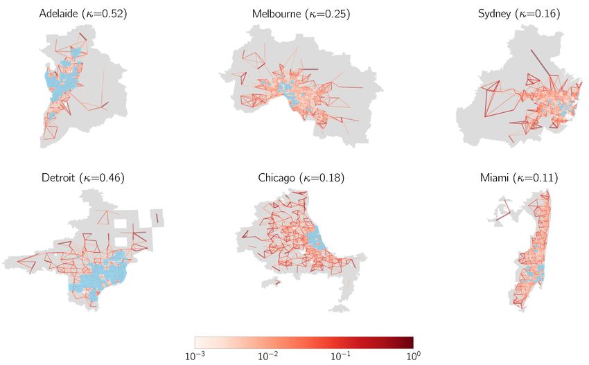
In Fig. 3A we plot the empirically extracted growth rate b as a function of the epidemic
threshold, λc , finding once again an inverse trend, confirming the role of the threshold as a
proxy for vulnerability. Those cities which experienced a faster epidemic growth during the
early onset of the pandemic indeed had a lower threshold according to our formalism.
110.45 New York
Bos
0.45 New York
0.25 rP = −0.62
Mia rS = −0.62
0.40 0.20
Phi
0.40
0.15
0.35 0.35
City vulnerability b
City vulnerability b
0.10 rP = 0.83
0.30 0.55 0.60 0.65 0.70 0.75 0.30 rS = 0.53
Boston Boston
rP = −0.66
0.25 rS = −0.65
0.25 Miami Bos
Miami Philadelphia
0.25 Mia
Phi
0.20 Philadelphia 0.20
0.20
0.15 0.15 0.15
rP = 0.60
rS = 0.50
0.10
0.10 0.10
2500 5000 7500 10000
0.55 0.60 0.65 0.70 0.75 0 10000 20000 30000
λc hdhot iκ0.43
FIG. 3. Validation of the model in US cities A Epidemic growth rate b as a function of the
epidemic threshold λc (p) (Eq. S16). In inset we show the same plot after removing NYC. B Epi-
demic growth rate b as a function of the average population density within hotspots hdhot i and the
hotspot concentration κ. The exponent 0.43 is introduced to reflect the dependence obtained when
fitting the normalized epidemic threshold to κ for the United States (Table S2). In both panels,
rP and rS denote the Pearson and Spearman rank correlation coefficients among the represented
quantities.
Next we connect, the localization of flows to hotspots to the empirical vulnerability in each
of the cities. Since κ only takes into account flows between hotspots but does not account
for their population density, the variable that captures the effective interaction between
the residents in hotspots areas should be a combination of both factors. Specifically, we
have chosen hdhot iκ0.43 , where the first term corresponds to the average population density
within hotspots and the second term reflects the scaling obtained for the normalized epidemic
threshold in the individual case of CBSA from the United States (see Supplementary Section
4 for further details). In Fig. 3B we plot b as a function of this quantity finding a clear
monotonically increasing trend. Thus taken together, the results of Fig. 3 indicate that
the empirical trends mirror our theoretical formalism, whereby cities that experience strong
early growth of the epidemic have a lower threshold, a phenomenon for which one of the main
causative mechanisms is that the movement in cities occurs primarily between hotspots.
12E. Potential mitigation measures
The observations thus far, immediately suggest the possibility of effective mitigation mea-
sures that may shore up the robustness of vulnerable cities to the onset of epidemic spread.
Given the lack of therapeutics or vaccines for SARS-COV-2, the prevailing strategy adopted
globally has been to resort to non-pharmaceutical interventions of which a key ingredient
has been aggressive lock-downs. While ostensibly being very effective in mitigating an ac-
tive epidemic, significant disruption to the socio-economic fabric is one of the unfortunate
consequences [58, 59]. Having demonstrated the key role played by the interactions be-
tween population density hotspots, we next investigate some targeted interventions, or even
preemptions, that are milder than completely restricting mobility city-wide and assess their
efficacy in reducing vulnerability. The strategy we pursue is to modify flows between different
types of locations in the city without the need to isolate individuals at home. The different
schemes are illustrated in the upper panel of Fig. 4. In the first intervention (Intervention
I), an asymmetrical strategy involves restricting flows from non-hotspot (heretofore referred
to as suburbs) towards hotspot areas and converting them to self-loops, while keeping all
other flows the same. Intervention II corresponds to the reverse situation where flows from
hotspots to suburbs are converted to self-loops. Finally, in Intervention III, only movement
between hotspots is restricted.
For each of these scenarios we recompute the normalized epidemic threshold λ̃m c (m ∈
{I,II,III}) and plot it against the original threshold, λ˜c , in the bottom panels of Fig. 4.
In panel A, we find an increase of the threshold across the board indicating that Interven-
tion I is a rather effective strategy. Given that a potential epidemic has a high probability
of being seeded and correspondingly spreading extensively in high population density ar-
eas, preventing the residents in suburbs from visiting these locations protects them from
being exposed to the disease. Conversely in panel B we see that restricting residents in
hotspots to travel to suburbs has the opposite effect in further decreasing the threshold.
This counterproductive effect emerges due to a phenomenon discussed in [28]. When there
is an asymmetry between the population density in cities, mobility from hotspots to suburbs
13A B C
Intervention I Intervention II Intervention III
Suburb
Hotspot
0.5
5 5 5
0.4
4 4 4
0.3
3 3 3
˜ III
˜ II
˜ Ic
c
c
0.2
2 2 2
0.1
1 1 1
0.0
1 2 3 4 5 1 2 3 4 5 1 2 3 4 5
˜c ˜c ˜c
FIG. 4. Impact of mobility interventions on the epidemic threshold within cities in
the United States. The impact is quantified by representing the normalized threshold for each
intervention, λ̃Ic , λ̃II III (in panels A,B,C respectively) as a function of the normalized threshold
c , λ̃c
λ̃c . In all panels, the dashed line denotes the boundary separating the cities for which the inter-
vention is beneficial (above) or detrimental (below). The color of the points represent the hotspot
concentration κ for each CBSA.
leads to an increase in the threshold due to the dilution of the effective population in the
hotspots thus reducing the number of contacts, as well as diverting potentially infectious
individuals to to lower density regions where their impact is mitigated. Removing this route
makes the situation significantly worse. Finally, panel C reveals that limiting the mobility
between hotspots has a mostly neutral effect, although the trends are noisier given that
its effectiveness is closely related to the underlying population density distribution inside
hotspots. The results suggest that, among the scenarios outlined, the most beneficial policy
is to restrict residents in suburbs from visiting hotspots, while at the same time allowing
residents in hotspots to continue with their regular mobility behavior. Note, that several
other combinations are possible, for instance a combination of interventions I & III which is
likely to have even more of a beneficial effect.
14III. Discussion
Similar to how a virus enters the human body and replicates from cell to cell, the spread
of pathogens in susceptible populations is influenced by the interaction between its hosts.
Thus, it is the social interactions, mediated by behavioral and mixing patterns, that shapes
the spread of disease in human populations. Among these aspects, human mobility is a
key factor underlying the unfolding patterns of epidemic outbreaks. Understanding how
human mobility shapes the spatiotemporal unfolding of contagious diseases is essential for
the design of efficient containment policies to ameliorate their impact. In this paper, we
investigate the interplay between the population density and the spatial distribution of flows
in urban areas, and its impact on determining exposure to epidemic outbreaks. We report
a clear trend worldwide: the existence of a high volume of individuals commuting among
the population density centers of a given city makes it more vulnerable to the spread of
epidemics. The extent of a city’s vulnerability as determined from our formalism, allows
us to shed light on a real epidemic scenario: the spread of SARS-COV-2 across United
States. In particular, the epidemic threshold determined by the population density profiles
and urban mobility patterns provides one of the potential causative mechanisms behind the
different levels of infection observed across cities in the United States.
As an application to potential epidemic waves, our indicator allows for identifying those cities
that are likely to become epidemic centers once the first imported cases arrive there. This is
of importance, given that it can guide authorities to identify places where timely containment
policies can be locally implemented to avoid large outbreaks caused by massive community
transmission. It is precisely the lack of anticipation to the SARS-COV-2 pandemic, that has
led countries to enforce aggressive containment measures aimed at ameliorating the impact
of the disease. The predominant strategy has been the implementation of lockdown policies,
forcing a large fraction of the population to stay isolated at home, thus reducing consid-
erably their number of interactions. While there is consensus on the effectiveness of these
interventions to mitigate an ongoing outbreak, the collateral socio-economic damage caused
by lockdowns requires a change of direction towards less-aggressive containment measures.
15In the case of SARS-COV-2, the strict individual isolation characterizing the first interven-
tions have given rise to more relaxed lockdown scenarios combined with efficient Test-Track
and Isolate policies [60–62]. Along these lines, we present different realistic scenarios based
on modifying mobility habits to actively avoid the emergence of large areas of contagion.
Our analysis suggest that a potentially effective policy involves an asymmetric closure of
neuralgic centers of the cities, restricting movement to population density hotspots from res-
idents of other areas, while allowing those living in hotspots to commute, in order to dilute
the number of contacts in the most vulnerable areas. Teleworking and effective distribution
of key services in a city are practical manifestations of such interventions.
An advantage of our formalism is its relative simplicity, paving the way to extend the results
to more general scenarios. For example, these results are built upon the assumption that
population density centers are much more vulnerable to contagious diseases than scarcely
dense areas. While this is a logical assumption, the beneficial effect of mobility from hotspots
and suburbs could be reversed for diseases with large reproduction number R0 . In this
scenario, suburbs would also have the potential to develop large outbreaks so the existence
of infection routes across the city would lead to an acceleration of the propagation of the
epidemic front. Finally, another obvious extension is to consider movement at different
geographical scales [63, 64]. Accounting for movement between cities, for instance, could
provide valuable information to coordinate joint efforts among different regions to modify
both inter- and intra-urban flows in service of reducing the impact of a pandemic. Needless
to say, pandemics are complex processes involving a multitude of spatial and socioeconomic
factors. The results presented here may provide one of the building blocks for policy planners
in devising effective preventive and mitigation measures for future crises.
Limitations
These results should be interpreted in light of several important limitations. First, the Google
mobility data is limited to smartphone users who have opted in to Google’s Location History
feature, which is off by default. These data may not be representative of the population as
whole, and furthermore their representativeness may vary by location. Importantly, these
limited data are only viewed through the lens of differential privacy algorithms, specifically
16designed to protect user anonymity and obscure fine detail. Moreover, comparisons across
rather than within locations are only descriptive since these regions can differ in substantial
ways.
[1] The world of air transport in 2018. Tech. Rep., International Civil Aviation Organization
(2018).
[2] Varghese, N. Globalization of higher education and cross-border student mobility (Citeseer,
2008).
[3] Filatotchev, I., Liu, X., Lu, J. & Wright, M. Knowledge spillovers through human mobility
across national borders: Evidence from zhongguancun science park in china. Research Policy
40, 453–462 (2011).
[4] Williams, A. M. & Baláž, V. What human capital, which migrants? returned skilled migration
to slovakia from the uk 1. International migration review 39, 439–468 (2005).
[5] Boubtane, E., Dumont, J.-C. & Rault, C. Immigration and economic growth in the oecd
countries 1986–2006. Oxford Economic Papers 68, 340–360 (2016).
[6] United Nations, Department of Economic and Social Affairs, Population Division (2019).
World Urbanization Prospects 2018: Highlights (ST/ESA/SER.A/421). https://
population.un.org/wup/Publications/Files/WUP2018-Highlights.pdf. Accessed: 2019-
01-30.
[7] Le Néchet, F. Urban spatial structure, daily mobility and energy consumption: a study of 34
european cities. Cybergeo: European Journal of Geography 580 (2012).
[8] Bettencourt, L. M. The origins of scaling in cities. Science 340, 1438–1441 (2013).
[9] Pan, W., Ghoshal, G., Krumme, C., Cebrian, M. & Pentland, A. Urban characteristics
attributable to density-driven tie formation. Nature Communications 4, 1961 (2013).
[10] Kirkley, A., Barbosa, H., Barthelemy, M. & Ghoshal, G. From the betweenness centrality in
street networks to structural invariants in random planar graphs. Nature Communications 9,
2501 (2018).
17[11] Van Kerkhove, M. D. et al. Epidemiologic and virologic assessment of the 2009 influenza
a (h1n1) pandemic on selected temperate countries in the southern hemisphere: Argentina,
australia, chile, new zealand and south africa. Influenza and other respiratory viruses 5,
e487–e498 (2011). URL https://pubmed.ncbi.nlm.nih.gov/21668677.
[12] Gomes, M. F. et al. Assessing the international spreading risk associated with the 2014 west
african ebola outbreak. PLoS currents 6 (2014).
[13] Zhang, Q. et al. Spread of zika virus in the americas. Proceedings of the National Academy of
Sciences 114, E4334–E4343 (2017).
[14] Estrada, E. Covid-19 and sars-cov-2. modeling the present, looking at the future. Physics
Reports 869, 1–51 (2020).
[15] Organization, W. H. et al. Coronavirus disease 2019 (covid-19): situation report, 72. Tech.
Rep. (2020).
[16] Saunders-Hastings, P. R. & Krewski, D. Reviewing the history of pandemic influenza: Under-
standing patterns of emergence and transmission. Pathogens 5, 66 (2016).
[17] Bowen Jr, J. T. & Laroe, C. Airline networks and the international diffusion of severe acute
respiratory syndrome (sars). Geographical Journal 172, 130–144 (2006).
[18] Brockmann, D. & Helbing, D. The Hidden Geometry of Complex, Network-Driven Contagion
Phenomena. Science 342, 1337 LP – 1342 (2013). URL http://science.sciencemag.org/
content/342/6164/1337.abstract.
[19] Colizza, V., Barrat, A., Barthélemy, M. & Vespignani, A. Predictability and epidemic path-
ways in global outbreaks of infectious diseases: the sars case study. BMC Medicine 5, 34
(2007). URL https://doi.org/10.1186/1741-7015-5-34.
[20] Lemey, P., Hong, S., Hill, V. & et al. Accommodating individual travel history and unsampled
diversity in bayesian phylogeographic inference of sars-cov-2. Nature Communications 11, 5110
(2020).
[21] Barbosa, H. et al. Human mobility: Models and applications. Physics Reports 734, 1–74
(2018). URL http://www.sciencedirect.com/science/article/pii/S037015731830022X.
[22] Bonaccorsi, G. et al. Economic and social consequences of human mobility restrictions under
covid-19. Proceedings of the National Academy of Sciences 117, 15530–15535 (2020).
18[23] Ahmed, F., Ahmed, N., Pissarides, C. & Stiglitz, J. Why inequality could spread covid-19.
The Lancet Public Health 5, e240 (2020).
[24] Pastor-Satorras, R., Castellano, C., Van Mieghem, P. & Vespignani, A. Epidemic processes
in complex networks. Reviews of Modern Physics 87, 925–979 (2015). URL https://link.
aps.org/doi/10.1103/RevModPhys.87.925.
[25] Belik, V., Geisel, T. & Brockmann, D. Natural Human Mobility Patterns and Spatial Spread
of Infectious Diseases. Physical Review X 1, 011001 (2011). URL https://link.aps.org/
doi/10.1103/PhysRevX.1.011001.
[26] Balcan, D. & Vespignani, A. Phase transitions in contagion processes mediated by recurrent
mobility patterns. Nature Physics 7, 581–586 (2011). URL https://doi.org/10.1038/
nphys1944.
[27] Gómez-Gardeñes, J., Soriano-Paños, D. & Arenas, A. Critical regimes driven by recurrent
mobility patterns of reaction–diffusion processes in networks. Nature Physics 14, 391–395
(2018). URL https://doi.org/10.1038/s41567-017-0022-7.
[28] Soriano-Paños, D., Lotero, L., Arenas, A. & Gómez-Gardeñes, J. Spreading Processes in
Multiplex Metapopulations Containing Different Mobility Networks. Physical Review X 8,
031039 (2018). URL https://link.aps.org/doi/10.1103/PhysRevX.8.031039.
[29] Moss, R., Naghizade, E., Tomko, M. & Geard, N. What can urban mobility data reveal about
the spatial distribution of infection in a single city? BMC Public Health 19, 656 (2019). URL
https://doi.org/10.1186/s12889-019-6968-x.
[30] Granell, C. & Mucha, P. J. Epidemic spreading in localized environments with recurrent
mobility patterns. Physical Review E 97, 052302 (2018).
[31] Soriano-Paños, D., Ghoshal, G., Arenas, A. & Gómez-Gardeñes, J. Impact of temporal scales
and recurrent mobility patterns on the unfolding of epidemics. Journal of Statistical Mechanics:
Theory and Experiment 2020, 024006 (2020). URL https://iopscience.iop.org/article/
10.1088/1742-5468/ab6a04.
[32] Tizzoni, M. et al. On the use of human mobility proxies for modeling epidemics. PLOS
Computational Biology 10, 1–15 (2014). URL https://doi.org/10.1371/journal.pcbi.
1003716.
19[33] Mazzoli, M. et al. Field theory for recurrent mobility. Nature Communications 10, 3895
(2019).
[34] Barbosa, H., de Lima-Neto, F. B., Evsukoff, A. & Menezes, R. The effect of recency to human
mobility. EPJ Data Science 4, 21 (2015).
[35] Soriano-Paños, D. et al. Vector-borne epidemics driven by human mobility. Physical Review
Research 2, 013312 (2020).
[36] Tizzoni, M. et al. Real-time numerical forecast of global epidemic spreading: case study
of 2009 a/h1n1pdm. BMC Medicine 10, 165 (2012). URL https://doi.org/10.1186/
1741-7015-10-165.
[37] Wesolowski, A. et al. Quantifying the impact of human mobility on malaria. Science 338,
267–270 (2012).
[38] Arenas, A. et al. A mathematical model for the spatiotemporal epidemic spreading of
COVID19. medRxiv 2020.03.21.20040022 (2020). URL https://www.medrxiv.org/content/
10.1101/2020.03.21.20040022v1.
[39] Costa, G. S., Cota, W. & Ferreira, S. C. Metapopulation modeling of COVID-19 advancing into
the countryside: an analysis of mitigation strategies for Brazil. medRxiv 2020.05.06.20093492
(2020). URL https://www.medrxiv.org/content/10.1101/2020.05.06.20093492v2.
[40] Badr, H. S. et al. Association between mobility patterns and covid-19 transmission in the usa:
a mathematical modelling study. The Lancet Infectious Diseases .
[41] Bertuzzo, E. et al. The geography of covid-19 spread in italy and implications for the relaxation
of confinement measures. Nature Communications 11, 4264 (2020).
[42] Alirol, E., Getaz, L., Stoll, B., Chappuis, F. & Loutan, L. Urbanisation and infectious diseases
in a globalised world. The Lancet. Infectious diseases 11, 131–141 (2011). URL https:
//pubmed.ncbi.nlm.nih.gov/21272793.
[43] Kraemer, M. U. G. et al. Big city, small world: density, contact rates, and transmission
of dengue across pakistan. Journal of the Royal Society, Interface 12, 20150468–20150468
(2015). URL https://pubmed.ncbi.nlm.nih.gov/26468065.
[44] Li, R., Richmond, P. & Roehner, B. M. Effect of population density on epidemics. Physica A:
Statistical Mechanics and its Applications 510, 713–724 (2018). URL https://EconPapers.
20repec.org/RePEc:eee:phsmap:v:510:y:2018:i:c:p:713-724.
[45] Lee, M., Barbosa, H., Youn, H., Holme, P. & Ghoshal, G. Morphology of travel routes and
the organization of cities. Nature Communications 8, 2229 (2017).
[46] Bassolas, A. et al. Hierarchical organization of urban mobility and its connection with
city livability. Nature Communications 10, 4817 (2019). URL https://doi.org/10.1038/
s41467-019-12809-y.
[47] Louail, T. et al. From mobile phone data to the spatial structure of cities. Scientific Reports
4, 5276 (2014). URL https://doi.org/10.1038/srep05276.
[48] Free US Population Density And Unemployment Rate By Zip Code (ac-
cessed 2020- 08-27). URL https://blog.splitwise.com/2014/01/06/
free-us-population-density-and-unemployment-rate-by-zip-code/.
[49] Australian Bureau of Statistics. https://www.abs.gov.au/.
[50] Statistics South Africa. http://www.statssa.gov.za.
[51] Facebook (accessed 2020- 08-27). URL https://data.humdata.org/organization/
facebook.
[52] Rader, B. et al. Crowding and the shape of covid-19 epidemics. Nature Medicine (2020).
[53] Di Domenico, L., Pullano, G., Sabbatini, C. E., Boëlle, P.-Y. & Colizza, V. Impact of lockdown
on covid-19 epidemic in ı̂le-de-france and possible exit strategies. BMC Medicine 18, 240
(2020).
[54] Prem, K. et al. The effect of control strategies to reduce social mixing on outcomes of the
covid-19 epidemic in wuhan, china: a modelling study. The Lancet Public Health (2020).
[55] Gatto, M. et al. Spread and dynamics of the covid-19 epidemic in italy: Effects of emergency
containment measures. Proceedings of the National Academy of Sciences 117, 10484–10491
(2020).
[56] https://github.com/nytimes/covid-19-data.
[57] https://usafacts.org/visualizations/coronavirus-covid-19-spread-map/.
[58] Gdp and employment flash estimates for the second quarter of 2020. Tech. Rep., Eurostat
(2020).
[59] Gross domestic product, second quarter 2020 (advance estimate) and annual update. Tech.
21Rep., Bureau of Economic Analysis (2020).
[60] Hellewell, J. et al. Feasibility of controlling covid-19 outbreaks by isolation of cases and
contacts. The Lancet Global Health (2020).
[61] Ferretti, L. et al. Quantifying sars-cov-2 transmission suggests epidemic control with digital
contact tracing. Science 368 (2020).
[62] Salathé, M. et al. Covid-19 epidemic in switzerland: on the importance of testing, contact
tracing and isolation. Swiss medical weekly 150, w20225 (2020).
[63] Watts, D. J., Muhamad, R., Medina, D. C. & Dodds, P. S. Multiscale, resurgent epidemics in
a hierarchical metapopulation model. Proceedings of the National Academy of Sciences 102,
11157–11162 (2005).
[64] Balcan, D. et al. Multiscale mobility networks and the spatial spreading of infectious diseases.
Proceedings of the National Academy of Sciences 106, 21484–21489 (2009).
[65] Wilson, R. et al. Differentially private sql with bounded user contribution (2020).
[66] Https://research.google/pubs/pub48778/.
[67] Hu, H., Nigmatulina, K. & Eckhoff, P. The scaling of contact rates with population density
for the infectious disease models. Mathematical Biosciences 244, 125 – 134 (2013). URL
http://www.sciencedirect.com/science/article/pii/S0025556413001235.
[68] https://github.com/nytimes/covid-19-data.
[69] https://usafacts.org/visualizations/coronavirus-covid-19-spread-map/.
[70] Savitzky–Golay filter (accessed 2020- 08-17). URL https://en.wikipedia.org/wiki/
Savitzky-Golay_filter.
[71] Smoothing in Python (accessed 2020- 08-17). URL https://plotly.com/python/
smoothing/.
22Supporting Information
S1. Hotspot classification
Hotspots are identified by setting a threshold on the population densities of cells within
a city. The threshold for hotspots is assigned by applying a non-parametric method, the
LouBar method [46, 47], based on the derivative of the Lorenz curve. The Lorenz curve is
the sorted cumulative distribution of population densities and is obtained by plotting, in
ascending order, the normalized cumulative number of nodes vs. the normalized cumulative
population density. The threshold is then obtained by taking the derivative of the Lorenz
curve at (1, 1) and extrapolating it to the point at which it intersects the x-axis. We
classify hotspots in cities according to this LouBar method applied to population densities,
in agreement with the reliance of the model on effective densities. A cell i is considered a
hotspot of city k, Hk if it satisfies:
di,k > dLou
k (S1)
where di is the population density of cell i in city k and dLou
k is the threshold determined by
performing the LouBar method on the population densities of all cells in city k. This allows
us to place emphasis on zones within cities that encourage the most relative interaction, as
opposed to sharp biasing due to population magnitude. We then examine the hotspots flow
concentration in each city k, κk , defined as fraction of total flows in the city system that
exist between these population density hotspots of city. Therefore, κk is given by:
P
Tij
i,jHk
κk = P , (S2)
Tij
i,j
where Tij denotes the flow of individuals going from patch i to patch j according to the
mobility data.
S-1S2. Data
TABLE S1: Hotspot flow concentration κ for the different
cities analyzed in the manuscript. The resolution column con-
tain the two geographical divisions used inside each country
to construct the metapopulations. For example, “Zip codes
within CBSA” in the case of the USA implies that each city
(metapopulation) corresponds to a CBSA and the entities
composing each city (patches) correspond to zip codes.
City Country Resolution κ
Bunbury AUS SA2 within SA4 0.059
Capital Region AUS SA2 within SA4 0.125
Sydney AUS SA2 within SA4 0.162
Darwin AUS SA2 within SA4 0.185
Cairns AUS SA2 within SA4 0.186
Richmond AUS SA2 within SA4 0.202
Gold Coast AUS SA2 within SA4 0.212
South Australia AUS SA2 within SA4 0.221
Hume AUS SA2 within SA4 0.228
Moreton Bay AUS SA2 within SA4 0.233
Central Queensland AUS SA2 within SA4 0.236
Wide Bay AUS SA2 within SA4 0.237
Melbourne AUS SA2 within SA4 0.250
Townsville AUS SA2 within SA4 0.250
Australian Capital Territory AUS SA2 within SA4 0.253
Launceston and North East AUS SA2 within SA4 0.303
Sunshine Coast AUS SA2 within SA4 0.308
S-2City Country Resolution κ
Central Coast AUS SA2 within SA4 0.310
Illawarra AUS SA2 within SA4 0.325
Perth AUS SA2 within SA4 0.330
Logan AUS SA2 within SA4 0.349
Brisbane AUS SA2 within SA4 0.350
Hunter Valley exc Newcastle AUS SA2 within SA4 0.369
Newcastle and Lake Macquarie AUS SA2 within SA4 0.381
Western Australia AUS SA2 within SA4 0.386
Ipswich AUS SA2 within SA4 0.396
West and North West AUS SA2 within SA4 0.415
Mackay AUS SA2 within SA4 0.415
Latrobe AUS SA2 within SA4 0.419
North West AUS SA2 within SA4 0.423
Hobart AUS SA2 within SA4 0.438
Central West AUS SA2 within SA4 0.496
Adelaide AUS SA2 within SA4 0.520
Bolzano ITA S2 cells within communes 0.210
Sassari ITA S2 cells within communes 0.278
Catania ITA S2 cells within communes 0.300
Livorno ITA S2 cells within communes 0.306
Taranto ITA S2 cells within communes 0.307
Foggia ITA S2 cells within communes 0.318
Perugia ITA S2 cells within communes 0.319
Bari ITA S2 cells within communes 0.337
Giugliano In Campania ITA S2 cells within communes 0.337
Terni ITA S2 cells within communes 0.341
Piacenza ITA S2 cells within communes 0.344
S-3City Country Resolution κ
Genova ITA S2 cells within communes 0.376
Ravenna ITA S2 cells within communes 0.381
Ferrara ITA S2 cells within communes 0.392
Ancona ITA S2 cells within communes 0.392
Lecce ITA S2 cells within communes 0.393
Cesena ITA S2 cells within communes 0.394
Pesaro ITA S2 cells within communes 0.405
Parma ITA S2 cells within communes 0.406
Pescara ITA S2 cells within communes 0.434
Roma ITA S2 cells within communes 0.435
Venezia ITA S2 cells within communes 0.436
Modena ITA S2 cells within communes 0.458
Trieste ITA S2 cells within communes 0.466
Brescia ITA S2 cells within communes 0.467
Trento ITA S2 cells within communes 0.469
Siracusa ITA S2 cells within communes 0.470
Napoli ITA S2 cells within communes 0.471
Palermo ITA S2 cells within communes 0.472
Milano ITA S2 cells within communes 0.478
Rimini ITA S2 cells within communes 0.479
Prato ITA S2 cells within communes 0.489
Verona ITA S2 cells within communes 0.494
Salerno ITA S2 cells within communes 0.501
Torino ITA S2 cells within communes 0.507
Arezzo ITA S2 cells within communes 0.527
Reggio Di Calabria ITA S2 cells within communes 0.534
Latina ITA S2 cells within communes 0.543
S-4City Country Resolution κ
Udine ITA S2 cells within communes 0.545
Bologna ITA S2 cells within communes 0.567
Vicenza ITA S2 cells within communes 0.568
Andria ITA S2 cells within communes 0.575
Novara ITA S2 cells within communes 0.582
Padova ITA S2 cells within communes 0.586
Bergamo ITA S2 cells within communes 0.598
Firenze ITA S2 cells within communes 0.629
Messina ITA S2 cells within communes 0.657
Cagliari ITA S2 cells within communes 0.751
Monza ITA S2 cells within communes 0.773
Virginia Beach USA Zip codes within CBSA 0.033
Washington USA Zip codes within CBSA 0.104
Miami USA Zip codes within CBSA 0.109
Columbus USA Zip codes within CBSA 0.140
Seattle USA Zip codes within CBSA 0.140
Atlanta USA Zip codes within CBSA 0.157
Houston USA Zip codes within CBSA 0.170
Pittsburgh USA Zip codes within CBSA 0.178
Richmond USA Zip codes within CBSA 0.180
Raleigh USA Zip codes within CBSA 0.182
San Francisco USA Zip codes within CBSA 0.184
Nashville USA Zip codes within CBSA 0.188
Los Angeles USA Zip codes within CBSA 0.189
Salt Lake City USA Zip codes within CBSA 0.204
Cincinnati USA Zip codes within CBSA 0.205
New York USA Zip codes within CBSA 0.213
S-5City Country Resolution κ
Austin USA Zip codes within CBSA 0.213
Minneapolis USA Zip codes within CBSA 0.215
Birmingham USA Zip codes within CBSA 0.220
Boston USA Zip codes within CBSA 0.229
Providence USA Zip codes within CBSA 0.231
Charlotte USA Zip codes within CBSA 0.235
Louisville/Jefferson County USA Zip codes within CBSA 0.246
Dallas USA Zip codes within CBSA 0.247
Orlando USA Zip codes within CBSA 0.252
St. Louis USA Zip codes within CBSA 0.256
Riverside USA Zip codes within CBSA 0.269
Buffalo USA Zip codes within CBSA 0.270
Chicago USA Zip codes within CBSA 0.276
Kansas City USA Zip codes within CBSA 0.286
Baltimore USA Zip codes within CBSA 0.292
San Jose USA Zip codes within CBSA 0.295
Denver USA Zip codes within CBSA 0.297
Philadelphia USA Zip codes within CBSA 0.298
Cleveland USA Zip codes within CBSA 0.304
Hartford USA Zip codes within CBSA 0.316
San Antonio USA Zip codes within CBSA 0.327
Portland USA Zip codes within CBSA 0.349
San Diego USA Zip codes within CBSA 0.352
Phoenix USA Zip codes within CBSA 0.383
Milwaukee USA Zip codes within CBSA 0.385
Memphis USA Zip codes within CBSA 0.393
Indianapolis USA Zip codes within CBSA 0.411
S-6City Country Resolution κ
Las Vegas USA Zip codes within CBSA 0.415
Oklahoma City USA Zip codes within CBSA 0.418
Sacramento USA Zip codes within CBSA 0.419
New Orleans USA Zip codes within CBSA 0.424
Jacksonville USA Zip codes within CBSA 0.436
Tampa USA Zip codes within CBSA 0.436
Detroit USA Zip codes within CBSA 0.462
Govan Mbeki ZAF Wards within municipalities 0.013
Hibiscus Coast ZAF Wards within municipalities 0.023
City of Matlosana ZAF Wards within municipalities 0.025
Nelson Mandela Bay ZAF Wards within municipalities 0.028
City of Cape Town ZAF Wards within municipalities 0.029
Emalahleni ZAF Wards within municipalities 0.031
City of Tshwane ZAF Wards within municipalities 0.033
Local Municipality of Madibeng ZAF Wards within municipalities 0.041
Ekurhuleni ZAF Wards within municipalities 0.044
City of Johannesburg ZAF Wards within municipalities 0.054
Matjhabeng ZAF Wards within municipalities 0.060
Nkomazi ZAF Wards within municipalities 0.060
Greater Letaba ZAF Wards within municipalities 0.064
Mangaung ZAF Wards within municipalities 0.069
Makhado ZAF Wards within municipalities 0.075
Emfuleni ZAF Wards within municipalities 0.107
Greater Tzaneen ZAF Wards within municipalities 0.137
eThekwini ZAF Wards within municipalities 0.147
Mogalakwena ZAF Wards within municipalities 0.149
Lepele ZAF Wards within municipalities 0.151
S-7City Country Resolution κ
Buffalo City ZAF Wards within municipalities 0.216
Polokwane ZAF Wards within municipalities 0.244
The Msunduzi ZAF Wards within municipalities 0.247
Rustenburg ZAF Wards within municipalities 0.253
Makhuduthamaga ZAF Wards within municipalities 0.265
Thembisile ZAF Wards within municipalities 0.285
Chief Albert Luthuli ZAF Wards within municipalities 0.465
Dr JS Moroka ZAF Wards within municipalities 0.497
Maluti a Phofung ZAF Wards within municipalities 0.502
Bushbuckridge ZAF Wards within municipalities 0.580
Thulamela ZAF Wards within municipalities 0.645
A. Mobility Data
The Google COVID-19 Aggregated Mobility Research Dataset contains anonymized mobility
flows aggregated over users who have turned on the Location History setting, which is off
by default. This is similar to the data used to show how busy certain types of places are in
Google Maps — helping identify when a local business tends to be the most crowded. The
dataset aggregates flows of people from region to region.
To produce this dataset, machine learning is applied to logs data to automatically segment
it into semantic trips [46]. To provide strong privacy guarantees, all trips were anonymized
and aggregated using a differentially private mechanism [65] to aggregate flows over time (see
https://policies.google.com/technologies/anonymization). This research is done on
the resulting heavily aggregated and differentially private data. No individual user data was
ever manually inspected, only heavily aggregated flows of large populations were handled.
All anonymized trips are processed in aggregate to extract their origin and destination loca-
tion and time. For example, if users traveled from location a to location b within time interval
S-8You can also read