Buoyant calving and ice-contact lake evolution at Pasterze Glacier (Austria) in the period 1998-2019 - The Cryosphere
←
→
Page content transcription
If your browser does not render page correctly, please read the page content below
The Cryosphere, 15, 1237–1258, 2021
https://doi.org/10.5194/tc-15-1237-2021
© Author(s) 2021. This work is distributed under
the Creative Commons Attribution 4.0 License.

Buoyant calving and ice-contact lake evolution at Pasterze Glacier
(Austria) in the period 1998–2019
Andreas Kellerer-Pirklbauer1 , Michael Avian2 , Douglas I. Benn3 , Felix Bernsteiner1 , Philipp Krisch1 , and
Christian Ziesler1
1 Cascade – The mountain processes and mountain hazards group, Institute of Geography and Regional Science,
University of Graz, Graz, Austria
2 Department of Earth Observation, Zentralanstalt für Meteorologie und Geodynamik (ZAMG), Vienna, Austria
3 School of Geography and Sustainable Development, University of St Andrews, St Andrews, UK

Correspondence: Andreas Kellerer-Pirklbauer (andreas.kellerer@uni-graz.at)

Received: 9 August 2020 – Discussion started: 18 September 2020
Revised: 27 January 2021 – Accepted: 30 January 2021 – Published: 10 March 2021

Abstract. Rapid growth of proglacial lakes in the current         by ablation of glacier ice and debris-covered dead ice form-
warming climate can pose significant outburst flood hazards,      ing thermokarst features; increase in hydrostatic disequilib-
increase rates of ice mass loss, and alter the dynamic state      rium leading to destabilization of ice at the lake bottom or
of glaciers. We studied the nature and rate of proglacial lake    at the near-shore causing fracturing, tilting, disintegration, or
evolution at Pasterze Glacier (Austria) in the period 1998–       emergence of new icebergs due to buoyant calving; and grad-
2019 using different remote-sensing (photogrammetry, laser        ual melting of icebergs along with iceberg capsizing events.
scanning) and fieldwork-based (global navigation satellite        We conclude that buoyant calving, previously not reported
system – GNSS, time-lapse photography, geoelectrical resis-       from the European Alps, might play an important role at
tivity tomography – ERT, and bathymetry) data. Glacier thin-      alpine glaciers in the future as many glaciers are expected
ning below the spillway level and glacier recession caused        to recede into valley or cirque overdeepenings.
flooding of the glacier, initially forming a glacier-lateral
to supraglacial lake with subaerial and subaquatic debris-
covered dead-ice bodies. The observed lake size increase in
1998–2019 followed an exponential curve (1998 – 1900 m2 ,         1   Introduction
2019 – 304 000 m2 ). ERT data from 2015 to 2019 revealed
widespread existence of massive dead-ice bodies exceeding         Ongoing recession of mountain glaciers worldwide reveals
25 m in thickness near the lake shore. Several large-scale and    dynamic landscapes exposed to high rates of geomorpho-
rapidly occurring buoyant calving events were detected in the     logical and hydrological changes (Carrivick and Heckmann,
48 m deep basin by time-lapse photography, indicating that        2017). In suitable topographic conditions, proglacial lakes
buoyant calving is a crucial process for the fast lake expan-     may form, including ice-contact lakes (physically attached to
sion. Estimations of the ice volume losses by buoyant calving     an ice margin) and ice-marginal lakes (lakes detached from
and by subaerial ablation at a 0.35 km2 large lake-proximal       or immediately beyond a contemporary ice margin) (Benn
section of the glacier reveal comparable values for both pro-     and Evans, 2010; Carrivick and Tweed, 2013). Such lakes
cesses (ca. 1 × 10⁶ m3 ) for the period August 2018 to Au-        have increased in number, size, and volume around the world
gust 2019. We identified a sequence of processes: glacier re-     due to climate-warming-induced glacier melt (Carrivick and
cession into a basin and glacier thinning below the spillway      Tweed, 2013; Otto, 2019). Buckel et al. (2018) for instance
level; glacio-fluvial sedimentation in the glacial–proglacial     studied the formation and distribution of proglacial lakes
transition zone covering dead ice; initial formation and accel-   since the Little Ice Age (LIA) in Austria revealing a con-
erating enlargement of a glacier-lateral to supraglacial lake     tinuous acceleration in the number of glacier-related lakes
                                                                  particularly since the turn of the 21st century.

Published by Copernicus Publications on behalf of the European Geosciences Union.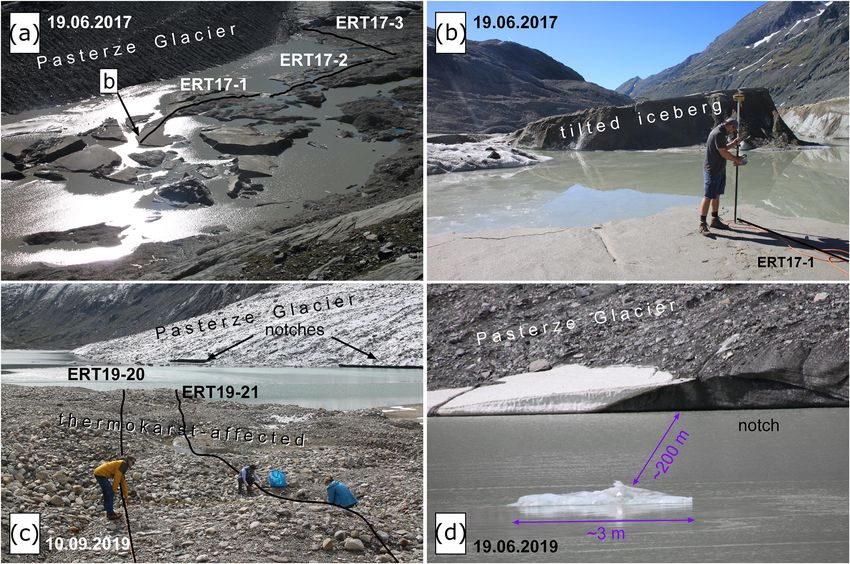
1238                     A. Kellerer-Pirklbauer et al.: Buoyant calving and ice-contact lake at Pasterze Glacier (Austria)

   The formation of proglacial lakes is important be-                 In this study, we analysed rates and processes of glacier
cause they can pose significant outburst flood hazards             recession and formation and evolution of an ice-contact lake
(e.g. Richardson and Reynolds, 2000; Harrison et al., 2018),       at Pasterze Glacier, Austria, over a period of 22 years. The
increase rates of ice mass loss, and alter the dynamic state       aims of this study are (i) to examine glaciological and mor-
of glaciers (e.g. Kirkbride and Warren, 1999; King et al.,         phological changes at the highly dynamic glacial–proglacial
2018, 2019; Liu et al., 2020). However, detailed descrip-          transition zone of the receding Pasterze Glacier and (ii) to
tions of proglacial lake formation and related subaerial and       discuss related processes which formed the proglacial lake
subaquatic processes are still rare. Carrivick and Heckmann        named Pasterzensee (See is German for lake) during the
(2017) pointed out that there is an urgent need for inventories    period 1998–2019. Regarding the latter, we focus particu-
of proglacial systems including lakes to form a baseline from      larly on the significance of buoyant calving. In doing so,
which changes could be detected.                                   we consider subaerial, subsurface, and aquatic, as well as
   The evolution of proglacial lakes is commonly linked to         subaquatic, domains applying fieldwork-based and remote-
the subsurface, particularly to changes in the distribution of     sensing techniques.
debris-covered dead ice (defined here as any part of a glacier
which has ceased to flow) and permafrost-related ground ice
bodies (Bosson et al., 2015; Gärtner-Roer and Bast, 2019)          2   Study area
affecting lake geometry and areal expansion.
                                                                   The study area comprises the glacial–proglacial transition
   Water bodies at the glacier surface form initially as
                                                                   zone of Pasterze Glacier, Austria. This glacier covered
supraglacial lakes which might be either perched lakes
                                                                   26.5 km2 during the LIA maximum in around 1850 and is the
(i.e. above the hydrological base level of the glacier) or base-
                                                                   largest glacier in the Austrian Alps with an area of 15.4 km2
level lakes (spillway controlled). The former type is prone to
                                                                   in 2019 (Fig. 1). The glacier is located in the Glockner Moun-
drainage if the perched lake connects to the englacial conduit
                                                                   tains, the Hohe Tauern range, at 47◦ 050 N, 12◦ 430 E (Fig. 1b).
system (Benn et al., 2001). Rapid areal expansion of such
                                                                   The gently sloping, 4.5 km long glacier tongue is connected
lakes is controlled by waterline and subaerial melting of ex-
                                                                   to the upper part of the glacier by an icefall named Hufeisen-
posed ice cliffs and calving (Benn et al., 2001). Furthermore,
                                                                   bruch (meaning horseshoe icefall in German) attributed to its
supraglacial lakes may transform into proglacial lakes lack-
                                                                   former shape in plan view. This icefall disintegrated and nar-
ing any ice core (full-depth lakes) through melting of lake-
                                                                   rowed substantially during the last few decades, attributed
bottom ice. However, this is a slow process in which energy
                                                                   to the decrease in ice replenishment from the upper to the
is conducted from the overlying water and cannot account for
                                                                   lower part of the glacier (Kellerer-Pirklbauer et al., 2008;
some observed instances of fast lake-bottom lowering with
                                                                   Kaufmann et al., 2015).
rates exceeding 10 m yr−1 (Thompson et al., 2012). It has
                                                                      The longest time series of length changes at Austrian
been argued that fast lake-bottom lowering could occur by
                                                                   glaciers has been compiled for Pasterze Glacier. Measure-
buoyant calving (Dykes et al., 2010; Thompson et al., 2012),
                                                                   ments at this glacier were initiated in 1879 and have been
but the rare and episodic nature of such events means that lit-
                                                                   interrupted in only three of the years since. Furthermore,
tle is known about how buoyant calving might contribute to
                                                                   annual glacier flow velocity measurements and surface ele-
the transformation of supraglacial lakes into full-depth lakes.
                                                                   vation changes at cross sections were initiated in the 1920s
   Buoyant calving occurs where ice is subject to net upward
                                                                   with almost continuous measurements since then (Lieb and
buoyant forces sufficient to overcome its tensile strength.
                                                                   Kellerer-Pirklbauer, 2018, Sect. 4.2 therein). Technical de-
Such forces can develop where either ice thinning (e.g. via
                                                                   tails of the measurement can be found in Kellerer-Pirklbauer
surface ablation) or water deepening (e.g. rises in lake level)
                                                                   et al. (2008) and Lieb and Kellerer-Pirklbauer (2018). Mi-
cause the ice to become buoyant. If the ice is unable to
                                                                   nor glacier advances at Pasterze Glacier have occurred in
adjust its geometry to achieve hydrostatic equilibrium, it
                                                                   only seven of the years since 1879, the most recent of
can become super-buoyant (Benn et al., 2007), creating ten-
                                                                   which was in the 1930s. Even during wetter and cooler peri-
sile stresses at the ice base. If these stresses become suf-
                                                                   ods (1890s, 1920s, and 1965–1980), the glacier did not ad-
ficiently high, the ice will fracture and calve, as described
                                                                   vance substantially, which can be attributed to the long re-
by Holdsworth (1973), Warren et al. (2001), and Boyce
                                                                   sponse time of the glacier (Zuo and Oerlemans, 1997). In
et al. (2007). Detailed models of super-buoyancy and buoy-
                                                                   1959–2019, Pasterze Glacier receded by 1550 m, 3 times the
ant calving have been presented by Wagner et al. (2016)
                                                                   mean value for all Austrian glaciers (520 m), related to its
and Benn et al. (2017). Hydrostatic disequilibrium caused
                                                                   large size. Today, Pasterze Glacier is characterized by annual
the sudden disintegration of debris-covered dead ice in
                                                                   mean recession rates in the order of magnitude of 40 m yr−1
the proglacial area of Pasterze Glacier in September 2016
                                                                   (Lieb and Kellerer-Pirklbauer, 2018) causing a rather high
(Fig. 2). This event was briefly described in Kellerer-
                                                                   pace of glacial to proglacial landscape modification favour-
Pirklbauer et al. (2017) and was one of the main motivations
                                                                   ing paraglacial response processes (Ballantyne, 2002; Avian
for the present study.
                                                                   et al., 2018).

The Cryosphere, 15, 1237–1258, 2021                                                   https://doi.org/10.5194/tc-15-1237-2021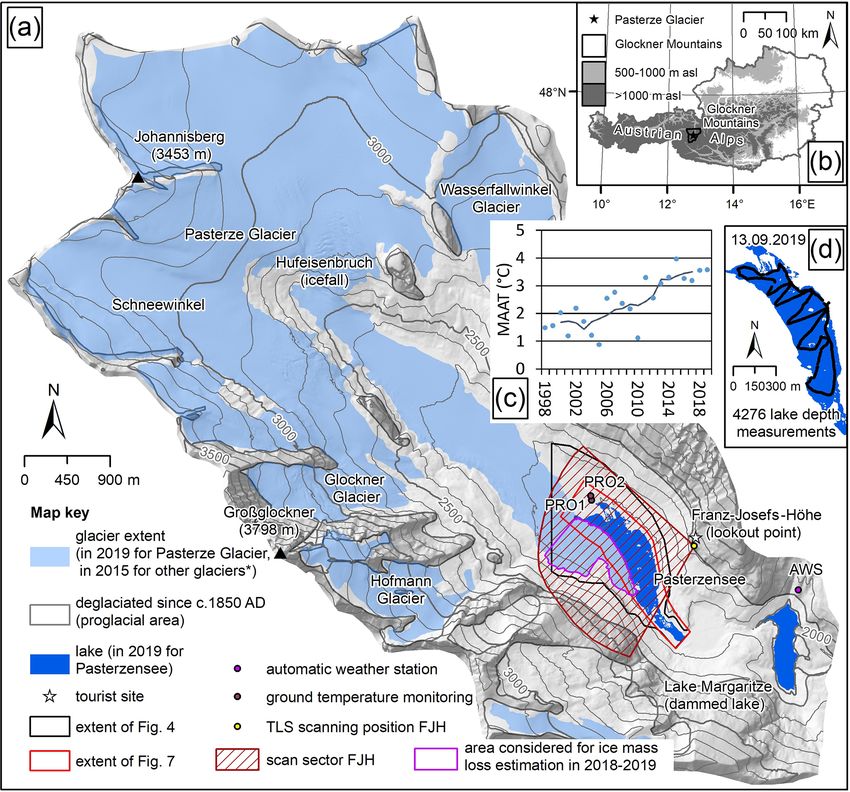
A. Kellerer-Pirklbauer et al.: Buoyant calving and ice-contact lake at Pasterze Glacier (Austria)                                        1239

Figure 1. Pasterze Glacier. (a) Location of Pasterze Glacier at the foot of Großglockner (3798 m a.s.l.). Relevant sites are indicated. (b) Lo-
cation of the study area within Austria. (c) Mean annual air temperature (MAAT) at the automatic weather station (AWS) Margaritze in
1998–2019 (single years and 5-year running mean). (d) Position of 4276 lake depth measurements carried out on 13 September 2019. Hill-
shade in the background of (a) from 2012 source KAGIS. Extent of glacier and lake in 2019 this study. Glacier extent of 2015 (*) based on
Buckel and Otto (2018). Glacier extent of ca. 1850 based on own mapping.

   Analyses of brittle and ductile structures at the surface of           tion and decrease in activity are favourable for dead ice and
the glacier tongue revealed that many of these structures are             proglacial lake formation.
relict and independent from current glacier motion (Kellerer-                An automatic weather station is located close to the study
Pirklbauer and Kulmer, 2019). The glacier tongue is in a state            area operated by VERBUND Hydro Power GmbH since
of rapid decay and thinning and thus prone to fracturing by               1982 (AWS in Fig. 1a). The coldest calendar year in the pe-
normal fault formation. Englacial and subglacial melting of               riod 1998–2019 was 2005 with a mean annual air tempera-
glacier ice caused the formation of circular collapse struc-              ture (MAAT) of 0.9 ◦ C whereas the warmest year was 2015
tures with concentric crevasses, which form when the ice                  with 4.0 ◦ C (range 3.1 ◦ C, mean of the 22-year period 2.4 ◦ C;
between the glacier surface and the roof of water channels                Fig. 1c). Interannual variation is high although a warming
decreases. Kellerer-Pirklbauer and Kulmer (2019) concluded                trend is clear. A MAAT value > 3 ◦ C was calculated for 8
that the tongue of the Pasterze Glacier is currently turning              of the 9 years between 2011 and 2019. No such high MAAT
into a large dead-ice body characterized by a strong decrease             values were recorded for the entire previous 28-year period
in ice replenishment from further up-glacier, movement ces-               1982–2010 indicating significant recent atmospheric warm-
sation, accelerated thinning and ice disintegration by supra-,            ing. Two ground temperature monitoring sites were installed
en- and subglacial ablation, allowing normal fractures and                near the lake in fluvio-glacial sediments in 2018 (PRO1 –
circular collapse features to develop. This rapid deglacia-               one sensor at the surface; PRO2 – three sensors at the sur-

https://doi.org/10.5194/tc-15-1237-2021                                                          The Cryosphere, 15, 1237–1258, 2021
1240                      A. Kellerer-Pirklbauer et al.: Buoyant calving and ice-contact lake at Pasterze Glacier (Austria)

Figure 2. Evolution of the proglacial area at Pasterze Glacier during a period of only 40 min (20 September 2016, from 09:15 to 09:55 CEST
(UTC + 2), due to loss of hydrostatic disequilibrium and buoyancy as depicted by an automatic time-lapse camera (a–e) and observed in the
field a few hours after the event (f–h). Note the sudden fracturing between 09:50 and 09:55. (a–e) Provided by GROHAG; (f–h) provided by
Konrad Mariacher, 20 September 2016. See Supplement for a related animation.

face and at 10 and 40 cm depths; for location see Fig. 1a) us-         3     Material and methods
ing a GeoPrecision data logger equipped with PT1000 tem-
perature sensors (accuracy of ±0.05 ◦ C) and logging hourly.           3.1    GNSS data
Positive mean values for a 363 d long period (13 Septem-
ber 2018–10 September 2019) were recorded for both sites               The terminus position of Pasterze Glacier was measured
(PRO1 2.6 ◦ C, PRO2 3.7–3.9 ◦ C) suggesting permafrost-free            directly in the field by global navigation satellite system
conditions in the proglacial area and unfavourable conditions          (GNSS) techniques in 14 years between 2003 and 2019 (an-
for long-term dead-ice conservation even below a protecting            nually between 2003 and 2005, in 2008, and annually be-
sediment cover.                                                        tween 2010 and 2019). Direct measurements of the subaerial
                                                                       glacier limit are essential in areas where debris cover ob-
                                                                       scures the glacier margin, hindering the successful appli-
                                                                       cation of remote-sensing techniques (e.g. Kaufmann et al.,
                                                                       2015; Avian et al., 2020). GNSS measurements were mostly

The Cryosphere, 15, 1237–1258, 2021                                                         https://doi.org/10.5194/tc-15-1237-2021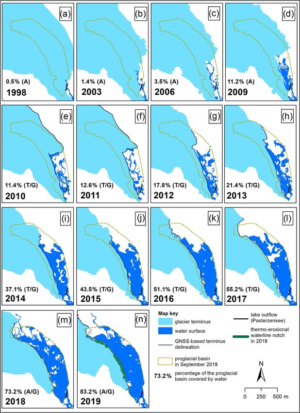
A. Kellerer-Pirklbauer et al.: Buoyant calving and ice-contact lake at Pasterze Glacier (Austria)                          1241

carried out in September of the above-listed years, thus, close   (with 1 or 0.5 m grid resolution) were calculated in Golden
to the end of the glaciological years of mid-latitude moun-       Software Surfer. In this study we used the DTMs to delin-
tain regions. Until 2013, a conventional GNSS technique was       eate the water bodies in the scan sector manually (for de-
applied using different handheld Garmin devices (geomet-          tails see Avian et al., 2020) supported by GNSS data (see
ric accuracy in the range of metres). Afterwards, a real-time     above) for the glacier boundary. In addition, the point clouds
kinematics (RTK) technique was used, where correction data        acquired by TLS were used to quantify lake-level variations
from the base station whose location is precisely known are       (see Sect. 3.4). TLS data from 2010 to 2019 (13 Septem-
transmitted to the rover (geometric accuracy in the range         ber 2010, 27 September 2011, 7 September 2012, 24 Au-
of centimetres). We utilized a Topcon HiPer V differential        gust 2013, 9 September 2014, 12 September 2015, 27 August
GPS system. Either the base station was our own local sta-        2016, 22 September 2017, 13 September 2018, and 3 August
tion (base-and-rover setup), or we obtained correction signals    2019) were analysed.
from a national correction-data provider (EPOSA, Vienna).            Furthermore, we quantified changes in ice-surface eleva-
                                                                  tion of Pasterze Glacier near the proglacial lake using TLS
3.2   Airborne photogrammetry and land cover                      data from 13 September 2018 and 3 August 2019. This was
      classification                                              done to assess ice volume losses by ablation at the lake-
                                                                  proximal part of the glacier in relation to ice mass losses
Nine sets of high-resolution optical images with a geomet-        by buoyant calving for the period of (roughly) August 2018
ric resolution of 0.09–0.5 m derived from aerial surveys be-      to August 2019 (see below). Although this data set does
tween 1998 and 2019 (Table 1) were available for land cover       not cover an entire glaciological year, at least information
analyses. For the years 2003, 2006, and 2009, the plani-          about the order of magnitude of the spatially distributed di-
metric accuracy of single-point measurements is better than       rect ice mass losses by subaerial ablation near the shores of
±20 cm (Kaufmann et al., 2015). Comparable planimetric            Pasterzensee is gained. The emergence velocity as well as the
accuracies can be expected for the other stages. The op-          general glacier motion at the glacier terminus is close to zero
tical data sets were used for visual classification using a       (Kellerer-Pirklbauer et al., 2008; Kellerer-Pirklbauer and
hierarchical interpretation key following a scheme devel-         Kulmer, 2019) apart from ice movement related to crevasses
oped for Pasterze Glacier by Avian et al. (2018) for laser-       or more steeply sloping areas (Seier et al., 2017). Therefore,
scanning data and modified later for optical data by Krisch       we can assume that surface elevation changes at the glacier
and Kellerer-Pirklbauer (2019, Table 2 therein). Land cover       terminus between the two stages basically equal glacier ab-
classification was accomplished at a scale of 1 : 300 (for        lation.
the stages 1998–2015; data based on Krisch and Kellerer-
Pirklbauer, 2019) or 1 : 200 (2018/19; this study). The clas-     3.4   Time-lapse photography
sification results for a 1.77 km2 area at Pasterze Glacier were
published earlier by Krisch and Kellerer-Pirklbauer (2019,        At Pasterze Glacier six remote digital cameras (RDCs) are
Fig. 3 therein) for 1998, 2003, 2006, 2009, 2012, and 2015.       installed to monitor mainly glaciological processes with
For a 0.37 km2 area, manual land cover classification was ac-     a very high temporal resolution (see Avian et al., 2020,
complished in this study for 2018 and 2019 using the same         overview regarding the six cameras). One time-lapse cam-
mapping key.                                                      era was operated by the Großglockner Hochalpenstraße AG
                                                                  (GROHAG) using a Panomax system. The model used is a
3.3   Terrestrial laser scanning                                  Roundshot Livecam Generation 2 (Seitz, Switzerland) with
                                                                  a recording rate of mostly 5 min during daylight. Time
The glacial–proglacial transition zone of Pasterze Glacier        specification is local time, i.e. CET (UTC + 1) during win-
has been monitored by terrestrial laser scanning (TLS) since      ter (October–March) and CEST (UTC + 2) during summer
2001 from the scanning position Franz-Josefs-Höhe (FJH).          (April–September). Local time is used in the entire paper.
The area of interest in the scan sector covers 1.2 km2            The camera is installed at the Franz-Josefs-Höhe lookout
(Fig. 1a). Using scanning position FJH, one minor limitation      point (Fig. 1a) at an elevation of 2380 m a.s.l. and, thus,
of TLS-based data for glacier lake delineation is the oblique     310 m above the present lake level of Pasterzensee. Based on
scan geometry causing data gaps due to scan-shadowed ar-          this optical data, Kellerer-Pirklbauer et al. (2017) reported a
eas (Avian et al., 2018, 2020). Until 2009 the Riegl LPM-2K       sudden ice-disintegration event at the glacier lake in Septem-
system was used followed by the Riegl LMS-Z620 system             ber 2016 where tilting, lateral shifting, and subsidence of
since then. Technical specifications regarding the two Riegl      the ground accompanied by complete ice disintegration of a
laser-scanning systems as well as the configuration of the        debris-covered ice body occurred. For this study, we visually
geodetic network (scanning position and reference points)         checked all available Panomax images from 2016 to 2019.
can be found in Avian et al. (2018). Processing and reg-          Four large-scale and rapidly occurring ice-breakup events
istration of the TLS data (point clouds) was performed in         (IBEs) were detected in the period September 2016 to Oc-
Riegl RiSCAN; subsequently digital terrain models (DTMs)          tober 2019 (IBE1 20 September 2016, IBE2 9 August 2018,

https://doi.org/10.5194/tc-15-1237-2021                                                The Cryosphere, 15, 1237–1258, 2021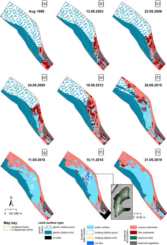
1242                     A. Kellerer-Pirklbauer et al.: Buoyant calving and ice-contact lake at Pasterze Glacier (Austria)

Table 1. Technical parameters of aerial surveys between 1998 and 2019 used in this study. For 2003, 2006, and 2009 see also Kaufmann
et al. (2015). KAGIS is the GIS Service of the Regional Government of Carinthia; BEV is the Federal Office of Metrology and Surveying.

                     Aerial survey    Acquisition date     Source                        Geometric resolution of
                                                                                          calculated orthophotos
                     1998             August 1998          Hohe Tauern National Park                      0.5 m
                     2003             13 August 2003       Kaufmann et al. (2015)                         0.5 m
                     2006             22 September 2006    Kaufmann et al. (2015)                         0.5 m
                     2009             24 August 2009       Kaufmann et al. (2015)                         0.5 m
                     2012             18 August 2012       KAGIS and BEV                                  0.2 m
                     2015             11 July 2015         KAGIS and BEV                                  0.2 m
                     2018             11 September 2018    KAGIS and BEV                                  0.2 m
                     2018             15 November 2018     AeroMap GmbH                                   0.1 m
                     2019             21 September 2019    AeroMap GmbH                                  0.09 m

IBE3 26 September 2018, IBE4 24 October 2018). The ef-               lake-level estimation was accomplished for six dates in the
fects on the proglacial landscape during these four IBEs were        period 2014–2019 (see Sect. 3.3) by identifying the lowest
quantitatively analysed as follows.                                  level of the point cloud at the lake shore (mean elevation
   For the orthorectification process of the Panomax images          of lowermost measurement points at the lake shore). Based
(7030 × 2048 px) it is necessary to find a suitable mathe-           on TLS data we observed a lake-level variation on the or-
matical model. To obtain the necessary parameters for this           der of 0.8 m and a trend in lake-level lowering during this
model, control points are needed which are visible in both           period. Therefore, as judged from our long-term as well as
the Panomax images and pre-existing orthophotos used for             short-term GNSS and TLS data, we demonstrate rather sta-
the orthorectification process. We applied an interpolation          ble lake-outflow as well as lake-level conditions at least for
approach using the rubber-sheeting model in ERDAS IMAG-              the period 2015–2020 with a lake-level lowering trend. The
INE 2018. This model calculates a triangulated irregular net-        assumption of long-term lake-level variations of < 1 m dur-
work (TIN) for all control points at the reference orthophoto        ing the summer months (seasonal amplitude) is further sup-
and at the Panomax image and transforms the calculated tri-          ported by field observations made during the last few years
angles of the oblique images in such a way that they equal           with the shape (stepped geometry) and size (< 1 m vertical
the ones of the reference orthophoto. First-degree polyno-           extent) of thermo-erosional notches at the waterline. There-
mials were used for the transformation within the triangles.         fore, the potential effect of lake-level changes on geometric
Only control points at the lake level were utilized to achieve a     errors in the orthorectified images should be small.
maximum accuracy for lake-level objects. Reasons for minor              Three groups of control points were generated using the
geometric errors in the analysed orthorectified images were          three pre-existing orthophotos of 11 July 2015, 11 Septem-
changes in the lake level or an offset of the camera (maxi-          ber 2018, and 15 November 2018 (Table 1) and suitable
mum of 5 px).                                                        Panomax images from the same days. For the IBE1 we used
   To assess the potential effect of lake-level changes on geo-      the model of 11 July 2015, for IBE2 and IBE3 the model of
metric errors in the orthorectified images, we quantified lake-      11 September 2018, and for IBE 4 the one of 15 November
level variations by using GNSS and TLS data. We compared             2018. The calculated orthorectified images have a geometric
lake-level data from nine different GNSS campaigns over              resolution of 0.2 m. ArcGIS 10.5 was subsequently used to
a 5-year period (17 September 2015–22 September 2020,                analyse landform changes.
all from the period between 11:00 and 15:00). Geometric
accuracy is in the range of centimetres based on compar-             3.5   Quantification of ice mass losses by buoyant calving
ison with stable points. Results yield a mean elevation of
2069.54 m a.s.l. ranging from 2069.87 m a.s.l. (17 Septem-           A quantification of ice losses by buoyant calving was at-
ber 2015) to 2069.19 m a.s.l. (22 September 2020) and thus           tempted by using the Panomax images. Three of the large-
a range of 0.68 m with a tendency towards lake-level low-            scale ice-breakup events occurred between August and
ering over time (Fig. 4c). In addition, we measured the el-          September 2018 (IBE2 to IBE4). For these events we esti-
evation of small and fresh-looking lake terraces next to the         mated the volume of the newly emerging icebergs and the
glacier terminus on 14 September 2020 with GNSS yielding             volume of uplifted ice masses detaching from the subaquatic
an elevation range of 0.59 m. This small elevation range is          glacier ice. The latter was accomplished by comparing the
also in accordance with the lake-level elevations measured           calculated volume of a given ice mass (e.g. a debris-covered
by GNSS during two consecutive field campaigns on 14 and             ice slab) before and after the ice-breakup event. For volu-
22 September 2020 with a difference of 0.53 m. TLS-based             metric calculations we applied the following approach. The

The Cryosphere, 15, 1237–1258, 2021                                                      https://doi.org/10.5194/tc-15-1237-2021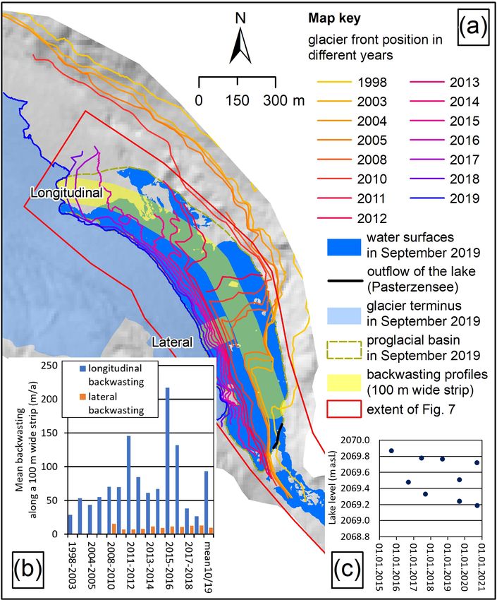
A. Kellerer-Pirklbauer et al.: Buoyant calving and ice-contact lake at Pasterze Glacier (Austria)                        1243

horizontal extent of affected (newly emerged or uplifted) ice     profile (Fig. 3b). We applied in most cases both the Wen-
masses was transferred back to and drawn into the original        ner and the Schlumberger arrays (Kneisel and Hauck, 2008).
webcam images. A maximum iceberg height was also drawn            Focus is given here on the Wenner results, which are more
as a line in the original webcam image. The length of this line   suitable for layered structures (Kneisel and Hauck, 2008).
was then quantified by using the ratio between the quantified     ERT data from 2015 and 2016 were taken from Hirschmann
horizontal extent and the marked line. The iceberg height         (2017) and Seier et al. (2017). The apparent resistivity data
was then obtained by applying a correction calculation for        were inverted in RES2DINV using the robust inversion mod-
the camera distortion produced by an incidence angle of 25◦       elling. ERT data were checked before processing for abnor-
(calculated by a height difference of 310 m and a horizontal      mally high or low resistivity values. Abnormal values are
distance of approx. 650 m).                                       commonly related to measurement errors and/or bad elec-
   The volume of individual icebergs was approximated by          trode contact usually visible at all depths. Such “bad datum
assuming that all ice bodies above the waterline have the         points” were excluded manually (Kneisel and Hauck, 2008).
form of a truncated pyramid, where A2 is 20 % (for dome-          The number of iterations was stopped when the change in the
shaped iceberg), 50 % (for mixed iceberg type), or 80 % (for      RMSE between two iterations was small.
tabular iceberg) of A1 . The volume of a truncated pyramid
(iceberg above the waterline) with an irregular base is given     3.7   Bathymetry
by
                                                                  Sonar measurements were carried out at Pasterzensee on
      h     p
                                                                  13 September 2019. Water depth in the lake was measured
V =      A1 + A1 × A2 + A2 ,                               (1)
      3                                                           with a Deeper Smart Sonar CHIRP+ system (depth range
with A1 being area at the waterline (larger base), A2 being       0.15–100 m) consisting of an echo-sounding device (single-
area of the top face (smaller base, in our cases 20 %, 50 %,      beam echo sounder) and a GNSS positioning sensor. CHIRP
or 80 % of A1 depending on iceberg type), and h being the         stands for compressed high-intensity radar pulse. We mea-
maximum height of the iceberg or truncated pyramid (Har-          sured with 290 kHz (cone angle 16◦ ) and a sonar scan rate
ris and Stöcker, 1998). With this approach we quantified the      of up to 15 s−1 . According to the producer, the 16◦ beam an-
volume of nine icebergs for IBE2 (9 August 2018), eight for       gle of the 290 kHz frequency results in a ground footprint of
IBE3 (26 September 2018), and two for IBE4 (24 October            0.28 m at 1 m water depth, of 2.81 m at 10 m water depth, and
2018). The volume above the waterline was then multiplied         of 11.24 m at 40 m water depth. These footprint values are
by 10 to calculate the total iceberg volume. Significant un-      not optimal for resolving small-scale features at large water
certainties in this quantification attempt are the visual and     depths. However, as it was intended in this study, the foot-
thus subjective estimation of the iceberg height and the fact     print values are acceptable for obtaining an overview of the
that only large icebergs are considered. Therefore, results of    lake geometry.
this approach must be seen only as orders of magnitude of            The accuracy of raw water-depth measurements depends
ice mass losses by buoyant calving in the period 9 August to      on the device used, beam angle, sonar stability, bottom com-
24 October 2018.                                                  position, and structure. Bandini et al. (2018) compared the
                                                                  Deeper Smart Sensor PRO+ system (precursor of CHIRP+)
3.6   Electrical resistivity tomography                           against the ground truth. Their results indicate a mean ab-
                                                                  solute error of 0.52 m for water depths of up to 30 m with
Electrical resistivity tomography (ERT) and seismic refrac-       almost perfect fit (ground truth vs. sonar) at shallow sites.
tion (SR) were applied in the study area between 2015 and         The tested PRO+ system underestimated the water depth at-
2019. For space reasons, we focus only on selected aspects        tributed to the beam diameter as it tends to take the shal-
of the ERT results in this paper. Electrical resistivity is a     lowest point in the beam as the depth reading when going
physical parameter related to the chemical composition of         over holes or slopes. No such comparative studies are pub-
a material and its porosity, temperature, and water and ice       lished for the CHIRP+ system. However, according to the
content (Kneisel and Hauck, 2008). For ERT a multielec-           producer the absolute error should be lower for the CHIRP+
trode and multichannel system (GeoTom 2D system, Geolog,          system (personal communication by the technical support of
Germany) and two-dimensional data inversion (RES2DINV)            Deeper, 16 December 2020). In conclusion, the estimated ac-
using finite-difference forward modelling and quasi-Newton        curacy of raw water-depth measurements should be less than
inversion techniques (Loke and Parker, 1996) was applied.         0.1 m at shallow (< 5 m) and flat sites but might be as high
ERT was carried out at a total of 43 profiles (3 in 2015, 4 in    as 0.5 m for deeper and sloping locations.
2016, 4 in 2017 – Fig. 3a and b, 5 in 2018, and 27 in 2019 –         The CHIRP+ system was mounted on a Styrofoam plat-
Fig. 3c) with 2 or 4 m electrode spacing and profile lengths of   form for stability reasons and dragged behind a small (and
80–196 m. Saltwater was sometimes used at the electrodes to       rather unstable) inflatable canoe operated by two people.
improve electrical contact. RTK GNSS was applied to mea-          Altogether 4276 water-depth measurements along a 4.3 km
sure the position of each electrode and thus the course of the    long route were accomplished (Fig. 1d). Because icebergs

https://doi.org/10.5194/tc-15-1237-2021                                               The Cryosphere, 15, 1237–1258, 2021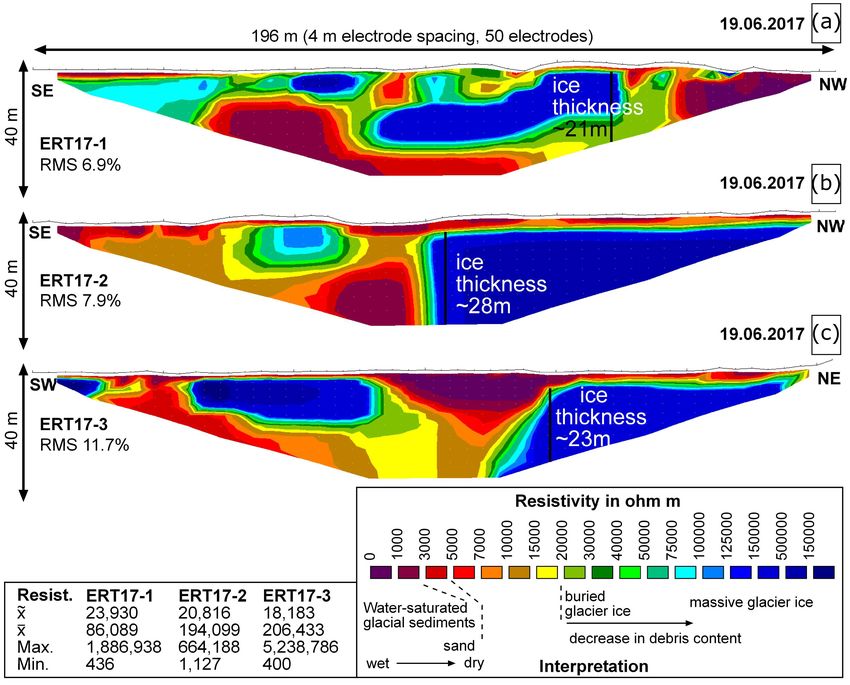
1244                       A. Kellerer-Pirklbauer et al.: Buoyant calving and ice-contact lake at Pasterze Glacier (Austria)

Figure 3. Field impressions of the ice-contact lake and its close surrounding: (a) overview image depicting the distribution of water bodies,
icebergs, and debris-covered dead-ice bodies on 19 June 2017. Courses of ERT profiles presented in Fig. 9 are shown. (b) Starting point of
ERT17-1 surveyed by GNSS. (c) Thermokarst-affected area with courses of two ERT profiles on 10 September 2019. Note Pasterze Glacier
and thermo-erosional notches at the lake level. (d) Buoyant calving of a small iceberg (“shooter”) ca. 200 m from the subaerial glacier front
observed during fieldwork (all photographs by Andreas Kellerer-Pirklbauer).

and wind cause boat instability, the canoe was not navigated             of the glacier tongue receded up-valley beyond the proglacial
along a regular shore-to-shore route but rather in a zigzag              basin. The west part of the glacier tongue is still in con-
mode starting in the northwest of the lake and ending in the             tact with the proglacial lake and changed morphologically
southeast. GNSS and water-depth data were imported into                  rather little during the last 2 decades. Figure 4a also depicts
ArcGIS for further analysis. To compute the lake geometry,               100 m wide strips where mean values for longitudinal and
the measured lake depth values and a lake mask of September              lateral backwasting were calculated. Results are shown in
2019 were combined using the Topo to Raster interpolation                Fig. 4b. The longitudinal backwasting rate was between 29.0
tool to calculate a digital terrain model (DTM) with a 5 m               and 217.2 m yr−1 , 2 to 19 times larger than the lateral back-
grid resolution. Lake volume was calculated using the func-              wasting rate of 7.3 to 13.2 m yr−1 . High annual longitudi-
tional surface toolset.                                                  nal backwasting rates were measured in most years when the
                                                                         glacier was in the basin. Since 2017, this rate has drastically
                                                                         dropped, presumably due to the detachment of the glacier
4     Results                                                            from the lake.
                                                                            Figure 5 illustrates glacier recession and the evolution of
4.1    Glacier recession and areal expansion of the lake                 proglacial water bodies for the period 1998–2019 in relation
                                                                         to the 0.365 km2 proglacial basin as defined for September
Figure 4a depicts the terminus positions between 1998 and                2019. An animation showing the general evolution of the
2019 as well as the proglacial water surfaces including                  proglacial lake between 2010 and 2020 is published in the
Pasterzensee and the proglacial basin as defined for Septem-             Supplement. In 1998 only 0.5 % of the basin was covered by
ber 2019 (area of 0.365 km2 ). The glacier steadily receded              water (Fig. 5a). Up to 2006, water surfaces still covered less
into the current proglacial basin over a longitudinal distance           than 5 % of the basin (Fig. 5c). By 2009, this value increased
of about 1.4 km. In detail, however, this recession was not              to 11.2 % (Fig. 5d) and was rather constant until 2 years later
evenly distributed along the glacier margin due to differential          (Fig. 5f). By 2016, more than 50 % of the basin was cov-
ablation below the uneven supraglacial debris. The east part

The Cryosphere, 15, 1237–1258, 2021                                                           https://doi.org/10.5194/tc-15-1237-2021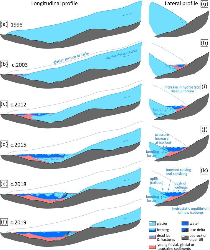
A. Kellerer-Pirklbauer et al.: Buoyant calving and ice-contact lake at Pasterze Glacier (Austria)                                   1245

                                                                         4.2   Land cover change in the lake-proximal
                                                                               surrounding since 1998

                                                                         Different glacial and proglacial surface types and landforms
                                                                         were mapped for a 0.76 km2 area in the glacial–proglacial
                                                                         transition zone for nine different stages between 1998 and
                                                                         2019 (Fig. 7). The visual landform classification gives a more
                                                                         detailed picture on landform changes in the area of interest.
                                                                         Figure 6b quantitatively summarizes the relative changes in
                                                                         different surface types in this transition zone. Debris-poor,
                                                                         rather clean ice covered 58 % of the area in 1998, decreased
                                                                         to 9.3 % until 2015, and vanished afterwards from the area.
                                                                         In contrast, debris-rich glacier parts covered in all nine stages
                                                                         between 20.5 % (2019) and 33.4 % (2015) of the transition
                                                                         zone. For this class, areal losses due to glacier recession
                                                                         were partly compensated for by areal gains due to an in-
                                                                         crease in supraglacial debris-covered areas. Water surfaces
                                                                         increased from 2.1 % in 1998 to 45.5 % in 2019. The low
                                                                         value for 15 November 2018 is related to ice floes (3.4 %),
                                                                         and data gaps (4.1 %), as well as to high values for both
                                                                         debris-rich (2.1 %) and debris-poor (1.5 %) icebergs. Areas
                                                                         covered by bedrock and vegetation were always around 4 %.
                                                                         Areas covered by fine-grained sediments reached a maxi-
                                                                         mum in 2012, decreasing substantially afterwards (mainly
                                                                         due to lake extension). Areas covered by coarse-grained sed-
Figure 4. Terminus position of Pasterze Glacier for the period 1998      iments increased from 3.3 % in 1998 to about 26 %–27 %
to 2019 and lake-level variability in Pasterzensee in the period 2015
                                                                         in 2018 and 2019 and are located at the northern and east-
to 2020 derived mainly from sequential GNSS data. (a) The extent
                                                                         ern margin of the basin. Finally, dead-ice holes were mapped
of water surfaces including Pasterzensee and the delineation of the
proglacial basin is shown for September 2019. The 100 m wide pro-        for all stages, but their spatial extent was always very small
files (lateral and longitudinal) used for backwasting calculations are   (maximum in 2012 with a total area of 618 m2 ) and covered
indicated. Backwasting results are depicted in (b) (background hill-     less than 0.1 % of the basin.
shade based on 10 m DTM, KAGIS). (c) Lake-level elevations for
nine stages between 17 September 2015–22 September 2020 (all             4.3   Buoyant calving at the ice-contact lake
between 11:00 and 15:00).
                                                                         Four large-scale ice-breakup events (IBEs) related to buoy-
                                                                         ancy were detected for the period September 2016 to October
ered by water (Fig. 5k), and in 2019 water surfaces in the               2019 (IBE1 20 September 2016, IBE2 9 August 2018, IBE3
basin covered 83.2 % (Fig. 5n). The increase in water surface            26 September 2018, and IBE4 24 October 2018). Twelve
areas in the basin since 1998 follows an exponential curve               smaller to mid-sized iceberg-tilting or capsize events were
(Fig. 6a). However, in single years this areal increase fol-             additionally documented by the Panomax images (27 May
lows a distinct pattern with enlargement of water surfaces               2017, 28 May 2017, 9 June 2017, 11 June 2017, 20 June
during summer and a decrease in autumn due to lake-level                 2017, 5 July 2017, 19 July 2017, 25 September 2017, 22 June
lowering as revealed by field observations. The exceptionally            2018, 23 September 2018, 26 September 2018, and 30 Octo-
low value of November 2018 (62.4 %) in relation to Septem-               ber 2018).
ber 2018 (73.2 %) is related to the widespread existence of                 IBE1 occurred on 20 September 2016. Figure 8a presents
ice floes. Figure 6a also depicts the extent of icebergs in the          two ortho-images from this event at its beginning (09:00) and
proglacial basin with values below 1 % in most cases. High               its end (11:15). The latter also indicates the position of the
percentage values were only mapped for 15 November 2018                  geoelectric profile ERT17-1 for orientation. Figure 2 visual-
(7.3 %) followed by rapid iceberg loss during the ablation               izes the same event. An animation depicting this ice-breakup
season in 2019.                                                          event is published in the Supplement. Different processes oc-
                                                                         curred as indicated by the capital letters in Fig. 8a: limnic
                                                                         transgression (A and F) of water due to tilting of ice slabs,
                                                                         uplift of a debris-covered ice slab (B and G), formation of
                                                                         a massive crevasse (C), complete ice disintegration (D), ice
                                                                         disintegration and lateral displacement of several ice slabs

https://doi.org/10.5194/tc-15-1237-2021                                                        The Cryosphere, 15, 1237–1258, 2021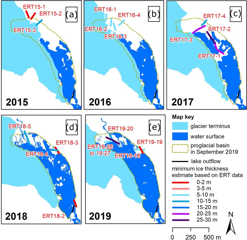
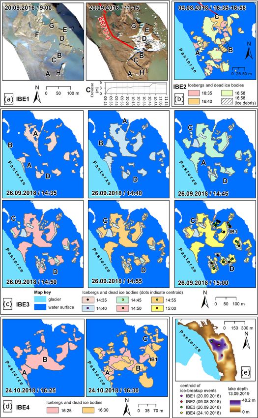
1246                      A. Kellerer-Pirklbauer et al.: Buoyant calving and ice-contact lake at Pasterze Glacier (Austria)

Figure 5. Glacier recession and evolution of proglacial water surfaces since 1998 at Pasterze Glacier. The proglacial basin as defined for
September 2019 is depicted on all maps for comparison. For data sources refer to text and Table 1. A is airborne photogrammetry; T is
terrestrial laser scanning; G is GNSS.

(E), and drying out of a meltwater channel (H). All processes          by lateral push (E) and lowering of the surface of previously
apart from the limnic transgressions ended by 11:15; the lat-          tilted slabs (B).
ter terminated at 15:30. The formation of the large crevasse               IBE2 happened on 9 August 2018. Figure 8b depicts the
started at 09:30, followed by a rapid widening until 09:45             changes that occurred between 16:35 and 16:58. At this event
(crack width 3.5 m), steady conditions until 10:45, and a sec-         three different processes were identified: (A) detachment of a
ond widening phase (crack width 5.5 m) until 10:50 (see inset          debris-covered ice peninsula (945 m2 ) from Pasterze Glacier
graph in Fig. 8a). The morphologically most distinct event             at the western lakeshore and separation into four icebergs (to-
happened between 09:50 (Fig. 2d) and 09:55 (Fig. 2e) when              tal area 1054 m2 ) and (B) emergence of a 1035 m2 large ice-
the total collapse of a 1700 m2 large ice slab occurred accom-         berg (16:35–16:40) followed by capsizing and partial disin-
panied by lateral shift and tilting of neighbouring ice slabs          tegration of this iceberg into ice debris (16:40–16:58) push-

The Cryosphere, 15, 1237–1258, 2021                                                         https://doi.org/10.5194/tc-15-1237-2021
A. Kellerer-Pirklbauer et al.: Buoyant calving and ice-contact lake at Pasterze Glacier (Austria)                                      1247

Figure 6. Glacial–proglacial transition zone: (a) evolution of water surfaces and icebergs in the proglacial basin (100 % = 0.37 km2 ; Fig. 5
for delineation) of Pasterze Glacier since 1998 based on airborne photogrammetry (A) or terrestrial laser-scanning (T) data. Icebergs only
based on airborne photogrammetry (A). (b) Summarizing graph depicting relative changes in different surface types in the glacial–proglacial
zone (100 % = 0.76 km2 ; extent as shown in Fig. 7) since 1998.

ing away other icebergs which causes (C) lateral iceberg dis-            (12.9 m draft, 1.4 m freeboard). Therefore, in order to have
placement of up to 65.6 m as well as a clockwise iceberg ro-             a freely moveable iceberg, a water depth exceeding 13 m is
tation of 95◦ .                                                          needed.
   IBE3 occurred on 26 September 2018. This event involved                  No large buoyant calving events were detectable in the
four main processes as visualized in Fig. 8c: (A) uplift of              time-lapse images after 24 October 2018. However, at least
debris-covered ice bodies increasing the surface area from               the occurrence of small-sized buoyant calving events which
6820 to 13 245 m2 in only 10 min (at 14:35–14:45), (B) emer-             are hardly detectable by the time-lapse camera can be as-
gence of a new iceberg between 14:35 and 14:40 which cap-                sumed. During fieldwork in June 2019, we observed buoyant
sized a few minutes afterwards, (C) limnic transgression, and            calving of a small, ca. 3 m long iceberg (“shooter” accord-
(D) lateral iceberg displacement (both C and D at 14:35–                 ing to Benn and Evans, 2010) ca. 200 m from the subaerial
15:00). At the southern part of the affected area, icebergs              glacier front (Fig. 3d). The whole event took only few min-
moved away from the uplifting area (push effect). In con-                utes and was hardly visible in the time-lapse images of that
trast, at the eastern part of the affected area icebergs moved           particular day.
towards the uplifting area possibly due to compensatory cur-
rents causing a suction effect. A large iceberg (IB1 in Fig. 7c)         4.4   Ice mass loss by buoyant calving and subaerial
was hardly moving at all suggesting grounding conditions.                      ablation
   The last major IBE took place on 24 October 2018 (IBE4)
spanning only 5 min (Fig. 8d). Like IBE2, a debris-covered               The quantification of the ice loss by buoyant calving for the
ice peninsula (1933 m2 ) detached from Pasterze Glacier at               three events IB2 to IB4 approximated by ice detachment, up-
the western lakeshore and separated into several icebergs                lift, and emergence processes revealed the following results.
(A). Furthermore, (B) ice disintegration and (C) lateral ice-            The sums of movement-affected ice masses (without lat-
berg displacement were observed during the event. The large              eral displacement) during the three ice-breakup events were
iceberg IB1 experienced a lateral offset of 22 m accompa-                55 717 m3 for IBE2, 445 257 m3 for IBE3, and 537 604 m3
nied by a clockwise rotation by 43◦ . The spatial extent, vol-           for IBE4, summing up to 1 038 578 m3 (Table 2). As no other
ume, and freeboard of this iceberg were calculated based on              substantial ice-breakup events occurred afterwards, we can
a high-resolution DTM derived from the aerial survey dating              therefore assume that ice loss by buoyant calving in the pe-
to 15 November 2018 (see Table 1). The subaerial volume                  riod August 2018 to August 2019 at Pasterze Glacier was at
of iceberg IB1 was 3271 m3 on 15 November 2018, which                    least on the order of 1 × 10⁶ m3 .
should be around 10 % of the entire iceberg. Hence, approx-                 The comparison of the two sets of TLS data from
imately 29 500 m3 (90 %) was below the lake level during                 13 September 2018 and 3 August 2019 revealed surface el-
that time. Maximum freeboard of IB1 was 3.7 m with a mean                evation changes and thus more or less glacier ice ablation
freeboard value of 1.4 m. If we assume the same surface area             of up to 5 m between the two stages. It was not within the
of the iceberg below the lake level (2287 m2 ), we could fur-            scope of this paper to analyse ablation rates at the terminus
ther assume a mean ice thickness of the iceberg of 14.3 m                of Pasterze Glacier in detail. However, for a rough estimate

https://doi.org/10.5194/tc-15-1237-2021                                                         The Cryosphere, 15, 1237–1258, 2021
1248                      A. Kellerer-Pirklbauer et al.: Buoyant calving and ice-contact lake at Pasterze Glacier (Austria)

Figure 7. Land cover evolution in the glacial–proglacial transition zone (0.76 km2 ) of Pasterze Glacier between 1998 and 2019 based on
visual landform classification. The proglacial basin as defined for September 2019 is depicted in all maps for comparison. For data sources
refer to text and Table 1. Inset map in (h) depicts a digital elevation model and contour lines (0.5 m interval) of iceberg IB1.

we can calculate for the lowest part of the glacier tongue next         4.5   Ground ice conditions at the lake basin and its
to the proglacial lake (see Fig. 1, ca. 0.35 km2 ) the total ice              proximity
loss for the period September 2018 to August 2019. Mean ab-
lation rates of 2.5 or 3.0 m for this area would yield total ice        Altogether 43 ERT profiles were measured in the proglacial
losses by ablation for this area of 870 000 and 1 050 000 m3 ,          area between 2015 and 2019 with profile lengths of be-
respectively.                                                           tween 80 and 196 m. In this study we focus on the quan-

The Cryosphere, 15, 1237–1258, 2021                                                          https://doi.org/10.5194/tc-15-1237-2021
A. Kellerer-Pirklbauer et al.: Buoyant calving and ice-contact lake at Pasterze Glacier (Austria)                                  1249

Figure 8. Ice-breakup events (IBEs) at the ice-contact lake Pasterzensee monitored by time-lapse photography: (a) IBE1 20 September 2016;
(b) IBE2 9 August 2018; (c) IBE3 26 September 2018; (d) IBE 4 24 October 2018; (e) overview map of the events. Capital letters on the
maps indicate different processes (for details see text).

https://doi.org/10.5194/tc-15-1237-2021                                                      The Cryosphere, 15, 1237–1258, 2021
1250                        A. Kellerer-Pirklbauer et al.: Buoyant calving and ice-contact lake at Pasterze Glacier (Austria)

Table 2. Affected ice masses during the three ice-breakup events IBE2 (9 August 2018), IBE3 (26 September 2018), and IBE4 (24 October
2018). For approach see text. Numbers in bold are not considered for the total volume calculation. Lateral displacement of icebergs is not
considered.

                     Event       Process                    State                Volume above water     Total volume
                                                                                   level – 10 % (m3 )   – 100 % (m3 )
                     IBE2        ice peninsula detachment   before detachment                 3206.8          32 068
                                 ice emergence              after emergence                   2364.8          23 648
                     IBE3        ice emergence              after emergence                  3216.9           32 169
                                 ice uplift                 before uplift                    7060.3           70 603
                                                            after uplift                    48 369.2         483 692
                                                            difference                      41 308.9        413 089∗
                     IBE4        ice peninsula detachment   before detachment                2833.6           28 336
                                 ice disintegration         after emergence                 50 926.8         509 268
                     Sum                                                                                   1 038 578
                   ∗ Difference considered in the total.

tification of sediment-buried dead-ice bodies detected by               or only very small occurrences of glacier ice (ERT19-19,
ERT. A detailed discussion on the ERT results will be pre-              1 m ice). The three profiles near the northwestern shore of
sented elsewhere. Resistivity values of > 20 000 m indi-               the lake revealed minimum ice thickness estimates of up
cate buried glacier ice, and water-saturated glacial sediments          to 26 m (ERT19-26). In summary, ERT profiles outside the
show values of < 3000 m (Pant and Reynolds, 2000). Clay                proglacial basin typically showed few buried dead-ice rem-
and sand have resistivity values in the ranges of 1–100 and             nants, whereas profiles in the basin (particularly at its north-
100–5000 m, respectively. Temperate glacier ice may ex-                western part) typically yielded resistivity values consistent
ceed 1 × 10⁶ m (Kneisel and Hauck, 2008). We used the                  with widespread massive dead ice.
20 000 m-boundary in the interpretation to estimate the
maximum ice thickness for each profile as depicted in Fig. 9            4.6     Bathymetry of the lake basin
which shows three profiles from 2017. In many cases, ice
thickness exceeded the depth of ERT penetration. Therefore,             Lake-bottom geometry and the water volume of Pasterzensee
we were only able to calculate “minimum ice thickness esti-             were calculated based on 4276 sonar measurements (Fig. 1d).
mates” based on the ERT data.                                           Measured water depths ranged from 0.35 to 48.2 m yield-
    Figure 10 summarizes the results of the surveys for 2015,           ing an arithmetic mean of 13.4 m and a median of 10.7 m.
2016, 2017, 2018, and September 2019. Two of the three                  During the time of bathymetric measurements, the lake level
ERT profiles measured in 2015 (ERT15-1, ERT15-2) re-                    was 2069.1 m a.s.l. implying that the lowest point at the
vealed only very thin ice lenses. Both are located outside              lake bottom was 2020.9 m a.s.l. (Fig. 11). Several sub-basins
the proglacial basin as defined in September 2019 (Fig. 10a).           (marked as A–D in Fig. 11a) were identified along the 1.2 km
The profile in the basin had an estimated ice thickness of              long and up to 300 m wide lake basin. One small sub-basin
14 m (ERT15-3). The profiles measured in 2016 revealed                  (A) was detected close to the southern end of the lake with
minimum ice thickness values of 8–10 m (Fig. 10b). The                  maximum measured water depths exceeding 20 m (maxi-
four profiles measured in 2017 in the central part of the               mum 24.1 m, 2045 m a.s.l.), an E–W extent of 160 m, and a
proglacial area revealed minimum ice thicknesses of between             N–S dimension of 140 m. A second sub-basin (B) is slightly
13 (ERT17-4) and 28 m (ERT17-2) (Fig. 10c) confirming the               less deep (max 20.5 m) but seems to be broader compared to
existence of massive dead ice beneath a thin veneer of debris           basin (A). The third sub-basin (C) is by far the deepest, the
(Fig. 9).                                                               largest, and the most complex one with a maximum water
    The interpretations of four profiles measured in 2018 are           depth of 48.2 m and a secondary basin in the south reaching
shown in Fig. 10d. Profiles ERT18-2 and ERT18-3 are free                a measured maximum depth of 31.0 m. In this sub-basin, wa-
of ice located outside the basin or at its margin. ERT18-4 and          ter depths exceeding 30 m were calculated for a 34 000 m2
ERT18-5 were both located in the basin and revealed mini-               large area in the central part of the entire lake basin. The lake
mum ice thicknesses of 13 (ERT18-5) and 14 m (ERT18-4).                 basin becomes generally shallower towards the northwest.
The September-2019 measurements supported earlier mea-                  Finally, a fourth sub-basin (D) was identified at the north-
surements (Fig. 10e). The profiles at the eastern margin of             western end of Pasterzensee where a broad basin is located
the basin showed again a thin layer (ERT19-18, 8 m ice)                 with a maximum measured depth of 17.7 m. Based on our
                                                                        gridded DTM for the lake bottom, the estimated water vol-

The Cryosphere, 15, 1237–1258, 2021                                                          https://doi.org/10.5194/tc-15-1237-2021
A. Kellerer-Pirklbauer et al.: Buoyant calving and ice-contact lake at Pasterze Glacier (Austria) 1251
Figure 9. ERT results (Wenner array) and interpretation of three profiles (50 electrodes, 4 m spacing, length 196 m) measured in the proglacial
area of Pasterze Glacier on 19 June 2017 (location: Figs. 3 and 10). Summary statistics in the inset table: (a) ERT17-1 – ice lens with a
thickness of ca. 21 m, (b) ERT17-2 – ice thickness ca. 28 m, and (c) ERT17-3 – ice thickness ca. 23 m. For (b) and (c) – ice thickness
exceeded the depth of ERT penetration.
ume of the 299 496 m2 large lake Pasterzensee in September tongue caused by an uneven distribution of the supraglacial
2019 was 4×10⁶ m3 . The gradient from the deep basin (C) to debris cover (Kellerer-Pirklbauer, 2008). The debris cover
the shore seems to be rather gradual at the eastern margin of distribution pattern promotes differential ablation (Kellerer-
the lake. In contrast, at the western margin of the lake basin Pirklbauer et al., 2008). Rapid deglaciation as well as glacier
where Pasterzensee is in ice contact, the gradient is steep in thinning is much more intensive at the debris-poor part of
most areas (e.g. at sub-basin C – horizontal distance between the glacier affecting the stress and strain field and modifying
sonar measurement location and glacier margin 19 m vs. wa- the flow directions of the ice mass (Kaufmann et al., 2015).
ter depth 26.1 m) suggesting a steep glacier margin with a Therefore, the proglacial lake predominantly developed in ar-
pronounced ice foot. eas where debris-poor ice was located before.
At the waterline, thermo-erosional undercutting causes the
formation of notches (cf. Röhl, 2006). Such notches are fre-
5 Discussion quent features at Pasterze Glacier and were first reported
in 2004 (Kellerer-Pirklbauer, 2008). GNSS measurements
5.1 Glacial-to-proglacial landscape modification at the glacier margin on 13 September 2019 showed that
waterline notches occurred during that time at 53 % of the
Pasterze Glacier receded by some 1.4 km between 1998 935 m long ice-contact line between Pasterze Glacier and
and 2019 thereby causing the formation of a bedrock- Pasterzensee (Fig. 5n). Notches observed at Pasterze Glacier
dammed lake in an over-deepened glacial basin. During during several September field campaigns during the last few
these 2 decades, the glacier decelerated, fractured (Kellerer- years had a stepped geometry due to lake-level drop. The am-
Pirklbauer and Kulmer, 2019), and lost the connection to plitude of water-level fluctuations at Pasterzensee in the pe-
the lake at its eastern part. In contrast, at the western shore, riod 2015 to 2020 was less than a metre based on GNSS and
the lake was still in ice contact with the glacier in 2019. TLS data, indicating rather stable lake-outflow conditions.
This ice-contact difference is related to an unequal reces-
sion pattern of the eastern and western part of the glacier
https://doi.org/10.5194/tc-15-1237-2021 The Cryosphere, 15, 1237–1258, 20211252 A. Kellerer-Pirklbauer et al.: Buoyant calving and ice-contact lake at Pasterze Glacier (Austria)
Figure 10. Interpreted minimum ice thicknesses based on electri-
cal resistivity tomography (ERT) data (for estimation approach see
Fig. 9) in the proglacial area of Pasterze Glacier for (a) 30 Septem-
ber 2015, (b) 13 September 2016, (c) 19 June 2017, (d) 13 Septem-
ber 2018, and (e) 9 September 2019 as well as 10 September 2019.
“Minimum” means in this case that the base of the ice core was
commonly below the depth of ERT penetration.
Figure 11. Lake bathymetry based on echo-sounding data acquired
However, GNSS and TLS data both show a lake-level lower- in 2019 and its relationship to the ERT data from 2017: glacier ex-
tent and lake bathymetry in September 2019 (5 m grid resolution);
ing trend since 2015.
the extent of the proglacial basin as defined for September 2019 is
Stepped geometries have also been observed at other drawn on the map for orientation.
alpine lakes (e.g. Röhl 2006). Rates of notch formation and,
thus, of thermo-erosional undercutting at Pasterze Glacier
are unknown. However, if we consider the annual lateral by 2016, and 83 % by 2019. On an annual timescale water
backwasting rates derived from GNSS data (Fig. 4) indica- surface changes follow a distinct pattern with enlargement
tive of thermo-erosional undercutting, a mean melt rate of during summer due to glacier and dead-ice ablation in lake-
about 10 m yr−1 for the period 2010–2019 can be assumed. contact locations, causing lake transgression and a shrinkage
This is about one-third of the values quantified for Tasman in size in autumn due to lake-level lowering. This annual pat-
Glacier (Röhl, 2006). The difference is possibly related to tern at Pasterzensee has also been detected and quantified by
cooler (higher-elevation) and more shaded (NE-facing) con- Sentinel-1 and Sentinel-2 data (Avian et al., 2020).
ditions at Pasterze Glacier. Outward toppling of undercut ice Carrivick and Tweed (2013) discuss the enhanced ablation
masses due to thermal erosion, a process potentially rele- at ice-contact lakes via mechanical and thermal stresses at the
vant for calving at ice-contact lakes (Benn and Evans, 2010), glacier–water interfaces. They report increasing lake sizes in
was not observed at Pasterze Glacier. Lateral backwasting the proglacial area of Tasersuaq Glacier, west Greenland, for
at Pasterze Glacier is mainly controlled by ice melting either four different stages between 1992 and 2010. An exponen-
beneath supraglacial debris or at bare ice cliffs above notches tial increase in lake size, as observed at Pasterze Glacier, was
where the slope is too steep to sustain debris cover, and thus however not observed at Tasersuaq Glacier as judged from
the rock material slides into the lake (see Fig. 10 in Kellerer- their provided map in the paper. More general, detailed stud-
Pirklbauer, 2008). ies of increasing lake size on an annual basis are rare, imped-
The analysis of the relationship between glacier reces- ing the comparison of our results with other studies accom-
sion and the evolution of proglacial water surfaces showed plished in similar topoclimatical settings. Some comparative
drastic changes in 1998–2019. The spatial extent of water observations are, however, as follows.
surfaces in the 0.37 km2 proglacial basin followed an ex-
ponential curve with 0.5 % in 1998, 21 % by 2013, 51 %
The Cryosphere, 15, 1237–1258, 2021 https://doi.org/10.5194/tc-15-1237-2021You can also read