A global model perturbed parameter ensemble study of secondary organic aerosol formation - Recent
←
→
Page content transcription
If your browser does not render page correctly, please read the page content below
Atmos. Chem. Phys., 21, 2693–2723, 2021
https://doi.org/10.5194/acp-21-2693-2021
© Author(s) 2021. This work is distributed under
the Creative Commons Attribution 4.0 License.

A global model perturbed parameter ensemble study
of secondary organic aerosol formation
Kamalika Sengupta1 , Kirsty Pringle1 , Jill S. Johnson1 , Carly Reddington1 , Jo Browse2 , Catherine E. Scott1 , and
Ken Carslaw1
1 Institute  for Climate and Atmospheric Science, School of Earth and Environment, University of Leeds, Leeds, UK
2 Centre   for Geography and Environmental Science, University of Exeter, Penryn, Cornwall, UK

Correspondence: Kamalika Sengupta (k.sengupta@leeds.ac.uk)

Received: 22 July 2020 – Discussion started: 12 August 2020
Revised: 7 December 2020 – Accepted: 7 December 2020 – Published: 23 February 2021

Abstract. A global model perturbed parameter ensemble of           1   Introduction
60 simulations was used to explore how combinations of
six parameters related to secondary organic aerosol (SOA)
formation affect particle number concentrations and organic        About 20 %–50 % of lower-tropospheric fine aerosol mass in
aerosol mass. The parameters represent the formation of or-        continental mid-latitudes and almost 90 % in the tropics is
ganic compounds with different volatilities from biogenic          composed of organic material (Kanakidou et al., 2005). The
and anthropogenic sources. The most plausible parameter            major fraction of organic aerosol has been found to be sec-
combinations were determined by comparing the simulations          ondary (Zhang et al., 2007; Jimenez et al., 2009), formed as
against observations of the number concentration of parti-         a result of atmospheric oxidation of volatile organic com-
cles larger than 3 nm diameter (N3), the number concentra-         pounds (VOCs) leading to secondary organic aerosol (SOA).
tion of particles larger than 50 nm diameter (N50), and the        Estimating atmospheric SOA is important for accurately es-
organic aerosol (OA) mass concentration. The simulations           timating the anthropogenic aerosol radiative forcing (Maria
expose a high degree of model equifinality in which the skill      et al., 2004; Tsigaridis and Kanakidou, 2007; Carslaw et al.,
of widely different parameter combinations cannot be dis-          2010; Riipinen et al., 2011; Makkonen et al., 2012; Shri-
tinguished against observations. We therefore conclude that,       vastava et al., 2017; Tsigaridis and Kanakidou, 2018). De-
based on the observations we have used, a six-parameter            spite the importance of SOA for climate, a comprehensive
SOA scheme is under-determined. Nevertheless, the model            characterization of atmospheric VOCs, their reaction path-
skill in simulating N3 and N50 is clearly determined by the        ways, and their SOA formation potential has not yet been
low-volatility and extremely low-volatility compounds that         possible. Characterization of VOCs is challenging because
affect new particle formation and growth, and the skill in         of the very large number of compounds involved and their
simulating OA mass is determined by the low-volatility and         diverse sources; tens of thousands of VOCs have been iden-
semi-volatile compounds. The biogenic low-volatility class         tified in the atmosphere and yet more still remain to be de-
of compounds that grow nucleated clusters and condense on          tected (Goldstein and Galbally, 2007). For the SOA precur-
all particles is found to have the strongest effect on the model   sor gases that have been identified, questions remain about
skill in simulating N3, N50, and OA. The simulations also          their emission sources, their chemical conversion to SOA,
expose potential structural deficiencies in the model: we find     and the effects of atmospheric chemical composition and ox-
that parameter combinations that are best for N3 and N50           idants on SOA formation.
are worst for OA mass, and the ensemble exaggerates the                From a modelling perspective a further challenge is how
observed seasonal cycle of particle concentrations – a defi-       to deal with the enormous chemical complexity of the sys-
ciency that we conclude requires an additional anthropogenic       tem to adequately parameterize laboratory and observational
source of either primary or secondary particles.                   results and incorporate them in large-scale models. Models
                                                                   traditionally use laboratory measurements of reaction rate

Published by Copernicus Publications on behalf of the European Geosciences Union.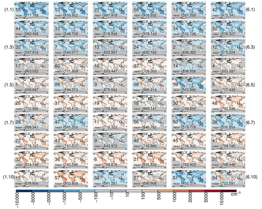
2694                                                  K. Sengupta et al.: A global model perturbed parameter ensemble study

constants and product yields to calculate the production of           tween a nine-species VBS approach and a simplified two-
highly oxidized VOCs from the reaction between precursor              species VBS approach, the latter being a factor of 2 lower in
VOCs and atmospheric oxidants. Only a very small range                computational cost. Shrivastava et al. (2011) concluded the
of natural VOCs are accounted for, such as monoterpenes               two-species approach is well-suited to represent the complex
or isoprene. Uptake of SOA onto particles is then simulated           evolution of atmospheric organic aerosols. Riipinen et al.
either time-dependently (often called kinetic uptake) or as-          (2011) and Scott et al. (2015) propose a simplified SOA for-
suming thermodynamic partitioning (Riipinen et al., 2012).            mation scheme representing species of two volatilities. Tsi-
Such “bottom-up” approaches to simulating SOA predict a               garidis et al. (2014) show global model skill does not increase
global SOA budget at the lower end of the total uncertainty           with model complexity with regard to organic aerosol mass
range (Kanakidou et al., 2005), most likely because simu-             concentrations.
lations do not capture the full range of VOCs and atmo-                  There is the risk that added complexities in models that
spheric oxidative pathways that lead to a range of products           are not well-constrained by experimental data could increase
of varying volatilities (Hallquist et al., 2009; Tsigaridis et al.,   model uncertainty and thereby introduce more uncertainty
2014). Studies like Heald et al. (2005), Johnson et al. (2006),       in the quantification of the effect of anthropogenic aerosols
and Spracklen et al. (2011) show that models have consis-             (Lee et al., 2016). Although model complexity is increased
tently and significantly underestimated SOA concentrations            in order to improve the representation of the physical, chem-
in different parts of the atmosphere. Tsigaridis et al. (2014)        ical, or optical properties of SOA (Tsigaridis et al., 2014), a
show models largely underestimate the amount of organic               more complex model that matches some observations may
aerosol present in the atmosphere with the underestimation            not have lower uncertainty in making predictions because
being strongest in urban regions based on a study involving           of the increased likelihood of compensating errors, often
31 global models.                                                     called model equifinality (Beven, 2006). The simulated par-
   It is well-established that atmospheric organic molecules          ticle number (and anthropogenic aerosol forcing) is affected
strongly affect the number concentrations of climate-relevant         by several model parameters and their associated uncertain-
sized particles by condensing on and growing aerosol parti-           ties, some of which may be compensating for each other.
cles (Riipinen et al., 2011) or by promoting particle forma-          Tuning any one parameter within the model (e.g. the nu-
tion (O’Dowd et al., 2002; Zhang et al., 2004; Metzger et al.,        cleation rate) to improve the model performance against ob-
2010). Recent studies (Ehn et al., 2014; Jokinen et al., 2015;        servations of one aspect of the atmospheric aerosol distribu-
Kirkby et al., 2016; Tröstl et al., 2016; Bianchi et al., 2019)       tion (e.g. the total particle number concentration) may ad-
have established the importance of atmospheric highly oxy-            versely affect the model performance in other outputs (e.g.
genated organic molecules in the formation and growth of              total aerosol mass). Such tuned observationally constrained
new aerosol particles. Subsequent model simulations based             models give the impression of low aerosol uncertainty and
on these experimental data have shown that new particle               model robustness but still predict a large range of aerosol
formation involving organic molecules could explain the               forcing in Lee et al. (2016).
seasonal cycle of particle concentrations (Riccobono et al.,             In this paper we use a perturbed parameter ensemble of 60
2014) and provide a source of aerosol in clean pre-industrial         simulations of a global aerosol model to examine the effect
environments that is important for climate (Gordon et al.,            of six uncertain parameters in SOA formation on simulated
2016). It has been estimated that global cloud condensation           organic aerosol mass and particle number concentrations. We
nuclei (at 0.2 % supersaturation) would be about one-quarter          compare three model outputs against observations: the num-
lower without biogenic VOCs, and about three-quarters of              ber concentration of particles larger than 3 nm dry diameter
this effect is caused by the role of organic molecules in nu-         (N3) and 50 nm dry diameter (N50) and the mass concentra-
cleation and early growth (Gordon et al., 2017).                      tion of organic aerosol (OA). Our primary aim is to under-
   The importance of SOA for climate means that large-scale           stand the sensitivity of N3, N50, and OA to the combinations
models need to simulate the contributions of these highly             of model input parameters that control the formation of SOA.
oxygenated molecules in nucleation or subsequent particle             We identify parts of parameter space that result in the best
growth. Several modelling studies (such as Farina et al.,             agreement with observations of N3, N50, and OA. Further,
2010; Pye and Seinfeld, 2010; Jathar et al., 2011) have im-           we identify parameter combinations that produce models that
plemented the volatility basis set (VBS) framework proposed           are indistinguishable in terms of their simulations of number
by Donahue et al. (2012) for the description of organic parti-        and mass concentrations.
tioning and chemical ageing. Other SOA modelling frame-
works have been proposed by Odum et al. (1996), Cam-
redon et al. (2007), and Parikh et al. (2011). However in-
creased model complexity inevitably requires more compu-
tational resources and more runtime, both of which need
to be considered carefully by modellers. Shrivastava et al.
(2011) found comparable predictions of observed OA be-

Atmos. Chem. Phys., 21, 2693–2723, 2021                                                https://doi.org/10.5194/acp-21-2693-2021
K. Sengupta et al.: A global model perturbed parameter ensemble study                                                        2695

2     Methods                                                      sors, oxidants, and role of each ox-VOC in SOA formation
                                                                   are defined in Table 1. The ox-VOCs in this new scheme
2.1    GLOMAP global aerosol model                                 of SOA formation produced from bimolecular oxidation re-
                                                                   actions of VOCs are B_ELVOC, B_LVOC, B_SVOC_M,
We use the GLOMAP (Global Model of Aerosol Processes)              B_SVOC_I, A_LVOC, and A_SVOC. The six perturbed pa-
modal aerosol microphysics model (Mann et al., 2010),              rameters in this study are scaling factors or reaction yields
which is an extension to the TOMCAT 3-D chemical trans-            that control the concentrations of these six ox-VOCs.
port model (Chipperfield, 2006). The model has a hori-
zontal resolution of 2.8◦ × 2.8◦ , with 31 hybrid σ -pressure      2.3   Microphysical processes
levels from the surface to 10 hPa. Large-scale atmospheric
transport in the model for 2008 is driven by ERA-Interim           SOA formation in the model starts with B_ELVOC and sulfu-
reanalysis produced by the European Centre for Medium-             ric acid via nucleation. Nucleation rates in the model (Kirkby
Range Weather Forecasts (ECMWF) at 6-hourly intervals.             et al., 2016; Gordon et al., 2016) determine the formation of
The aerosol distribution is simulated using four hydrophilic       clusters of 1.7 nm dry diameter. Thereafter their growth up to
modes (nucleation, Aitken, accumulation, and coarse) and           3 nm sizes in the model is determined using the equation of
one non-hydrophilic Aitken mode. The aerosol phase has             Kerminen and Kulmala (2002), which takes into account the
four components: sulfate, sea salt, black carbon, and organic      losses during initial growth of clusters. Clusters that reach
carbon. Where more than one species is contained in a mode,        a dry diameter of 3 nm are added to the nucleation mode as
we assume internal mixing (Mann et al., 2010).                     freshly nucleated particles. Thus N3, the number concentra-
                                                                   tion of particles with dry diameter greater than 3 nm (in recip-
2.2    SOA scheme                                                  rocal cubic centimetres), represents the total particle number
                                                                   concentration in the model.
The model described in Mann et al. (2010) includes one                Once particles appear in the nucleation mode they may
SOA species produced from oxidation of monoterpenes                either grow using sulfuric acid and ox-VOCs (as described
only. In this study we produce six SOA species from oxy-           above) or get scavenged by larger particles acting as a con-
genated organic compounds derived from the oxidation of            densation sink. Particles that reach a dry diameter of 50 nm
monoterpene, isoprene, and anthropogenic sources. Monthly          can act as cloud condensation nuclei in the atmosphere. Thus
monoterpene and isoprene emissions used in the model               N50, the number concentration of particles with a dry diam-
are generated from the Community Land Model by Sarah               eter greater than 50 nm (in cm−3 ), represents the number of
Monks (MEGANv2.1; Guenther et al., 2012) Emission of               climate-relevant sized particles in the model.
anthropogenic VOC is parameterized using the approach                 Aerosol particles are removed through dry deposition, sed-
in Spracklen et al. (2011) – we use CO emissions from              imentation, nucleation scavenging, and impact scavenging.
the MACCity inventory and assume a SOA/OC mass ra-                 Dry deposition accounts for gravitational settling, Brown-
tio of 1.4. Atmospheric oxidants (OH q, O3 , NO3 q) are taken      ian motion, impaction interception, and particle rebound and
from 6-hourly monthly mean values calculated offline from a        predominantly removes particles smaller than 50 nm. Pro-
TOMCAT simulation and interpolated to the model chemical           cesses represented under wet deposition are nucleation scav-
time step (Monks et al., 2017).                                    enging and impact scavenging.
   Figure 1 shows a schematic of the treatment of SOA in this
study. Gas-phase oxygenated organic compounds (ox-VOCs)            2.4   Perturbed parameter ensemble
are represented by three classes: extremely low-volatility
(ELVOC), low-volatility (LVOC), and semi-volatile (SVOC)           Simultaneous perturbation of six model parameters within
organic compounds.                                                 each of their chosen ranges forms a 6-D parameter space
   The ELVOCs are assumed to derive only from biogenic             within which we explored the competing and compensating
sources and nucleate to form new particles that either grow or     effects of these parameters on model outputs. An ensemble
are lost to pre-existing larger particles (Gordon et al., 2016).   of 60 simulations was produced, each with a different com-
The LVOCs are assumed to condense kinetically and irre-            bination of the six parameters. Simulations were run for the
versibly (i.e. with zero vapour pressure) on all particles, and    year 2008. To ensure good coverage of the 6-D parameter un-
the SVOCs are assumed to partition into all particles, ex-         certainty space, the maximin Latin hypercube sampling tech-
cept those in the nucleation mode, in proportion to the pre-       nique (McKay et al., 1979) was used to choose the combina-
existing organic mass in the mode (Scott et al., 2015). The        tions of parameters. The Latin hypercube sampling method
LVOCs and SVOCs are further divided into biogenic (pre-            samples the entire 6-D parameter space and creates a space-
fix B) and anthropogenic (prefix A). The biogenic precursors       filling design of 60 combinations of parameter values such
are split into monoterpenes (suffix M) and isoprene (suffix        that the distance between any two points in the 6-D space is
I), with the monoterpenes allowed to form both LVOCs and           maximized. The effectivity of the Latin hypercube sampling
SVOCs and the isoprene forming only SVOCs. The precur-             method to create space-filling parameter combinations has

https://doi.org/10.5194/acp-21-2693-2021                                            Atmos. Chem. Phys., 21, 2693–2723, 2021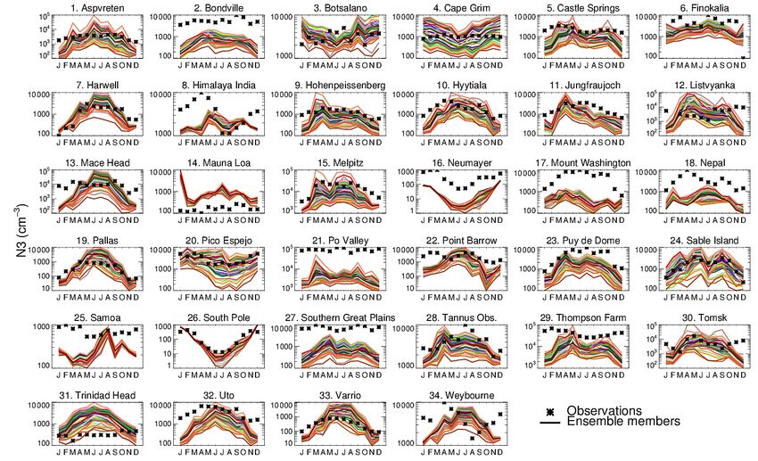
2696 K. Sengupta et al.: A global model perturbed parameter ensemble study
Figure 1. Schematic showing the SOA formation scheme in GLOMAP-mode and the six oxidized VOCs (products of photochemical ox-
idation of emitted VOCs that eventually produce SOA) whose concentrations are perturbed in this study. The six oxidized VOCs repre-
sent three volatility categories – extremely low-volatility organic compounds (ELVOCs, blue), low-volatility organic compounds (LVOCs,
green), and semi-volatile organic compounds (SVOCs, red). Prefix “A” indicates precursor gases of anthropogenic origin and “B” indi-
cates biogenic origin. The schematic shows the precursor gases and oxidants that react to produce these ox-VOCs, their relative volatility
(ELVOC < LVOC < SVOC), and the mechanism (nucleation for ELVOCs, kinetic condensation for LVOCs, and mass-based partitioning for
SVOCs) by which they add to the condensed phase (represented here by the five modes: nucleation soluble, Aitken soluble, accumulation
soluble, coarse soluble, and Aitken insoluble modes).
Table 1. List of oxidized VOCs implemented in this study, the volatility class they represent, whether produced from biogenic or anthro-
pogenic sources, how they take part in atmospheric SOA formation, parent VOC, and oxidants that react to produce each ox-VOC. MT stands
for monoterpene, IP stands for isoprene, and CO stands for carbon monoxide indicating anthropogenically sourced VOC.
ox-VOC Volatility Nature of source Role Parent VOC Oxidants
B_ELVOC Extremely low biogenic nucleation α-pinene O3 , OH q
B_LVOC Low biogenic kinetic condensation α-pinene O3 , OH q , NO3 q
B_SVOC_M Semi-volatile biogenic mass-based partition α-pinene O3 , OH q , NO3 q
B_SVOC_I Semi-volatile biogenic mass-based partition isoprene O3 , OH q , NO3 q
A_LVOC Low anthropogenic kinetic condensation anthropogenic VOCs OH q
A_SVOC Semi-volatile anthropogenic mass-based partition anthropogenic VOCs OH q
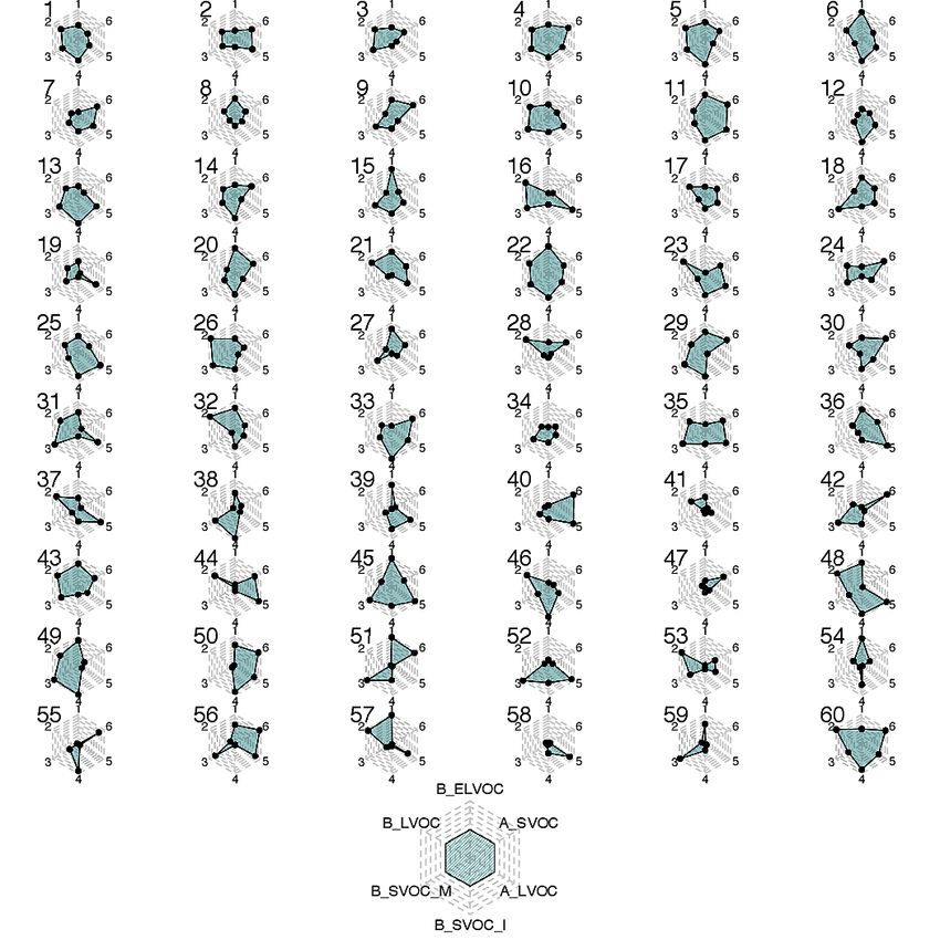
been discussed in Lee et al. (2011, 2013). The relative varia- 5 times the baseline for anthropogenic ox-VOCs (A_LVOC
tion in the ox-VOCs in each simulation is shown in Fig. 2. and A_SVOC). We perturb the concentrations of ox-VOCs
We perturb the concentrations of SOA-producing ox- taking part in the model nucleation scheme, B_ELVOC, us-
VOCs by perturbing the yields of bimolecular oxidation re- ing a scaling factor between 0 and 10, where 0 is equiva-
actions for B_LVOC, B_SVOC_M, B_SVOC_I, A_LVOC, lent to sulfuric-acid-only nucleation and 10 is equivalent to
and A_SVOC. The baseline molar yields for each of these ELVOC concentrations about a factor of 10 higher than re-
ox-VOCs before perturbation were 13 % for B_LVOC, 13 % ported in Kirkby et al. (2016). The ranges (Table 2) were
for B_SVOC_M, and 3 % for B_SVOC_I, producing approx- chosen to encompass a wide range of uncertainties and sim-
imately 40 Tg yr−1 of SOA from biogenic sources. The total plifications in the model. These include VOC emission un-
anthropogenic ox-VOCs are split equally between A_LVOC certainties, structural uncertainty such as neglected precur-
and A_SVOC (effectively a 50 % yield of the total anthro- sor gases (e.g. sesquiterpenes), uncertainty in yields of the
pogenic each), together producing approximately 63 Tg yr−1 ox-VOCs from oxidation reactions, simplifications to the ox-
of SOA. Within the ensemble the yield of each of the above idation pathways (in GLOMAP-mode only single-stage oxi-
is perturbed from 0 to 20 times the baseline for biogenic ox- dation products are represented), and uncertainty in SOA due
VOCs (B_LVOC, B_SVOC_M, B_SVOC_I) and from 0 to to neglecting the volatility distribution and re-evaporation of
Atmos. Chem. Phys., 21, 2693–2723, 2021 https://doi.org/10.5194/acp-21-2693-2021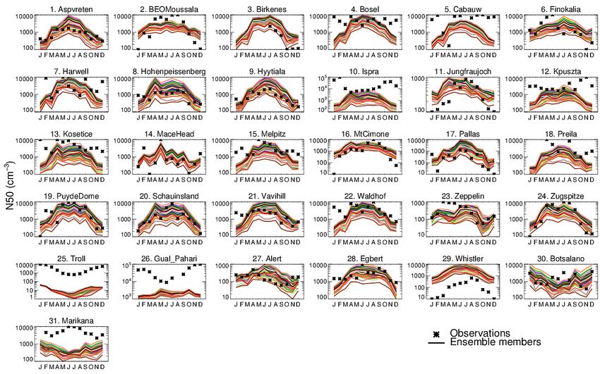
K. Sengupta et al.: A global model perturbed parameter ensemble study 2697
SOA (Donahue et al., 2011, 2012). Changing the ox-VOC pending strongly on the spatial heterogeneity of sources
concentrations by changing the yields of chemical reactions (Reddington et al., 2017).
has the same effect in the model as perturbing the emissions To examine the performance of the ensemble members,
of the parent VOCs. A yield above 100 % in the bimolecu- we use statistical metrics including correlation coefficient,
lar reactions should therefore be interpreted as an increase in normalized mean bias factor (NMBF), and Taylor skill score
the total concentration of reactants. The advantage of varying (TSS) (Taylor, 2001), in the following sections. NMBF is an
the yield of ox-VOCs rather than the emissions of VOCs is unbiased and symmetric metric with a range from −∞ to
that a perturbation applied to one ox-VOC does not affect the +∞, with 0 corresponding to exact agreement. It is calcu-
production or loss of the other ox-VOCs when they have the lated using the following equation:
same parent VOC (i.e. they have uncorrelated effects across PN
(Mi −Oi )
the 6-D parameter space). i=1
PN , if M̄ ≥ Ō
NMBF = PN (M i=1 Oi (1)
i −Oi )
i=1
PN , if M̄ < Ō,
2.5 Observations i=1 Mi
where for ensemble members i = {1, 2, . . .N }, Mi and Oi
Figure 3 shows a map of ground-based observation stations are the modelled and observed variables, the M̄ represents
used to compare the surface-level number concentrations of the mean across all ensemble members, and Ō represents
particles with dry diameter greater than 3 nm (N3 in recip- the mean across all observations. NMBF = 1.5(−1.5) means
rocal cubic centimetres), particles with dry diameter greater the model is biased towards overestimating (underestimat-
than 50 nm (N50 in reciprocal cubic centimetres) and the ing) observations by a factor of 2.5 (NMBF+1).
mass concentration of organic aerosol (OA in microgrammes The Taylor skill score (TSS) is calculated as
per cubic metre) predicted by the ensemble.
4(1 + R)4
N3 observations cover 34 ground stations worldwide as TSS = , (2)
used in Spracklen et al. (2010). Measurements of N3 were (σˆf + σ1ˆ )2 (1 + R0 )4
f
made between 1994 and 2009 using either condensation
particle counters (CPCs), scanning mobility particle sizers where σ̂ is the normalized standard deviation
(SMPSs), differential mobility particle sizers (DMPSs), or (σmodel /σobservation ), R is the Pearson correlation coeffi-
diffusion aerosol spectroscopes (DASs). The N3 data set is cient, and R0 is the maximum correlation attainable by the
fully described in Spracklen et al. (2010) and has been used model, assumed to be 1. As the model variance approaches
in previous studies such as Riccobono et al. (2014), Gor- the variance in the observations and R approaches R0 ,
don et al. (2016), and Dunne et al. (2016). N50 observa- i.e. the model is most skilful, TSS approaches unity. As
tions are from 31 ground stations worldwide including sites the model variance approaches zero or as the correlation
in Europe as described in Asmi et al. (2011) and at African coefficient between model and observation becomes more
(Vakkari et al., 2013), Indian (Hyvärinen et al., 2010), Cana- negative, TSS approaches zero. TSS thus takes into account
dian (Jeong et al., 2010; Takahama et al., 2011), and polar both how well the model simulates the observed pattern
(Asmi et al., 2016; Hansen et al., 2009) sites obtained from (correlation coefficient) and how close model observation
individual projects and online data portals. Measurements of agreement is (variance). The full statistics (TSS, NMBF, and
N50 were made between 2007 and 2015 using DMPS or R) calculated for each simulation within the ensemble is
SMPS instruments. OA observations cover 41 ground sta- presented in Table A1.
tions worldwide from the Global Aerosol Synthesis and Sci-
ence Project (GASSP) database (Reddington et al., 2017). 3 Results
OA measurements were made between 1990 and 2015 us-
ing the aerosol mass spectrometer (AMS) and the associated 3.1 Global and regional aerosol mass and number
aerosol chemical speciation monitor (ACSM) that character-
ize the mass and chemical composition of particulate matter The global mass of SOA produced in the model simulations
(Canagaratna et al., 2007; Ng et al., 2011). ranges from 220 to 850 Tg yr−1 across the 6-D parameter
All station data were averaged to create monthly mean range. Our global SOA range covers the upper end of the
values. Station heights were matched to model pressure lev- 50–380 Tg yr−1 global SOA found in Spracklen et al. (2011)
els for each month using barometric altitude. Stations cover after constraint of an earlier version of the GLOMAP model
a wide range of atmospheric conditions such as continen- to global AMS OA observations. Although individual ox-
tal boundary layer (CBL, e.g. Hyytiälä, Harwell, Botsalano), VOC yields were varied between 0 and 20 times their base-
marine boundary layer (MBL, e.g. Mace Head, Trinidad line yields, the total global production of SOA varies by only
Head, Sable Island), and free tropospheric (FT, e.g. Nepal, a factor of 4, and the lowest value is 220 Tg yr−1 . Global
Jungfraujoch, Pico Espejo, Mauna Loa) sites. Errors in mea- mean N50 varies by a factor of 2.39 within the ensemble
surements are estimated to be around 30 % on average, de- (from 377 to 903 cm−3 ). Modelled N3 is more sensitive to
https://doi.org/10.5194/acp-21-2693-2021 Atmos. Chem. Phys., 21, 2693–2723, 2021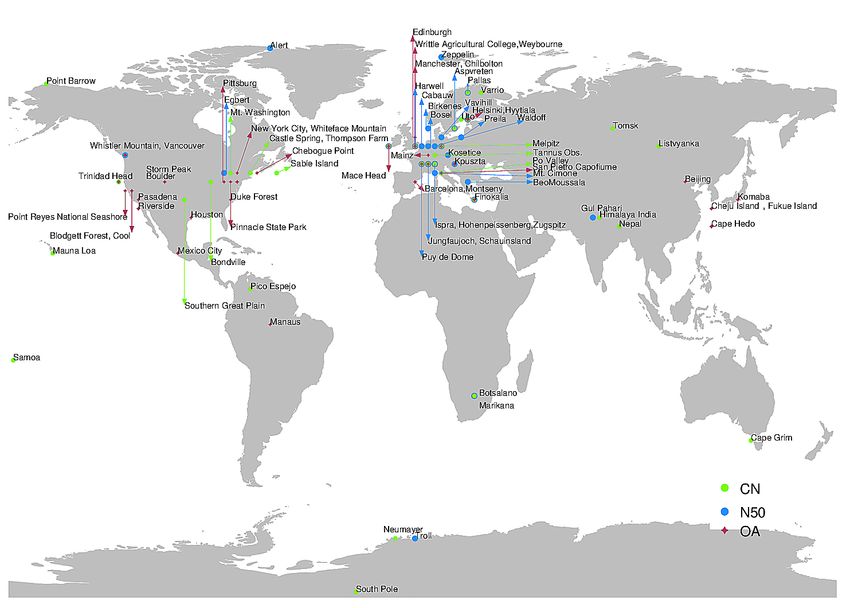
2698                                                   K. Sengupta et al.: A global model perturbed parameter ensemble study

Table 2. Perturbed parameters and ranges. Also listed are the precursor VOC gases that produce the ox-VOCs, the value of ox-VOC yields
in the default model version (unperturbed), how the perturbation for each parameter is implemented in the model (“absolute” for replacing
the default yield value by the perturbation, “scaled” for scaling the default yield value by the perturbation), and the amount of SOA produced
from each parameter in the default model version.

  Perturbed parameter                                                      Perturbation range                      Default SOA produced
  ox-VOC                  Produced                     Default yield   Minimum       Maximum        Perturbation            Tg(SOA) yr−1
                          from                            value (%)
  B_ELVOC                 Monoterpene, O3                        3.2            0    10 × default   scaled                               –
                          Monoterpene, OH q                      1.2            0    10 × default   scaled                               –
  B_LVOC                  Monoterpene, O3                         13            0    20 × default   absolute
                          Monoterpene, OH q                       13            0    20 × default   absolute                            16
                          Monoterpene, NO3 q                      13            0    20 × default   absolute
  B_SVOC_M                Monoterpene, O3                         13            0    20 × default   absolute
                          Monoterpene, OH q                       13            0    20 × default   absolute                            17
                          Monoterpene, NO3 q                      13            0    20 × default   absolute
  B_SVOC_I                Isoprene, O3                             3            0    20 × default   absolute
                          Isoprene, OH q                           3            0    20 × default   absolute                             6
                          Isoprene, NO3 q                          3            0    20 × default   absolute
  A_LVOC                  Anthropogenic VOC, OH q                 50            0    5 × default    absolute                            34
  A_SVOC                  Anthropogenic VOC, OH q                 50            0    5 × default    absolute                            34

changes in ox-VOCs than N50; global mean values vary by                  are predominantly biogenic in simulation 49 (Fig. 2). This
a factor of 3.5 across the 60 ensemble members (from 531 to              difference in parameter design is reflected in the global distri-
1889 cm−3 ).                                                             butions. Simulation 49 with low anthropogenic contributions
   Figure 4 shows that the ensemble members produce large                predicts lower OA concentrations in the highly polluted SE
regional variations in OA, even when they predict similar                Asian region. Anthropogenic ox-VOCs in the model favour
global values. For example, simulations 9 (subplot 4.3) and              the loss of smaller particles (which are more susceptible to
36 (subplot 5.3) have similar global mean OA concentra-                  condensation sinks) and the growth of larger particles (mass-
tions (6.47 and 6.49 µg m−3 respectively) but they simulate              based partitioning of A_SVOC). Therefore in the simulation
very different OA over the highly polluted regions of South              with low anthropogenic SOA more smaller particles survive
Asia. Such regional variations are dependent on the param-               but fewer particles hold substantial mass, leading to lower
eter settings of the ox-VOCs. In this case simulations 9 and             OA mass concentrations. This is also supported by the con-
36 particularly differ in the contribution from B_SVOC_M                 siderably higher N3 but only slightly higher N50 number
and A_LVOC. Modelling efforts need to focus on capturing                 concentrations in the SE Asian region in simulation 49 com-
the competing and compensating effects of ox-VOCs con-                   pared to simulation 45. Anthropogenic sources of SOA affect
tributing to different stages of particle formation and growth,          the pre-industrial and present-day atmospheres differently in
rather than detailed representation of any one contribution.             global models (Carslaw et al., 2013). Under-represented an-
This also emphasizes the need to compare model outputs                   thropogenic sources in global models therefore have greater
with regional as well as global metrics and observations to              climatic implications than under-represented biogenic SOA
determine whether the model is performing well.                          sources.
   Simulations 45 (subplot 2.9) and 49 (subplot 5.10) demon-                Figures 5 and 6 show the global distribution of N50 and
strate the role of anthropogenic VOCs on the simulated                   N3. The panels in each figure are ordered according to in-
aerosol size distribution and OA mass. Global mean N3,                   creasing global mean N3. There is a general increase in N50
N50, and OA in simulations 45 and 49 are all in the up-                  with increasing N3, but 11 of the simulations clearly show
per quartile of the ensemble’s output distribution for these             low N50 concentrations despite high N3 (simulations 14, 39,
quantities. Both of these simulations have high concentra-               47, 56, 50, 38, 9, 15, 59, 51 in Fig. 6). All of these simulations
tions of B_ELVOC, which promotes nucleation, and moder-                  have one aspect in common – very low yields of B_LVOC
ate to high B_LVOC, which promotes the survival of nucle-                (Fig. 2). High concentrations of nucleating B_ELVOC in
ated particles, contributing to the high global mean particle            these simulations initially facilitate the formation of par-
number and mass concentrations. In simulation 45 both bio-               ticles, but low yields of B_LVOC, especially when cou-
genic and anthropogenic ox-VOCs contribute significantly,                pled with one or more of high B_SVOC_I, A_LVOC, and
with B_ELVOC, B_SVOC_I, and A_LVOC concentrations                        A_SVOC, suppress particle growth up to 50 nm. B_SVOC_I,
being predominant (Fig. 2). In contrast contributions to SOA             A_LVOC, and A_SVOC are not spatially co-located with the

Atmos. Chem. Phys., 21, 2693–2723, 2021                                                     https://doi.org/10.5194/acp-21-2693-2021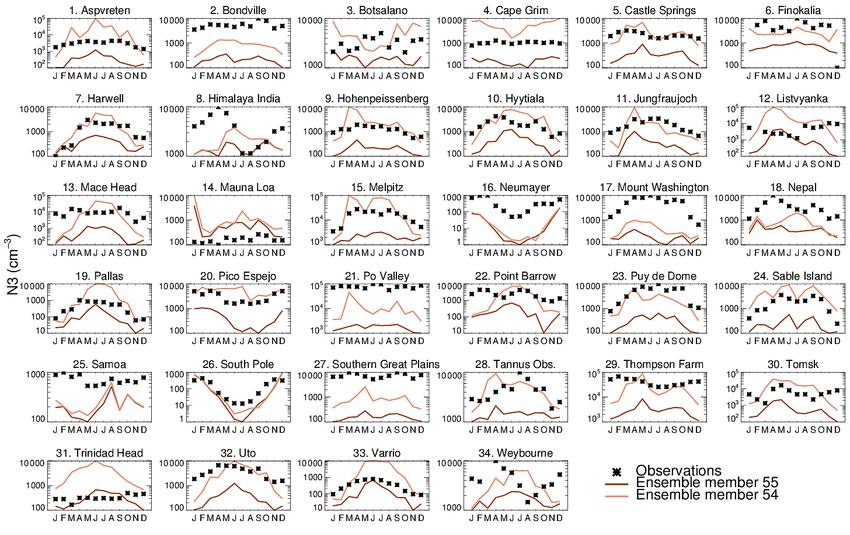
K. Sengupta et al.: A global model perturbed parameter ensemble study                                                                 2699

Figure 2. The relative variation in the six perturbed parameters (%) for each ensemble member (numbered 1 to 60). Each hexagon (grey
dashed area) represents the 6-D parameter space and the positions of the black dots show the position of each parameter within its range for
the specific ensemble member. The dots are joined and shaded green for easy identification of explored parameter space in each ensemble
member. Anticlockwise from top, the black dots represent parameter settings for B_ELVOC, B_LVOC, B_SVOC_M, B_SVOC_I, A_LVOC,
and A_SVOC respectively. Example interpretation: in simulation 19 (fourth row, first hexagon) B_SVOC_I and A_SVOC concentrations are
towards the lower ends of the respective ranges being explored for each of them while concentrations of A_LVOC are towards the high end
of the A_LVOC range.

nucleated clusters produced from biogenic ox-VOCs and fa-               spite the low B_ELVOC concentrations, which produces
cilitate the growth of larger particles, which then increases           fewer nucleated particles, the relatively high concentration of
the condensation sink for nucleated clusters, thereby effec-            B_LVOC ensures that more of the nucleated particles reach
tively suppressing the growth of nucleated clusters to N50-             50 nm diameter in these simulations. Consequently for these
relevant sizes in the above simulations with low B_LVOC                 simulations the simulated global mean N3 concentrations are
yields.                                                                 in the lower quartile within the ensemble but global mean
   In contrast, simulations 13, 24, 35, and 46 have low con-            N50 concentrations are in the interquartile range within the
centrations of B_ELVOC but relatively high B_LVOC. De-                  ensemble. B_LVOC can compensate for B_ELVOC to some

https://doi.org/10.5194/acp-21-2693-2021                                                   Atmos. Chem. Phys., 21, 2693–2723, 2021
2700                                               K. Sengupta et al.: A global model perturbed parameter ensemble study

Figure 3. Locations of ground-based sites where model–observation match is compared for N3 (34 locations, symbols in light), N50 (31
locations, symbols in blue), and OA (41 locations, symbols in red).

extent and clearly stands out as the most important controller      dicated by light shade). The colour coding clearly shows the
of climate-relevant particle number concentrations.                 multi-variate relationship between simulated N50, OA, and
   Including new, more accurate nucleation pathways into            ox-VOC parameters. High values of OA may be associated
models is unlikely to improve the model performance with            with various combinations of ox-VOC parameters and with
respect to N50 (a highly relevant model output for estimation       both high or low particle number concentrations. The fig-
of climate-relevant aerosol–cloud interactions) unless the          ure is consistent with the challenge faced by state-of-the-
models also include adequate representation of B_LVOCs.             art global models – despite simulating the particle number
Several studies have investigated nucleation capability and         concentrations (N3 and N50) reasonably well models con-
nucleation pathways of atmospheric molecules (Kulmala               sistently under-predict OA mass concentrations (Kanakidou
et al., 1998, 2004; Kirkby et al., 2011; Kurtén et al., 2008;       et al., 2005; Tsigaridis et al., 2014). The challenge in pre-
Almeida et al., 2013; Riccobono et al., 2014; Kirkby et al.,        dicting both particle number concentrations and OA mass is
2016), whereas the contribution of organic molecules to sub-        re-visited in later sections.
3 nm cluster growth is relatively recent knowledge, and the            N50 concentrations in Fig. 7 have a strong relationship
molecules involved are largely unidentified (Tröstl et al.,         with B_ELVOC up to about 5 times the ELVOC yield of
2016). The significance of B_LVOC is explored and estab-            3.2 % (Kirkby et al., 2016) used in the model, above which
lished further in later sections.                                   there is more scatter in N50 caused by the other model pro-
   Figure 7 shows how the global mean N50 and OA concen-            cesses and parameters. N50 is also related to B_LVOC, but
trations depend on the six ox-VOC parameters. The shad-             with more scatter than for B_ELVOC. These relationships
ing, blue for OA and red for N50, indicate whether the              show that N50 concentrations are strongly controlled in part
global mean values within the ensemble fall in the upper            by the production of B_ELVOC, which causes nucleation,
quartile (Q4 indicated by dark shade), inter-quartile range         and by the production of B_LVOC, which grows the nucle-
(IQR indicated by medium shade), or lower quartile (Q1 in-          ated clusters via kinetic condensation. There is no clear rela-

Atmos. Chem. Phys., 21, 2693–2723, 2021                                               https://doi.org/10.5194/acp-21-2693-2021
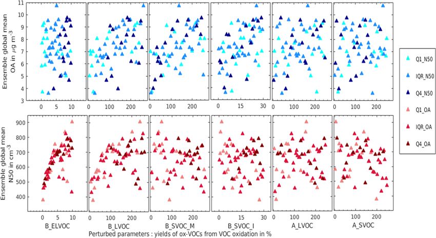
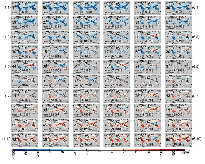
K. Sengupta et al.: A global model perturbed parameter ensemble study                                                         2701

Figure 4. Global annual mean anomaly of organic aerosol mass at the surface (OA in microgrammes per cubic metre) produced within the
ensemble. Each subplot shows the anomaly of an ensemble member (numbered between 1 and 60) from the ensemble mean OA. The global
mean OA is given on each subplot. The subplots are arranged in order of increasing global mean OA.

tionship between N50 and A_LVOC production. The likely              are more than 7.5 times the baseline yield of 13 % (above
reason for this is that anthropogenic VOCs are not spatially        100 % in Fig. 7; producing over 113 Tg yr−1 each).
co-located with the biogenically produced B_ELVOC, so                  We make two more observations from Fig. 7. The simu-
there are fewer nuclei in polluted regions and hence much           lated OA mass concentrations seem to have a stronger re-
less effect of the A_LVOC on the growth of nuclei to larger         lationship with SVOCs than LVOCs, because SVOCs parti-
sizes.                                                              tion to larger particles which already hold substantial mass,
   OA concentrations in Fig. 7 are found to be unrelated            thereby having a greater impact on OA mass. Secondly OA
to B_ELVOC concentration, showing that new particle for-            concentrations appear to have a steeper increase with in-
mation has little effect on simulated OA mass in our                creases in the biogenic ox-VOCs than their anthropogenic
model. Increases in all the other ox-VOC parameters gen-            counterparts. This is because in the current SOA scheme
erally increase OA, although there is a lot of scatter, par-        A_LVOCs or A_SVOCs grow fewer particles than their bio-
ticularly with the anthropogenic parameters, indicating a           genic counterparts which have the same spatial distribu-
strong multi-variate relationship for simulated OA. Global          tion as the nucleated particles they produce. As a result,
mean OA shows the strongest dependence on B_LVOC and                changes in the concentrations of anthropogenic ox-VOCs
B_SVOC_M, and the highest global mean OA (darkest red in            have a lesser impact on simulated OA mass. The involve-
Fig. 7) is simulated when B_LVOC and B_SVOC_M yields                ment of anthropogenic precursors in particle formation and

https://doi.org/10.5194/acp-21-2693-2021                                             Atmos. Chem. Phys., 21, 2693–2723, 2021
2702                                               K. Sengupta et al.: A global model perturbed parameter ensemble study

Figure 5. Global annual mean anomaly of N3 number concentration at the surface (cm−3 ) produced within the ensemble. Each subplot
shows the anomaly of an ensemble member (numbered between 1 and 60) from the ensemble mean N3. The global mean N3 is given on
each subplot. The subplots are arranged in order of increasing global mean N3.

cluster growth is likely to change this picture (Molteni et al.,   rest of the ox-VOCs (such as simulations 8, 21, 41, 54, and
2018).                                                             57), the increased competition between small particles for
   Overall we find that when particle number concentrations        growth cause the available high-volatility ox-VOCs to dis-
are low, the main difference between simulations that pro-         tribute on more particles, causing a smaller increase in the
duce a high amount of OA (simulations 16, 23, 35, and 46           particle mass.
in Fig. 4) and those that do not (see simulations 34, 55,
and 58 in Fig. 4) is the relative concentrations of B_LVOC,        3.2   Ensemble comparison with observations –
which grows freshly nucleated clusters before they can be                structural deficiencies in the model
scavenged by coagulation (see Fig. 2 for parameter combi-
nations). When particle number concentrations are high (due        Figure 8 shows the monthly-mean time series of N3 at 34
to high B_ELVOC or B_LVOC or both), the mass of OA pro-            ground sites. The 60-member ensemble is able to encompass
duced is determined by the combined effects of all other ox-       the observations in all months at only 3 out of 34 sites. In
VOCs. Parameter combinations such as in simulations 45 and         most locations the annual mean model bias in each of the
49 produce some of the highest global mean N3, N50, and            60 ensemble members ranges between a factor of 3 under-
OA within the ensemble. In parameter combinations in which         estimation to a factor of 2 overestimation, with underestima-
B_ELVOC and/or B_LVOC dominate significantly over the              tion being more prevalent. Riccobono et al. (2014), Dunne

Atmos. Chem. Phys., 21, 2693–2723, 2021                                             https://doi.org/10.5194/acp-21-2693-2021
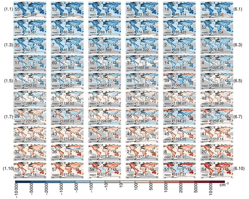
K. Sengupta et al.: A global model perturbed parameter ensemble study                                                       2703

Figure 6. Global annual mean anomaly of N50 number concentration at the surface (cm−3 ) produced within the ensemble. Each subplot
shows the anomaly of an ensemble member (numbered between 1 and 60) from the ensemble mean N50. The global mean N50 is given on
each subplot. The subplots are arranged in order of increasing global mean N3.

et al. (2016), and Gordon et al. (2016) have previously re-        and a factor of 2 overestimation, with underestimation be-
ported underestimation of wintertime particle number con-          ing more prevalent. The correlation coefficients (calculated
centrations by the model. Here we find the wintertime under-       for each ensemble member at each location using monthly
estimation continues even when B_ELVOC or B_LVOC ox-               mean simulated and observed N50 concentrations) in 22 out
VOC parameters are at their highest settings. In addition to       of 31 sites are higher than 0.5 (figure not shown). The best
underestimation of modelled concentrations in winter, some         correlation coefficients are observed in non-urban sites and
ensemble members overestimate particle concentration in the        the maximum underestimation and poorest correlation coef-
summer (for example Aspvreten in Fig. 8). These combined           ficients for N50 are observed at the polluted sites of Ispra
biases mean that the model overestimates the strength of           and Marikana (Asmi et al., 2011; Vakkari et al., 2013). In
the seasonal cycle compared to observations (see Appendix          contrast the ensemble performs significantly better at Hohen-
Figs. A1 and A2).                                                  peissenberg and Zugspitze, both high-altitude sites free from
   Figure 9 shows the monthly-mean time series of N50 at           nearby anthropogenic influence only about 458 km from Is-
31 ground sites. The 60-member ensemble is able to encom-          pra, and at Botsalano, representing a semi-clean environ-
pass the observations in all months at only 2 out of 31 sites.     ment, which is about 150 km from Marikana.
Like N3, the model bias for N50 in each of the 60 ensem-              We also find that as the normalized mean bias factor (cal-
ble members ranges between a factor of 3 underestimation           culated between each simulation and observed values) de-

https://doi.org/10.5194/acp-21-2693-2021                                            Atmos. Chem. Phys., 21, 2693–2723, 2021
2704 K. Sengupta et al.: A global model perturbed parameter ensemble study
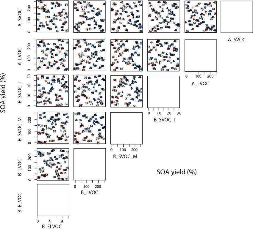
Figure 7. Global annual mean OA (top panel) and N50 (bottom panel) against the perturbed range of the six ox-VOCs for the 60 ensemble
members. The three shades of blue in the top panel divide the ensemble members into three categories according to the mean N50 concen-
trations: Q1_N50 for N50 values in the lower quartile, IQR_N50 for the inter-quartile range, and Q4_N50 for N50 values in the the upper
quartile. The three shades of red in the bottom panel depict the same as above but for global mean OA concentrations in the ensemble.
creases, the calculated correlation coefficient weakens. This to the baseline model yields (Table 2) to get the B_ELVOC
implies that the model has a structural deficiency that cannot yields for the ensemble members. For the rest of the ox-
be resolved by perturbing the model parameters. The strong VOCs the values shown are yield values in percent which can
link between B_ELVOC and N3 indicates that the weaken- be converted to teragrammes per year using Table 2. Because
ing of the correlation coefficient with the improvement of it is a 6-D space, it is also important to note that the other four
normalized mean bias factor is related to nucleation: higher parameters are varying randomly across each plane.
ELVOC production rates increase annual mean N3 concen- We use Figs. 10, 11, and 12 to identify patterns of depen-
trations, but the summer concentrations are affected much dencies of the Taylor skill scores for N3, N50, and OA on
more than the winter concentrations, which weakens the cor- the ox-VOC yields within the 6-D parameter space. A weak
relation. We suggest that a missing particle source such as dependency between an ox-VOC and model skill does not
anthropogenic pollutants – which are at a maximum in the imply that the contribution of the ox-VOC to OA and parti-
winter due to low boundary layer height and increased lo- cle number concentration is unimportant. Rather, it implies
cal emissions from sources such as domestic heating – will that within the current modelling framework its contribution
rectify the model bias significantly. Alternatively, the poor can be compensated for by changes in other ox-VOCs.
model performance may be improved by exploring uncer- To identify the plausible and implausible parts of the pa-
tainties in other parts of the model unrelated to SOA (Lee rameter space using the patterns of dependencies, the ensem-
et al., 2013; Yoshioka et al., 2019). ble simulations (denoted by triangles in Figs. 10, 11, and 12)
in the subplots are shaded blue to red. Darker shades of blue
3.3 Model skill across the 6-D parameter space indicate low/poor Taylor skill score and darker shades of red
represent high/good Taylor skill score within the ensemble.
We now explore how the model skill in simulating observed We note the relative rank of the simulations in Taylor skill
N3, N50, and OA varies across the 6-D ox-VOC parameter score and their relative positions in each 2-D subplot and use
space (Figs. 10, 11, and 12). Each scatter plot in Figs. 10, this information to identify clusters of blue or red triangles
11, and 12 shows the relationship between two ox-VOCs in the parameter space. For absolute values of Taylor skill
for each of the 60 ensemble members. Note the values for scores of each simulation, see Table A1 and Figs. A3, A4,
B_ELVOC yields shown in Figs. 10, 11, and 12 and Figs. A3, and A5 (which are Figs. 10, 11, and 12 labelled with simula-
A4, and A5 are scaling factors which have to be multiplied tion number).
Atmos. Chem. Phys., 21, 2693–2723, 2021 https://doi.org/10.5194/acp-21-2693-2021K. Sengupta et al.: A global model perturbed parameter ensemble study 2705
Figure 8. Seasonal cycle of simulated (solid coloured lines) and observed (black stars) monthly mean surface-level N3 concentrations at 34
ground-based sites. Each coloured line is an ensemble member.
Some clear patterns in model skill are apparent across the N50 skill has the strongest dependency on B_LVOC. The
six dimensions. N3 skill depends strongly on B_ELVOC, model is most skilful (clusters of red triangles) for B_LVOC
B_LVOC, and A_LVOC (Fig. 10). The skill is generally greater than about 113 Tg yr−1 (corresponding to a yield of
lower (clusters of blue triangles) for B_ELVOC yields less 100 %, Fig. 11 second column) with a general increase in
than 6.4 % from ozonolysis of α-pinene (i.e. twice the base- skill for higher values of B_LVOC. N50 skill is generally
line yield; see Fig. 10 first column, fifth row), irrespective of lower (blue triangles) for B_ELVOC yields less than twice
the value of other parameters (left column in Fig. 10). The N3 the baseline yield or 6.4 %, although other parameter values
skill is also generally low for values of A_LVOC greater than and particularly high B_LVOC improve model skill in some
about 95 Tg yr−1 (yield corresponding to 150 % in Fig. 10), cases (Fig. 11 first column, fifth row; note the cluster of red
although there are a few simulations that have reasonable triangles in the top left corner of the subplot compared to the
skill (triangles in lighter shades of red amidst mostly blue tri- same area in the subplots above). The dependence of N50
angles) above this value (Fig. 10 second row). We note two skill on A_LVOC is much weaker than for N3, with high and
additional regions in the 6-D space dominated by low model low model skills spread across the entire parameter range. In
skill in N3 – where B_ELVOC yield is greater than 19.8 % contrast the N50 skill tends to be low for A_SVOCs greater
and B_LVOC is less than 113 Tg yr−1 (Fig. 10 first column, than about 95 Tg yr−1 (150 % yield, Fig. 11 first row).
fifth row, cluster of blue triangles in the bottom right corner Figures 10 and 11 show that model simulation of N3 and
of the subplot corresponding to 6 times the baseline yield on N50 is most skilful when B_ELVOC production is a fac-
the x axis and a yield of 100 % on the y axis) and where tor of 2 to 8 higher than the baseline model B_ELVOC
the sum of anthropogenic LVOC and SVOC is greater than yields of 3.2 % and 1.2 % from O3 and OH q oxidation reac-
127 Tg yr−1 (Fig. 10 fifth column, first row, cluster of blue tions respectively (Kirkby et al., 2016). With less than 6.4 %
triangles in the top right corner of the subplot correspond- B_ELVOC yields from O3 and OH q oxidation reactions,
ing to 200 % yield on both x and y axes). There is also a the model–observation match is consistently poor (shades of
general increase in skill for high values of B_LVOC (second blue in Figs. 10 or 13). The best estimate of B_ELVOC yield
column). to obtain reasonable agreement with observed N3, N50, and
OA in our model (denoted by shades of red in Fig. 13) is
https://doi.org/10.5194/acp-21-2693-2021 Atmos. Chem. Phys., 21, 2693–2723, 20212706 K. Sengupta et al.: A global model perturbed parameter ensemble study Figure 9. Seasonal cycle of simulated (solid coloured lines) and observed (black stars) monthly mean surface-level N50 concentrations at 31 ground-based sites. Each coloured line is an ensemble member. about a factor of 4 higher than the baseline B_ELVOC yield nality is that fine-tuning any one aspect of the model (for from ozonolysis of α-pinene (Kirkby et al., 2016). example, the nucleation mechanism) to achieve best model– OA skill has the strongest joint dependency on B_LVOC observation agreement for any one variable (e.g. the particle and B_SVOC_M (Fig. 12). The joint distribution suggests number concentration) can be achieved with a wide range that the skill is poor if the sum of these SOA production rates of settings of other parameters (e.g. parameters controlling exceeds about 226 Tg yr−1 (up to 200 % yield of both; Fig. 12 overall OA mass production). While this may not affect the second column, fourth row). However, for all other parame- overall model skill in the particular evaluation, the various ters there are skilful and unskillful simulations right across parts of equally plausible parameter space may result in very the 6-D parameter space. different model behaviour in, say, climate projections. Together, the variations in skill for N3, N50, and OA con- Figure 13 summarizes Figs. 10, 11, and 12 showing the centrations across the six dimensions show that the parame- model skill score in all three model outputs across the entire ter space for a high N3 or N50 skill score does not overlap parameter space for all six ox-VOCs in 1-D. We find five with the parameter space for a high OA skill score (Figs. 10, simulations that are shaded red for all three model outputs 11, and 12). This gives an insight as to why models that are across the six parameters: simulations 8, 17, 19, 21, and 41. fine-tuned to simulate particle number concentrations under- The parameter combinations and the resulting Taylor skill estimate OA mass concentrations in the atmosphere – also scores are listed in Tables 3 and A2. identified as a persistent challenge for state-of-the-art global One ensemble member, simulation 41, scores reasonably models (Kanakidou et al., 2005; Spracklen et al., 2011). well (Taylor skill scores of 0.28, 0.11, and 0.14 for N3, N50, Our results reveal the problem of model equifinality, high- and OA) in simulating observed mass and number of parti- lighted for the whole aerosol model by Lee et al. (2016). cles. It is the only simulation for which Taylor skill score Equifinality means that there are multiple ways (i.e. parame- in each of the three outputs is among the top 10 highest ter combinations) of achieving the same model skill against scores within the ensemble (see Table A1). The score is high- observations, which makes it difficult to identify the best est for N3, second highest for N50 (0.12 being the high- model (Beven, 2006). An important consequence of equifi- est score), and sixth highest for OA (0.19 being the high- Atmos. Chem. Phys., 21, 2693–2723, 2021 https://doi.org/10.5194/acp-21-2693-2021
K. Sengupta et al.: A global model perturbed parameter ensemble study                                                                     2707

Figure 10. Taylor skill score for model simulations against N3 observations across the 6-D parameter space. The x and y axes for a subplot
show the total range of reaction yields (%) over which each of the two parameters (as indicated by the plot labels at the top and right for each
subplot respectively) is perturbed in the ensemble. Each triangle in a subplot represents a simulation, and the color of the triangle indicates
its Taylor skill score for N3. Darker shades of blue indicate low/poor Taylor skill score and darker shades of red represent high/good Taylor
skill score. Figure A3 shows the same plot with ensemble members numbered. Note the axis for B_ELVOC shows the scaling factor for
B_ELVOC yields. Axes for the rest show the corresponding ox-VOC yields.

Table 3. Yield of B_ELVOC and SOA (Tg yr−1 ) for other ox-VOCs with the corresponding Taylor skill scores for five ensemble members
that are shaded red for all three outputs N3, N50, and OA in Fig. 13. The parameter combinations used to produce the above ox-VOCs in the
ensemble are listed in Table A2.

         PPEM              B_ELVOC        B_LVOC       B_SVOC_M         B_SVOC_I       A_LVOC       A_LVOC         N3     N50     OA
                    % yield O3 (OH q)                              Tg yr−1 of SOA                                  Taylor skill score
         8                  20.5 (7.7)      122.72            59.76           31.89        43.55        64.96     0.23    0.10   0.15
         17                  9.7 (3.6)      178.15            74.25           49.27        75.89        73.15     0.23    0.10   0.12
         19                 13.8 (5.2)      121.96           136.20           10.83       108.49        10.55     0.23    0.10   0.13
         21                 23.9 (8.9)      226.26             42.2            4.65        96.24        87.28     0.22    0.11   0.13
         41                 13.2 (4.9)       157.7            17.49           16.02        38.09        13.48     0.28    0.11   0.14

https://doi.org/10.5194/acp-21-2693-2021                                                     Atmos. Chem. Phys., 21, 2693–2723, 2021
2708 K. Sengupta et al.: A global model perturbed parameter ensemble study
Figure 11. Taylor skill score for model simulations against N50 observations across the 6-D parameter space. The x and y axes for a subplot
show the total range of reaction yields (%) over which each of the two parameters (as indicated by the plot labels at the top and right for each
subplot respectively) is perturbed in the ensemble. Each triangle in a subplot represents a simulation and the color of the triangle indicates
its Taylor skill score for N50. Darker shades of blue indicate low/poor Taylor skill score and darker shades of red represent high/good Taylor
skill score. Figure A4 shows the same plot with ensemble members numbered. Note the axis for B_ELVOC shows the scaling factor for
B_ELVOC yields. Axes for the rest show the corresponding ox-VOC yields.
est score). For this simulation B_ELVOC is 4.1 times the N50, and OA, simulation 41 has much scope for improve-
baseline yield (i.e. about 13 % B_ELVOC yield from O3 ment. Nevertheless it exemplifies the characteristics required
and 5 % yield from OH q), with about 157 Tg yr−1 of SOA to improve the simulation of SOA in the model.
from B_LVOC, 33 Tg yr−1 from B_SVOC (monoterpenes
+ isoprene), 38 Tg yr−1 from A_LVOC, and 13 Tg yr−1
from A_SVOC. In this simulation the SOA production path- 4 Conclusions
ways are characterized by (i) high concentrations of both
B_ELVOC and B_LVOC that ensure particle production We have used a perturbed parameter ensemble of 60 model
via nucleation and subsequent growth of nucleated clusters, simulations to explore how uncertainty in six biogenic and
(ii) relatively high A_LVOC concentrations that further help anthropogenic precursors affects organic aerosol mass and
to sustain the growth of small particles in the nucleation particle number concentrations. The ranges for each parame-
mode, and (iii) modest yields of SVOCs that ensure effective ter were chosen to encompass maximum uncertainty associ-
growth of particles up to sizes relevant to cloud condensation ated with organic compounds that affect three different stages
nuclei (CCN), improving skill scores for N50 and OA, while of SOA formation − nucleation, cluster growth, and particle
at the same time restraining the condensation sink and the growth. Simultaneous perturbations of the six parameters us-
loss of too many growing particles by coagulation scaveng- ing a Latin hypercube sampling technique allow the effects
ing. With Taylor skill scores of 0.28, 0.11, and 0.14 for N3, of parameter combinations rather than just individual param-
eters on model outputs to be explored. Three model outputs,
Atmos. Chem. Phys., 21, 2693–2723, 2021 https://doi.org/10.5194/acp-21-2693-2021K. Sengupta et al.: A global model perturbed parameter ensemble study 2709 Figure 12. Taylor skill score for model simulations against OA observations across the 6-D parameter space. The x and y axes for a subplot show the total range of reaction yields (%) over which each of the two parameters (as indicated by the plot labels at the top and right for each subplot respectively) is perturbed in the ensemble. Each triangle in a subplot represents a simulation and the color of the triangle indicates its Taylor skill score for OA. Darker shades of blue indicate low/poor Taylor skill score and darker shades of red represent a high/good Taylor skill score. Figure A5 shows the same plot with ensemble members numbered. Note the axis for B_ELVOC shows the scaling factor for B_ELVOC yields. Axes for the rest show the corresponding ox-VOC yields. the number concentration of particles larger than 3 nm diam- ELVOC, LVOC, and SVOC. B_ELVOC is crucial for the for- eter (N3), the number concentration of particles larger than mation of particles via nucleation. Thereafter contributions 50 nm diameter (N50), and the organic aerosol (OA) mass from LVOCs and SVOCs contribute to the growth of freshly- concentration, were compared against observations, and the nucleated particles to produce a realistic N50 concentration model skill score was then used to determine the skilful parts and SOA mass. of parameter space. B_ELVOC strongly influences model skill scores in N3 The results expose a high degree of equifinality in the SOA and to a lesser extent in N50 Fig. 13). When B_ELVOC model in which there are multiple ways of generating simi- is low (< twice the baseline yield of 3.2 %), the ensem- lar outputs (particle concentrations and OA mass). This is to ble consistently underestimates N3 and N50 number concen- be expected in a system with six free parameters and only trations, irrespective of the availability of other ox-VOCs. three output variables of interest – that is, our six-component We find the best model skill scores in N3, N50, and OA SOA model is underdetermined. Equifinality, or compensat- are achieved when the ELVOC yield from precursor VOCs ing parameter effects, limit the extent to which the best set of is between 6–26 %, with the most plausible ELVOC yield parameters can be identified by comparing the simulations estimate being around 12.8 %. Previously reported ELVOC against observations. Our results suggest that the effects of yields from α-pinene ozonolysis are at the lower end of three categories of volatile organic compounds can be de- this constrained range (3.2 % with an uncertainty range of tected by comparing the 60 simulations against observations: +100 %/−60 % reported by Kirkby et al. (2016), 7 ± 4 % https://doi.org/10.5194/acp-21-2693-2021 Atmos. Chem. Phys., 21, 2693–2723, 2021
You can also read