Optimal Trajectory Planning for Cinematography with Multiple Unmanned Aerial Vehicles
←
→
Page content transcription
If your browser does not render page correctly, please read the page content below
Optimal Trajectory Planning for Cinematography
                                                                 with Multiple Unmanned Aerial Vehicles
                                                                           Alfonso Alcantaraa , Jesus Capitana , Rita Cunhab , Anibal Olleroa
                                                                                            a GRVC Robotics Laboratory, University of Seville, Spain.
                                                                    b Institute   for Systems and Robotics, Instituto Superior Tcnico, Universidade de Lisboa, Portugal.

                                        Abstract
                                        This paper presents a method for planning optimal trajectories with a team of Unmanned Aerial Vehicles (UAVs) performing
                                        autonomous cinematography. The method is able to plan trajectories online and in a distributed manner, providing coordination
arXiv:2009.04234v1 [cs.RO] 9 Sep 2020

                                        between the UAVs. We propose a novel non-linear formulation for this challenging problem of computing multi-UAV optimal
                                        trajectories for cinematography; integrating UAVs dynamics and collision avoidance constraints, together with cinematographic
                                        aspects like smoothness, gimbal mechanical limits and mutual camera visibility. We integrate our method within a hardware and
                                        software architecture for UAV cinematography that was previously developed within the framework of the MultiDrone project; and
                                        demonstrate its use with different types of shots filming a moving target outdoors. We provide extensive experimental results both
                                        in simulation and field experiments. We analyze the performance of the method and prove that it is able to compute online smooth
                                        trajectories, reducing jerky movements and complying with cinematography constraints.
                                        Keywords: Optimal trajectory planning, UAV cinematography, Multi-UAV coordination

                                        1. Introduction                                                                   potential obstacles, keeping other cameras out of the field of
                                                                                                                          view, etc.
                                           Drones or Unmanned Aerial Vehicles (UAVs) are spreading                           There exist commercial products (e.g., DJI Mavic [1] or Sky-
                                        fast for aerial photography and cinematography, mainly due to                     dio [2]) that cope with some of the aforementioned complexi-
                                        their maneuverability and their capacity to access complex film-                  ties implementing semi-autonomous functionalities, like auto-
                                        ing locations in outdoor settings. From the application point of                  follow features to track an actor or simplistic collision avoid-
                                        view, UAVs present a remarkable potential to produce unique                       ance. However, they do not address cinematographic principles
                                        aerial shots at reduced costs, in contrast with other alternatives                for multi-UAV teams, as e.g., planning trajectories considering
                                        like dollies or static cameras. Additionally, the use of teams                    gimbal physical limitations or inter-UAV visibility. Therefore,
                                        with multiple UAVs opens even more the possibilities for cin-                     solutions for autonomous filming with multiple UAVs are of in-
                                        ematography. On the one hand, large-scale events can be ad-                       terest. Some authors [3] have shown that planning trajectories
                                        dressed by filming multiple action points concurrently or se-                     ahead several seconds is required in order to fulfill with cine-
                                        quentially. On the other hand, the combination of shots with                      matographic constraints smoothly. Others [4, 5] have even ex-
                                        multiple views or different camera motions broadens the artis-                    plored the multi-UAV problem, but online trajectory planning
                                        tic alternatives for the director.                                                for multi-UAV cinematography outdoors is still an open issue.
                                           Currently, most UAVs in cinematography are operated in                            In this paper, we propose a method for online planning and
                                        manual mode by an expert pilot. Besides, an additional quali-                     execution of trajectories with a team of UAVs taking cine-
                                        fied operator is required to control the camera during the flight,                matography shots. We develop an optimization-based tech-
                                        as taking aerial shots can be a complex and overloading task.                     nique that runs on the UAVs in a distributed fashion, taking
                                        Even so, the manual operation of UAVs for aerial cinematog-                       care of the control of the UAV and the gimbal motion simul-
                                        raphy is still challenging, as multiple aspects need to be con-                   taneously. Our method aims at providing smooth trajectories
                                        sidered: performing smooth trajectories to achieve aesthetic                      for visually pleasant video output; integrating cinematographic
                                        videos, tracking actors to be filmed, avoiding collisions with                    constraints imposed by the shot types, the gimbal physical lim-
                                                                                                                          its, the mutual visibility between cameras and the avoidance of
                                                                                                                          collisions.
                                           I This work was partially funded by the European Union’s Horizon 2020
                                                                                                                             This work has been developed within the framework of the
                                        research and innovation programme under grant agreements No 731667 (Mul-
                                        tiDrone), and by the MULTICOP project (Junta de Andalucia, FEDER Pro-
                                                                                                                          EU-funded project MultiDrone1 , whose objective was to create
                                        gramme, US-1265072).                                                              a complete system for autonomous cinematography with multi-
                                             Email addresses: aamarin@us.es (Alfonso Alcantara),
                                        jcapitan@us.es (Jesus Capitan), rita@isr.utl.pt (Rita Cunha),
                                        aollero@us.es (Anibal Ollero)                                                         1 https://multidrone.eu.
like classic PID [17] or LQR [18] controllers. The main issues
                                                                                  with all these methods for trajectory planning and target track-
                                                                                  ing are that they either do not consider cinematographic aspects
                                                                                  explicitly or do not plan ahead in time for horizons long enough.
                                                                                     In the computer animation community, there are several
                                                                                  works related with trajectory planning for the motion of vir-
                                                                                  tual cameras [19]. They typically use offline optimization to
                                                                                  generate smooth trajectories that are visually pleasant and com-
                                                                                  ply with certain cinematographic aspects, like the rule of thirds.
                                                                                  However, many of them do not ensure physical feasibility to
                                                                                  comply with UAV dynamic constraints and they assume full
                                                                                  knowledge of the environment map. In terms of optimiza-
                                                                                  tion functions, several works consider similar terms to achieve
                                                                                  smoothness. For instance, authors in [20] model trajectories
                                                                                  as polynomial curves whose coefficients are computed to min-
                                                                                  imize snap (fourth derivative). They also check dynamic feasi-
                                                                                  bility along the planned trajectories, and the user is allowed to
Figure 1: Cinematography application with two UAVs filming a cycling event.       adjust the UAV velocity at execution time. A similar applica-
Bottom, aerial view of the experiment with two moving cyclists. Top, images
taken from the cameras on board each UAV.
                                                                                  tion to design UAV trajectories for outdoor filming is proposed
                                                                                  in [21]. Timed reference trajectories are generated from 3D po-
                                                                                  sitions specified by the user, and the final timing of the shots
ples UAVs in outdoor sport events (see Figure 1). MultiDrone                      is addressed designing easing curves that drive the UAV along
addressed different aspects to build a complete architecture: a                   the planned trajectory (i.e., curves that modify the UAV veloc-
set of high-level tools so that the cinematography director can                   ity profile). In [22], aesthetically pleasant footage is achieved
define shots for the mission [6]; planning methods to assign and                  by penalizing the snap of the UAV trajectory and the jerk (third
schedule the shots among the UAVs efficiently and considering                     derivative) of the camera motion. An iterative quadratic opti-
battery constraints [7]; vision-based algorithms for target track-                mization problem is formulated to compute trajectories for the
ing on the camera image [8], etc. In this paper, we focus on the                  camera and the look-at point (i.e., the place where the camera is
autonomous execution of shots with a multi-UAV team. We as-                       pointing at). They also include collision avoidance constraints,
sume that the director has designed a mission with several shots;                 but the method is only tested indoors.
and that there is a planning module that has assigned a specific                     Although these articles on computer graphics approach the
shot to each UAV. Then, our objective is to plan trajectories in                  problem mainly through offline optimization, some of them
order to execute all shots online in a coordinated manner.                        have proposed options to achieve real-time performance, like
                                                                                  planning in a toric space [23] or interpolating polynomial
1.1. Related work                                                                 curves [24, 21]. In general, these works present interesting the-
   Optimal trajectory planning for UAVs is a commonplace                          oretical properties, but they are restricted to offline optimization
problem in the robotics community. A typical approach is                          with a fully known map of the scenario and static or close-to-
to use optimization-based techniques to generate trajectories                     static guided tour scenes, i.e., without moving actors.
from polynomial curves minimizing their derivative terms for                         In the robotics literature, there are works focusing more on
smoothness, e.g., the fourth derivative or snap [9, 10]. This                     filming dynamic scenes and complying with physical UAV con-
polynomial trajectories have also been applied to optimization                    straints. For example, authors in [25] propose to detect limbs
problems with multiple UAVs [11]. Model Predictive Control                        movement of a human for outdoor filming. Trajectory planning
(MPC) is another widespread technique for optimal trajectory                      is performed online with polynomial curves that minimize snap.
planning [12], a dynamic model of the UAV is used for predict-                    In [26, 3], they present an integrated system for outdoor cin-
ing and optimizing trajectories ahead within a receding hori-                     ematography, combining vision-based target localization with
zon. Some authors [13] have also used MPC-based approaches                        trajectory planning and collision avoidance. For optimal trajec-
for multi-UAV trajectory planning with collision avoidance and                    tory planning, they apply gradient descent with differentiable
non-linear models. In the context of multi-UAV target track-                      cost functions. Smoothness is achieved minimizing trajectory
ing, others [14, 15] have combined MPC with potential fields to                   jerk; and shot quality by defining objective curves fulfilling cin-
address the non-convexity induced by collision avoidance con-                     ematographic constraints associated with relative angles w.r.t.
straints. In [16], a constrained optimization problem is formu-                   the actor and shot scale. Cinematography optimal trajectories
lated to maintain a formation where a leader UAV takes pictures                   have also been computed in real time through receding horizon
for inspection in dark spaces, while others illuminate the target                 with non-linear constraints [27]. The user inputs framing ob-
spot supporting the task. The system is used for aerial docu-                     jectives for one or several targets on the image, and errors of
mentation within historical buildings.                                            the image target projections, sizes and relative viewing angles
   Additionally, there are works in the literature just for target                are minimized; satisfying collision avoidance constraints and
tracking with UAVs, proposing alternative control techniques                      target visibility. The method behaves well for online numerical
                                                                              2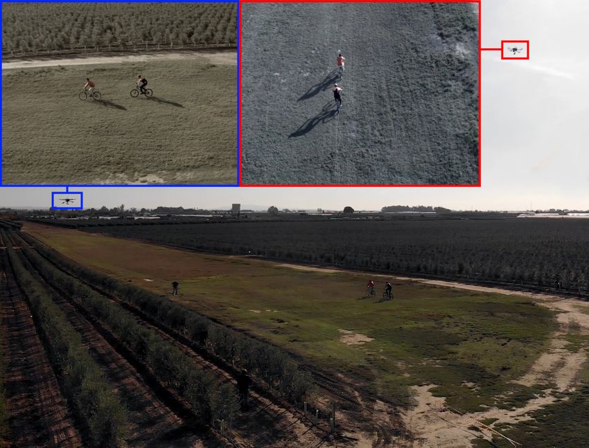
Figure 2: Related works on trajectory planning for UAV cinematography. We indicate whether computation is online or not, the type of scene and constraints they
consider, and their capacity to handle outdoor applications and multiples UAVs.

optimization, but it is only tested in indoor settings.                           (i) we cope with multiple UAVs integrating new constraints for
   Some of the aforementioned authors from robotics have also                     inter-UAV collisions and mutual visibility; (ii) we present ad-
approached UAV cinematography applying machine learning                           ditional simulation results to evaluate the method with differ-
techniques. In particular, learning from demonstration to imi-                    ent types of shots; and (iii) we demonstrate the system in field
tate professional cameraman’s behaviors [28] or reinforcement                     experiments with multiple UAVs filming dynamic scenes. In
learning to achieve visually pleasant shots [29]. In general,                     particular, our main contributions are the following:
most of these cited works on robotics present results quite inter-
esting in terms of operation outdoors or online trajectory plan-
                                                                                     • We propose a novel formulation of the trajectory planning
ning, but they always restrict to a single UAV.
                                                                                       problem for UAV cinematography. We model both UAV
   Regarding methods for multiple UAVs, there is some related
                                                                                       and gimbal motion (Section 2), but decouple their control
work which is worth mentioning. In [4], a non-linear optimiza-
                                                                                       actions.
tion problem is solved in a receding horizon fashion, taking into
account collision avoidance constraints with the filmed actors
and between the UAVs. Aesthetic objectives are introduced by                         • We propose a non-linear, optimization-based method for
the user as virtual reference trails. Then, UAVs receive current                       trajectory planning (Section 3). Using a receding hori-
plans from all others at each planning iteration and compute                           zon scheme, trajectories are planned and executed in a
collision-free trajectories sequentially. A UAV toric space is                         distributed manner by a team of UAVs providing multiple
proposed in [5] to ensure that cinematographic properties and                          views of the same scene. The method considers UAV dy-
dynamic constraints are ensured along the trajectories. Non-                           namic constraints, and imposes them to avoid predefined
linear optimization is applied to generate polynomial curves                           no-fly zones or collisions with others. Cinematographic
with minimum curvature variation, accounting for target vis-                           aspects imposed by shot definition, camera mutual visibil-
ibility and collision avoidance. The motion of multiple UAVs                           ity and gimbal physical bounds are also addressed. Trajec-
around dynamic targets is coordinated by means of a centralized                        tories smoothing UAV and gimbal motion are generated to
master-slave approach to solve conflicts. Even though these                            achieve aesthetic video footage.
works present promising results for multi-UAV teams, they are
only demonstrated at indoor scenarios where a Vicon motion                           • We describe the complete system architecture on board
capture system provides accurate positioning for all targets and                       each UAV and the different types of shot considered (Sec-
UAVs.                                                                                  tion 4). The architecture integrates target tracking with
   To sum up, Figure 2 shows a table with the main related                             trajectory planning and it is such that different UAVs can
works on trajectory planning for UAV cinematography and their                          be executing different types of shot simultaneously.
corresponding properties.

                                                                                     • We present extensive experimental results (Section 5) to
1.2. Contributions
                                                                                       evaluate the performance of our method for different types
   We propose a novel method to plan online optimal trajecto-                          of shot. We prove that our method is able to com-
ries for a set of UAVs executing cinematography shots. The                             pute smooth trajectories reducing jerky movements in real
optimization is performed in a distributed manner, and it aims                         time, and complying with the cinematographic restric-
for smooth trajectories complying with dynamic and cinemato-                           tions. Then, we demonstrate our system in field experi-
graphic constraints. We extend our previous work [30] in op-                           ments with three UAVs planning trajectories online to film
timal trajectory planning for UAV cinematography as follows:                           a moving actor (Section 6).
                                                                              3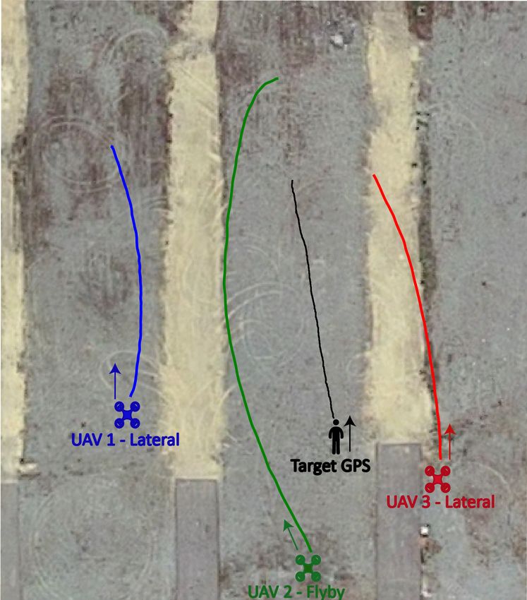
If we restrict the yaw angle ψQ to keep the quadrotor’s front
pointing forward in the direction of motion such that:
ψQ = atan2(vy , v x ), (3)
then the thrust T and the Z-Y-X Euler angles λQ =
[φQ , θQ , ψQ ]T can be obtained from vQ and aQ according to:
T = mkaQ + ge3 k
ψQ = atan2(vy , v x )
(4)
φQ = − arcsin((ay cos(ψQ ) − a x sin(ψQ ))/kaQ + ge3 k)
θQ = atan2(a x cos(ψQ ) + ay sin(ψQ ), az + g)
2.2. Gimbal angles
Figure 3: Definition of reference frames used. The origins of the camera and
quadrotor frames coincide. The camera points to the target.
Let λC = [φC , θC , ψC ]T denote the Z-Y-X Euler angles that
parametrize the rotation matrix RC , such that:
RC = Rz (ψC )Ry (θC )R x (φC ). (5)
2. Dynamic Models
In our system, we decouple gimbal motion with an indepen-
This section presents our dynamic models for UAV cine- dent gimbal attitude controller that ensures that the camera is
matographers. We model the UAV as a quadrotor with a camera always pointing towards the target during the shot, as in [3].
mounted on a gimbal of two degrees of freedom. This reduces the complexity of the planning problem and al-
lows us to control the camera based on local perception feed-
2.1. UAV model back if available, accumulating less errors. We also consider
that the time-scale separation between the ”faster” gimbal dy-
Let {W} denote the world reference frame with origin fixed
namics and ”slower” quadrotor dynamics is sufficiently large
in the environment and East-North-Up (ENU) orientation. Con-
to neglect the gimbal dynamics and assume an exact match be-
sider also three additional reference frames (see Figure 3): the
tween the desired and actual orientations of the gimbal. In order
quadrotor reference frame {Q} attached to the UAV with origin
to define RC , let us introduce the relative position:
at the center of mass, the camera reference frame {C} with z-
axis aligned with the optical axis but with opposite sign, and h iT
q = q x qy qz = pC − pT , (6)
the target reference frame {T } attached to the moving target that
is being filmed. For simplicity, we assumed that the origins of and assume that the UAV is always above the target, i.e., qz > 0,
{Q} and {C} coincide. and not directly above the target, i.e., [q x qy ] , 0. Then, the
The configuration of {Q} with respect to {W} is denoted by gimbal orientation RC that guarantees that the camera is aligned
(pQ , RQ ) ∈ SE(3), where pQ ∈ R3 is the position of the origin with the horizontal plane and pointing towards the target is
of {Q} expressed in {W} and RQ ∈ SO(3) is the rotation ma- given by:
trix from {Q} to {W}. Similarly, the configurations of {T } and q×q×e q × e3 q
3
{C} with respect to {W} are denoted by (pT , RT ) ∈ SE(3) and RC = −
kq × q × e3 k kq × e3 k kqk
(pC , RC ) ∈ SE(3), respectively.
∗ √ q2y 2 ∗
We model the quadrotor dynamics as a linear double integra-
q x +qy
−q x
tor model: ∗ √2 2 ∗
= √ .
q x +qy (7)
√ q2x +q2y
ṗQ = vQ 0 √ qz
q2x +q2y +q2z q2x +q2y +q2z
v̇Q = aQ , (1)
To recover the Euler angles from the above expression of RC ,
where vQ = [v x vy vz ]T ∈ R3 is the linear velocity and aQ = note that if the camera is aligned with the horizontal plane, then
[a x ay az ]T ∈ R3 is the linear acceleration. We assume that the there is no roll angle, i.e. φC = 0, and RC takes the form:
linear acceleration aQ takes the form:
cos(ψC ) cos(θC ) − sin(ψC ) cos(ψC ) sin(θC )
RC = cos(θC ) sin(ψC ) cos(ψC ) sin(ψC ) sin(θC ) , (8)
T
aQ = −ge3 + RQ e3 , (2)
− sin(θC ) 0 cos(θC )
m
where m is the quadrotor mass, g the gravitational acceleration, and we obtain:
T ∈ R the scalar thrust, and e3 = [0 0 1]T .
φC = 0
For the sake of simplicity, we use the 3D acceleration aQ
q
θC = atan2(− q2x + q2y , qz )
(9)
as control input; although the thrust T and rotation matrix RQ
could also be recovered from 3D velocities and accelerations. ψ = atan2(−q , −q )
C y x
4Our cinematography system is designed to perform smooth We plan trajectories for each UAV in a distributed manner,
trajectories as the UAVs are taking their shots, and then using assuming that the plans from other neighboring UAVs are com-
more aggressive maneuvers only to fly between shots without municated (we denote this set of neighboring UAVs as Neigh).
filming. If UAVs fly smoothly, we can assume that their ac- For that, we solve a constrained optimization problem for each
celerations a x and ay are small, and hence, by direct applica- UAV where the optimization variables are its discrete state with
tion of Eq. (4), that their roll and pitch angles are small and 3D position and velocity (xk = [pQ,k vQ,k ]T ), and its 3D acceler-
R x (φQ ) ≈ Ry (θQ ) ≈ I3 . This assumption is relevant to alleviate ation as control input (uk = aQ,k ). A non-linear cost function is
the non-linearity of the model and achieve real-time numerical minimized for a horizon of N timesteps, using as input at each
optimization. Moreover, it is reasonable during shot execution, solving iteration the current observation of the system state x0 .
as our trajectory planner will minimize explicitly UAV acceler- In particular, the following non-convex optimization problem is
ations, and will limit both UAV velocities and accelerations. formulated for each UAV:
Under this assumption, the orientation matrix of the gimbal
with respect to the quadrotor CQ R can be approximated by:
N
X
minimize (w1 ||uk ||2 + w2 Jθ + w3 Jψ ) + w4 JN (12)
Q
CR = (RQ )T RC x0 ,...,xN
u0 ,...,uN k=0
≈ Rz (ψC − ψQ )Ry (θC )R x (φC ), (10) subject to x0 = x0 (12.a)
and the relative Euler angles λC (roll, pitch and yaw) of the
Q xk+1 = f (xk , uk ) k = 0, . . . , N − 1 (12.b)
gimbal with respect to the quadrotor are obtained as: vmin ≤ vQ,k ≤ vmax (12.c)
umin ≤ uk ≤ umax (12.d)
φC = φC = 0
Q
q pQ,k ∈ F (12.e)
θ = θ = q2x + q2y , qz )
Q
C C atan2(− (11) 2 2
,
Q ψ = ψ − ψ = atan2(−q , −q ) − atan2(v , v )
||pQ,k − pO,k || ≥ rcol ∀O (12.f)
C C Q y x y x
θmin ≤ θC,k ≤ θmax
Q
(12.g)
According to Eq. (4), (9) and (11), λQ , λC and λC are com-
Q
ψmin ≤ ψC,k ≤ ψmax
Q
(12.h)
pletely defined by the trajectories of the quadrotor and the tar-
cos(βkj ) ≤ cos(α), ∀ j ∈ Neigh (12.i)
get, as explicit functions of q, vQ , and aQ .
As constraints, we impose the initial UAV state (12.a) and
3. Optimal Trajectory Planning the UAV dynamics (12.b), which are obtained by integrating
numerically the continuous model in Section 2 with the Runge-
In this section, we describe our method for optimal trajectory Kutta method. We also include bounds on the UAV velocity
planning. We explain how trajectories are computed online in a (12.c) and acceleration (12.d), to ensure trajectory feasibility.
receding horizon scheme, considering dynamic and cinemato- The UAV position is restricted in two manners. On the one
graphic constraints; and then, how the coordination between hand, it must stay within the volume F ∈ R3 (12.e), which
multiple UAVs is addressed. Last, we detail how to execute the is a space not necessarily convex excluding predefined no-fly
trajectories and control the gimbal. zones. These are static zones provided by the director before
the mission to keep the UAVs away from known hazards like
3.1. Trajectory planning buildings, high trees, crowds, etc. On the other hand, the UAV
We plan optimal trajectories for a team of n UAVs as they must stay at a minimum distance rcol from any additional obsta-
film a moving actor or target whose position can be measured cle O detected during flight (12.f), in order to avoid collisions.
and predicted. The main objective is to come up with trajec- pO,k represents the obstacle position at timestep k. One of these
tories that satisfy physical UAV and gimbal restrictions, avoid constraints is added for each other UAV in the team to model
collisions and respect cinematographic concepts. This means them as dynamic obstacles, using their communicated trajecto-
that each UAV needs to perform the kind of motion imposed ries to extract their positions along the planning horizon. How-
by its shot type (e.g., stay beside/behind the target in a lat- ever, other dynamic obstacles, e.g. the actor to be filmed, can
eral/chase shot) and generate smooth trajectories to minimize also be considered. For that, a model to predict the future posi-
jerky movements of the camera and yield a pleasant video tion of the obstacle within the time horizon is required. Besides,
footage. Each UAV will have a shot type and a desired 3D po- mechanical limitations of the gimbal to rotate around each axis
sition (pD ) and velocity (vD ) to be reached. This desired state are enforced by means of bounds on the pitch (12.g) and yaw
is determined by the type of shot and may move along with the angles (12.h) of the camera with respect to the UAV. Last, there
receding horizon. For instance, in a lateral shot, the desired are mutual visibility constraints (12.i) for each other UAV in
position (pD ) moves with the target, to place the UAV beside it; the team, to ensure that they do not get into the field of view
whereas in a flyby shot, this position is such that the UAV gets of the camera at hand. More details about how to compute this
over the target by the end of the shot. More details about the constraint are given in Section 3.2.
different types of shot and how to compute the desired position Regarding the cost function, it consists of four weighted
will be given in Section 4. terms to be minimized. The terminal cost JN = ||xN −[pD vD ]T ||2
5is added to guide the UAV to the desired state imposed by the UAV j
shot type. The other three terms are related with the smoothness
of the trajectory, penalizing UAV accelerations and jerky move-
ments of the camera. Specifically, the terms Jθ = |Q θ̇C,k |2 and
Jψ = |Q ψ̇C,k |2 minimize the angular velocities to penalize quick
changes in gimbal angles. Deriving analytically (11), Jθ and
Jψ can be expressed in terms of the optimization variables and dkj = pQ,k − pQ,k
j
the target trajectory. We assume that the target position at the
initial timestep is measurable and we apply a kinematic model Action point
to predict its trajectory for the time horizon N. An appropriate βkj α
tuning of the different weights of the terms in the cost function
is key to enforce shot definition but generating a smooth camera pT,k qk
motion.
3.2. Multi-UAV coordination
Our method plans trajectories for multiple UAVs as they per-
form cinematography shots. The cooperation of several UAVs
can be used to execute different types of shot simultaneously or
to provide alternative views of the same subject. This is partic-
ularly appealing for outdoor filming, e.g. in sport events, where Figure 4: Mutual visibility constraint for two UAVs. The UAV on the right
the director may want to orchestrate the views from multiple (blue) is filming an action point at the same time that it keeps the UAV on top
(red) out of its field of view α.
cameras in order to show surroundings during the line of ac-
tion. In this section, we provide further insight into how we
coordinate the motion of the several UAVs while filming. conflicts, as in [4]. Thus, the UAV with top priority plans its
The first point to highlight is that we solve our optimization trajectory ignoring others; the second UAV generates an opti-
problem (12) on board each UAV in a distributed manner, but mal trajectory applying collision avoidance and mutual visibil-
being aware of constraints imposed by neighboring teammates. ity constraints given the planned trajectory from the first UAV;
This is reflected in (12.f) and (12.i), where we force UAV tra- the third UAV avoids the two previous ones; and so on. This
jectories to establish a safety distance with others and to stay scheme helps coordinating UAVs without deadlocks and re-
out of others’ field of view for aesthetic purposes. For that, we duces computational cost as UAV priority increases. Moreover,
assume that UAVs are operating close to film the same scene, we do not recompute and communicate trajectories after each
what allows them to communicate their computed trajectories control timestep as in [4]; but instead, replanning is performed
after each planning iteration. However, there are different al- at a lower frequency and, meanwhile, UAVs execute their pre-
ternatives to synchronize the distributed optimization process vious trajectories as we will describe in next section.
so that UAVs act in a coordinate fashion. Let us discuss other In terms of multi-UAV coordination, constraint (12.f) copes
approaches from key related works and then our proposal. with collisions between teammates and (12.i) with mutual vis-
In the literature there are multiple works for multi-UAV opti- ibility. We consider all neighboring UAVs as dynamic obsta-
mal trajectory planning, but as we showed in Section 1.1, only cles whose trajectories are known (plans are communicated),
few works addressed cinematography aspects specifically. A and we enforce a safety inter-UAV distance rcol along the en-
master-slave approach is applied in [5] to solve conflicts be- tire planning horizon N. The procedure to formulate the mutual
tween multiple UAVs. Only one of the UAVs (the master) is visibility constraint is illustrated in Figure 4. The objective is to
supposed to be shooting the scene at a time, whereas the oth- ensure that each UAV’s camera has not other UAVs within its
ers act as relay slaves that provide complementary viewpoints angular field of view, denoted as α. Geometrically, we model
when selected. The slave UAVs fly in formation with the mas- UAVs as points that need to stay out of the field of view, but se-
ter avoiding visibility issues by staying out of its field of view. lect α large enough to account for UAV dimensions. If we con-
Conversely, fully distributed planning is performed in [4] by sider the UAV that is planning its trajectory at position pQ,k and
means of a sequential consensus approach. Each UAV receives another neighboring UAV j at position pQ,k j
, then βkj refers to
the current planned trajectories from all others, and computes a
new collision-free trajectory taking into account the whole set the angle between vectors qk = pQ,k − pT,k and dkj = pQ,k − pQ,k
j
:
of future positions from teammates and the rest of restrictions.
Besides, it is ensured that trajectories for each UAV are planned qk · dkj
cos(βkj ) = , (13)
sequentially and communicated after each planning iteration. In ||qk || · ||dkj ||
the first iteration, this is equivalent to priority planning, but not
in subsequent iterations, yielding more cooperative trajectories. being cos(βkj ) ≤ cos(α) the condition to keep UAV j out of the
We follow a hierarchical approach in between. Contrary field of view.
to [5], all UAVs can film the scene simultaneously with no pref- Finally, it is important to notice that there may be certain
erences; but there is a scheme of priorities to solve multi-UAV situations where our priority scheme to apply mutual visibility
6constraints could fail. If we plan a trajectory for the UAV with planning and their interconnection. Besides, we introduce
priority 1, and then, another one for the UAV with lower pri- briefly the overall architecture of our complete system for cine-
ority 2; ensuring that UAV 1 is not within the field of view of matography with multiple UAVs, which was presented in [33].
UAV 2 does not imply the way around, i.e., UAV 2 could still Our system counts on a Ground Station where the compo-
appear on UAV 1’s video. However, these situations are rare in nents related with mission design and planning are executed.
our cinematography application, as there are not many cameras We assume that there is a cinematography director who is in
pointing in random directions, but only a few and all of them charge of describing the desired shots from a high-level per-
filming a target typically on the ground. Moreover, since we spective. We created a graphical tool and a novel cinematog-
favor smooth trajectories, we experienced in our tests that our raphy language [6] to support the director through this task.
solver tends to avoid crossings between different UAVs’ trajec- Once the mission is specified, the system has planning com-
tories, as that would result in more curves. Therefore, estab- ponents [7] that compute feasible plans for the mission, assign-
lishing UAV priorities in a smart way, based on their height or ing shots to the available UAVs according to shot duration and
distance to the target, was enough to prevent issues related with remaining UAV flight time. The mission execution is also mon-
mutual visibility. itored in the Ground Station, in order to calculate new plans in
case of unexpected events like UAV failures.
3.3. Trajectory execution The components dedicated to shot execution run on board
Our trajectory planners produce optimal trajectories con- each UAV. Those components are depicted in Figure 5. Each
taining UAV positions and velocities sampled at the control UAV has a Scheduler module that receives shot assignments
timestep, which we can denote as ∆t. As we do not recompute from the Ground Station and indicates when a new shot should
trajectories at each control timestep for computational reasons, be started. Then, the Shot Executor is in charge of planning and
we use another independent module for trajectory following, executing optimal trajectories to perform each shot, implement-
whose task is flying the UAV along its current planned trajec- ing the method described in Section 3. As input, the Shot Ex-
tory. This module is executed at a rate of 1/∆t Hz and keeps ecutor receives the future desired 3D position pD and velocity
a track of the last computed trajectory, which is replaced after vD for the UAV, which is updated continuously by the Sched-
each planning iteration. Each trajectory follower computes 3D uler depending on the shot parameters and the target position.
velocity references for the velocity controller on board the UAV. For instance, in a lateral shot, the dynamic model of the target
For this purpose, we take the closest point in the trajectory to is used to predict its position by the end of the horizon time
the current UAV position, and then, we select another point in and then place the UAV desired position at the lateral distance
the trajectory at least L meters ahead. The 3D velocity refer- indicated by the shot parameters.
ence is a vector pointing to that look-ahead waypoint and with Additionally, the target positioning provided by the Target
the required speed to reach the point within the specified time Tracker is required by the Shot Executor to point the gimbal
in the planned trajectory. and place the UAV adequately. In order to alleviate the effect
At the same time that UAVs are following their trajectories, of noisy measurements when controlling the gimbal and to pro-
a gimbal controller is executed at a rate of 1/∆tG Hz to point vide target estimations at high frequency, the Target Tracker im-
the camera toward the target being filmed. We assume that the plements a Kalman Filter integrating all received observations.
gimbal has an IMU and a low-level controller receiving angu- This filter is able to accept two kinds of measurements: 3D
lar rate commands, defined with respect to the world reference global positions coming from a GPS receiver on board the tar-
frame {W}. Using feedback about the target position, we gen- get, and 2D positions on the image obtained by a vision-based
erate references for the gimbal angles to track the target and detector [8]. In particular, in the experimental setup for this pa-
compensate the UAV motion and possible errors in trajectory per, we used a GPS receiver on board a human target commu-
planning. These references are sent to an attitude controller nicating measurements to the Target Tracker. Communication
that computes angular velocity commands based on the error latency and lower GPS rates are addressed by the Kalman Filter
between current and desired orientation in the form of a rota- to provide a reliable target estimation at high rate.
tion matrix Re = (RC )T RC∗ , where the desired rotation matrix The Shot Executor, as it was explained in Section 3, consists
RC∗ is given by (8). Recall that we assumed that RC instanta- of three submodules: the Trajectory Planner, the Trajectory
neously takes the value of RC∗ . To design the angular velocity Follower and the Gimbal Controller. The Trajectory Planner
controller, we use a standard first-order controller for stabiliza- computes optimal trajectories for the UAV solving the problem
tion on the Special Orthogonal Group SO(3), which is given by in (12) in a receding fashion, trying to reach the desired state
ω = kω (Re − RTe )∨ , where the vee operator ∨ transforms 3 × 3 indicated by the Scheduler. The Trajectory Follower calculates
skew-symmetric matrices into vectors in R3 [31]. More spe- 3D velocity commands at higher rate so that the UAV follows
cific details about the mathematical formulation of the gimbal the optimal reference trajectory, which is updated any time the
controller can be seen in [32]. Planner generates a new solution. The Gimbal Controller gen-
erates commands for the gimbal motors in the form of angular
4. System Architecture rates in order to keep the camera pointing towards the target.
The UAV Abstraction Layer (UAL) is a software component
In this section, we present our system architecture, describ- developed by our lab [34] to interface with the position and ve-
ing the different software components required for trajectory locity controllers of the UAV autopilot. It provides a common
7UAV 1 pT
Shot Executor
UAV 2 Target vT Gimbal
Gimbal UAV n
Tracker Controller
pD
Scheduler
vD Trajectory Trajectory
UAL
Planner Follower
Figure 5: System architecture on board each UAV. A Scheduler initiates the shot and updates continuously the desired state for trajectory planning, whereas the Shot
Executor plans optimal trajectories to perform the shot. UAVs exchange their plans for coordination.
interface abstracting the user from the protocol of each specific umin , umax ±5 m/s2
hardware. Finally, recall that each UAV has a communication vmin , vmax ±1 m/s
link with other teammates in order to share their current com- θmin , θmax −π/2, −π/4 rad
puted trajectories, which are used for multi-UAV coordination ψmin , ψmax −3π/4, 3π/4 rad
by the Trajectory Planner. α π/6 rad
∆t, ∆tG 0.1s
4.1. Cinematography shots L 1m
In our previous work [33], following recommendations from Table 1: Common values of method parameters in experiments.
cinematography experts, we selected a series of canonical shot
types for our autonomous multi-UAV system. Each shot has a
type, a time duration and a set of geometric parameters that are kinds of patterns will result in different behaviors of our trajec-
used by the system to compute the desired camera position with tory planner, so for a proper evaluation, we test it with shots
respect to the target. The representative shots used in this work from both groups.
for evaluation are the following:
• Chase/lead: The UAV chases a target from behind or leads 5. Performance Evaluation
it in the front at a certain distance and with a constant alti-
tude. In this section, we present experimental results to assess
the performance of our method for trajectory planning in cin-
• Lateral: The UAV flies beside a target with constant dis- ematography. We evaluate the behavior of the resulting trajec-
tance and altitude as the camera tracks it. tories for the two categories of shots defined, demonstrating that
our method achieves smooth and less jerky movements for the
• Flyby: The UAV flies overtaking a target with a constant cameras. We also show the effect of considering physical lim-
altitude as the camera tracks it. The initial distance be- its for gimbal motion, as well as multi-UAV constraints due to
hind the target and final distance in front of it are also shot collision avoidance and mutual visibility.
parameters. We implemented our trajectory planner described in Sec-
Even though our complete system [33] implements addi- tion 3 by means of Forces Pro [35], which is a software that
tional shots, such as static, elevator, orbit, etc., they follow sim- creates domain-specific solvers in C language for non-linear op-
ilar behaviors or are not relevant for trajectory planning evalu- timization problems. Table 1 depicts common values for some
ation. Particularly, we distinguish between two groups of shots parameters of our method used in all the experiments, where
for assessing the performance of the trajectory planner: (i) shots physical constraints correspond to our actual UAV prototypes.
where the relative distance between UAV and target is constant Moreover, all the experiments in this section were performed
(e.g., chase, lead or lateral), denoted as Type I shots; and (ii) with a MATLAB-based simulation environment integrating the
shots where this relative distance varies throughout the shot C libraries from Forces Pro, in a computer with an Intel Core i7
(e.g., flyby or orbit), denoted as Type II shots. Note that an or- CPU @ 3.20 GHz, 8 Gb RAM.
bit shot can be built with two consecutive flyby shots. In Type I
shots, the relative motion of the gimbal with respect to the UAV 5.1. Cinematographic aspects
is quite limited, and the desired camera position does not vary First, we evaluate the effect of imposing cinematography
with the shot phase, i.e., it is always at the same distance of the constraints in UAV trajectories. For that, we selected a shot of
target. In Type II shots though, there is a significant relative Type II, since their relative motion between the target and the
motion of the gimbal with respect to the UAV, and the desired camera makes them richer to analyze cinematographic effects.
camera position depends on the shot phase, e.g., it transitions Particularly, we performed a flyby shot with a single UAV, film-
from behind to the front throughout a flyby shot. These two ing a target that moves on the ground with a constant velocity
8-10
Dist RMSE Acc Yaw Pitch
pQ,0 (m) (m) (m/s2 ) jerk jerk
-15 (rad/s3 ) (rad/s3 )
-20
Baseline - - 1.44 2.28 1.2
-25
pT,0 No- 0.00 3.97 0.86 0.61 0.31
-30 cinematography
y (m)
-35 Low-pitch 1.81 5.05 1.13 0.35 0.15
No-cinematography
-40 Low-pitch Medium-pitch 3.61 6.38 1.25 0.19 0.07
Medium-pitch pT,N
-45 High-pitch
Low-yaw
High-pitch 6.13 8.45 1.42 0.10 0.03
Full-cinematography
-50 No-fly zone Low-yaw 0.00 4.19 0.81 0.52 0.25
Target path
pD
-55
-20 -15 -10 -5 0 5 10 High-yaw 0.00 3.51 1.00 0.50 0.23
x (m)
Full- 4.44 7.73 1.27 0.10 0.03
cinematography
Figure 6: Top view of the resulting trajectories for different solver configu-
rations for the cost weights. High-yaw is not shown as it was too similar to Full- 4.19 6.87 1.45 0.08 0.03
low-yaw. The target follows a straight path and the UAV has to execute a flyby
shot (10 s) starting 10 m behind and ending up 10 m ahead. The predefined cinematography
no-fly zone simulates the existence of a tree. (receding)
Table 2: Resulting metrics for flyby shot. Dist is the minimum distance to the
(1.5 m/s) along a straight line (this constant motion model is no-fly zone and RMSE the error w.r.t. the baseline trajectory. Acc, Yaw jerk and
used to predict target movement). The UAV had to take a shot Pitch jerk are the average norms along the trajectory of the 3D acceleration and
the jerk of the camera yaw and pitch, respectively.
of 10 seconds at a constant altitude of 3 m, starting 10 m behind
the target and overtaking it to end up 10 m ahead. Moreover,
we placed a circular no-fly zone at the starting position of the
target, simulating the existence of a tree. sion avoidance aspects. This latter trajectory is included in Ta-
We evaluated the quality of the trajectories computed by our ble 2 as baseline. For example, in the considered flyby shot,
method setting the horizon to N = 100, in order to calculate the this would be the UAV overtaking the target flying on top of
whole trajectory for the shot duration (10 s) in a single step, in- it, i.e., a UAV motion along the straight line that the target fol-
stead of using a receding horizon 2 . We tested different configu- lows but at a higher altitude. This is the shorter way to execute
rations for comparison: no-cinematography uses w2 = w3 = 0; the flyby, but our solver will produce different trajectories, as
low-pitch, medium-pitch and high-pitch use w3 = 0 and w2 = that option is not smooth and breaks physical constraints of the
100, w2 = 1, 000 and w2 = 10, 000, respectively; low-yaw and gimbal. Moreover, we measure the average norm of the 3D ac-
high-yaw use w2 = 0 and w3 = 0.5 and w3 = 1, respectively; celeration along the trajectory, and of the jerk (third derivative)
and full-cinematography uses w2 = 10, 000 and w3 = 0.5. For of the camera angles θC and ψC . These three metrics provide an
all configurations, we set w1 = w4 = 1. These values were se- idea on whether the trajectory is smooth and whether it implies
lected empirically to analyze the planner behavior under a wide jerky movement for the camera. Note that jerky motion has
spectrum of weighting options in the cost function. Figure 6 been identified in the literature on aerial cinematography [3, 22]
shows the trajectory followed by the target and the UAV tra- as a relevant cause for low video quality.
jectories generated with the different options. Even though tra- Our experiment allows us to derive several conclusions. The
jectory planning is done in 3D, the altitude did not vary much, no-cinematography configuration produces a trajectory that
as the objective was to perform a shot with a constant altitude. gets as close as possible to the no-fly zone and minimizes 3D
Therefore, a top view is depicted to evaluate better the effect of accelerations (curved). However, when increasing the weight
the weights. on the pitch rate, trajectories get further from the target and
Table 2 shows a quantitative comparison of the different con- accelerations increase slightly (as longer distances need to be
figurations. For this comparison, we define the following met- covered in the same shot duration), but jerk in camera angles is
rics. First, we measure the minimum distance to any obstacle reduced. On the contrary, activating the weight on the yaw rate,
or no-fly zone in order to check collision avoidance constraints. trajectories get closer to the target and the baseline again. With
We also measure the Root Mean Square Error (RMSE) of the the full-cinematography configuration, we achieve the lowest
generated trajectory with respect to the trajectory that the UAV values in angle jerks and a medium value in 3D acceleration,
would follow without considering cinematographic nor colli- which seems to be a pretty reasonable trade-off.
Finally, we also tested the full-cinematography configuration
2 The average time to compute each trajectory was ∼ 100 ms, which allows in a receding horizon manner. In that case, the solver was run
for online computation. at 1 Hz with a time horizon of 5 s (N = 50). The resulting
9metrics are included in Table 2. Using a receding horizon with Start UAV Pose
a horizon shorter than the shot’s duration is suboptimal, and 12
average acceleration increases slightly. However, we achieve Final UAV Pose
similar values of angle jerk, plus a reduction in the computation 10
time 3 . Moreover, this option of recomputing trajectories online Target
No fly zone
y (m )
would allow us to correct possible deviations on predictions for
8 N = 5 (0.5 s)
the target motion, in case of more random movements (in these 8m
simulations, the target moved with a constant velocity). N = 20 (2 s)
6 Start Target Pose N = 40 (4 s)
5.2. Time horizon N = 80 (8 s)
We also performed another experiment to evaluate the per- 0 5 10 15 20 25 30
formance of shots of Type I. In particular, we selected a lateral
shot to show results, but the behavior of other shots like chase Figure 7: Receding horizon comparative for lateral shot. Top view of the re-
sulting trajectories for different time horizons. The target follows a straight path
or lead was similar, as they all do the same but with a different
and the UAV has to execute a lateral shot (10 s) at a 8 m distance.
relative position w.r.t. the target. We executed a lateral shot
with a duration of 20 s to film a target from a lateral distance of
8 m and a constant altitude of 3 m. As in the previous experi- Time RMSE Acc Yaw Pitch Solving
ment, the target moves on the ground with a constant velocity hori- (m) (m/s2 ) jerk jerk time
(1.5 m/s) along a straight line, and we used that motion model zon (rad/s3 ) (rad/s3 ) (s)
to predict its movement. In normal circumstances, the type of (s)
trajectories followed to film the target are not so interesting, 0.5 1.21 0.15 10.68 1.35 0.004
as the planner only needs to track it laterally at a constant dis-
tance. Therefore, we used this experiment to analyze the effects 2 0.9 0.08 5.12 0.32 0.016
of modifying the time horizon, which is a critical parameters in
4 1.23 0.05 5.06 0.32 0.029
terms of both computational load and capacity of anticipation.
We used our solver in receding horizon recomputing trajecto- 8 1.3 0.04 4.8 0.29 0.101
ries at 2 Hz, and we placed a static no-fly zone in the middle of
the UAV trajectory to check its avoidance during the lateral shot Table 3: Resulting metrics for the lateral shot. In this case, the baseline UAV
trajectory is a straight line connecting the start and final positions. Solving time
under several values of the time horizon N. The top view of the
is the average time to compute each trajectory.
resulting trajectories (the altitude did not vary significantly) can
be seen in Figure 7. Table 3 shows also the performance metrics
for the different trajectories. as we saw this was working better for this experiment. The
We can conclude that trajectories with a longer time horizon purpose of this experiment is to show how the trajectories are
were able to predict the collision more in advance and react in a generated in such a way that both UAVs film the target without
smoother manner; while shorter horizons resulted in more reac- getting too close to each other or getting into each other’s field
tive behaviors. In general, for the kind of outdoor shots that we of view. Figure 4 depicts several snapshots of the simulation.
performed in all our experiments, we realized that time hori- Both UAVs performed their shots staying at the left side of the
zons in the order of several seconds (in consonance with [3]) target motion, but it can be seen that UAV 2 modified its trajec-
were enough, as the dynamics of the scenes are not extremely tory performing the flyby shot so that UAV 1 was never within
high. We also tested that the computation time for our solver its field of view (red cone) while filming the target laterally. For
was short enough to calculate these trajectories online. comparison, we also depict the resulting trajectories in case the
UAVs did not consider each other for coordination. We estab-
5.3. Multi-UAV coordination lished a higher priority for UAV 1 when computing trajectories,
In order to test multi-UAV coordination, we performed a new which made UAV 2 be the one affected by visibility constraints.
experiment combining the two types of shots from previous Another option to avoid UAV 1 on the videostream of UAV 2
tests simultaneously. The target followed the same motion pat- would be computing trajectories with changes in altitude. We
tern on the ground while two UAVs filmed it during 20-second preferred fixing UAVs’ altitudes for the shots, as this option
shots: one of them doing a lateral shot at 2-meter altitude and produces better video footage from an aesthetic point of view.
4 m as lateral distance from the target; and the other doing a
flyby shot at 4-meter altitude and starting 5 m behind the tar-
get to end up 5 m ahead. In this experiment, each UAV ran our 6. Field Experiments
method with a receding horizon of N = 80 (8 s), recomputing
trajectories at 2 Hz. We set rcol = 2 m for collision avoid- In this section, we report on field experiments to test our
ance and the low-pitch configuration for cost function weights, method with 3 UAVs filming a human actor outdoors. This al-
lows us to verify the method feasibility with actual equipment
for UAV cinematography and assess its performance in a sce-
3 The average time to compute each trajectory was ∼ 7ms. nario with uncertainties in target motion and detection.
10t=9s t = 11 s
UAV 2 start point
UAV 1 start point
Target
start point
UAV 1 - Lateral
t = 15 s t = 20 s UAV 2 - Flyover
Target
Figure 8: Different time instants of the experiment with two UAVs filming a target in a coordinated manner. UAV 1 (blue) performs a lateral shot at a 2-meter
altitude and UAV 2 (red) a flyby shot at a 4-meter altitude. The trajectories generated by our method with (solid) and without (dashed) coordination are shown.
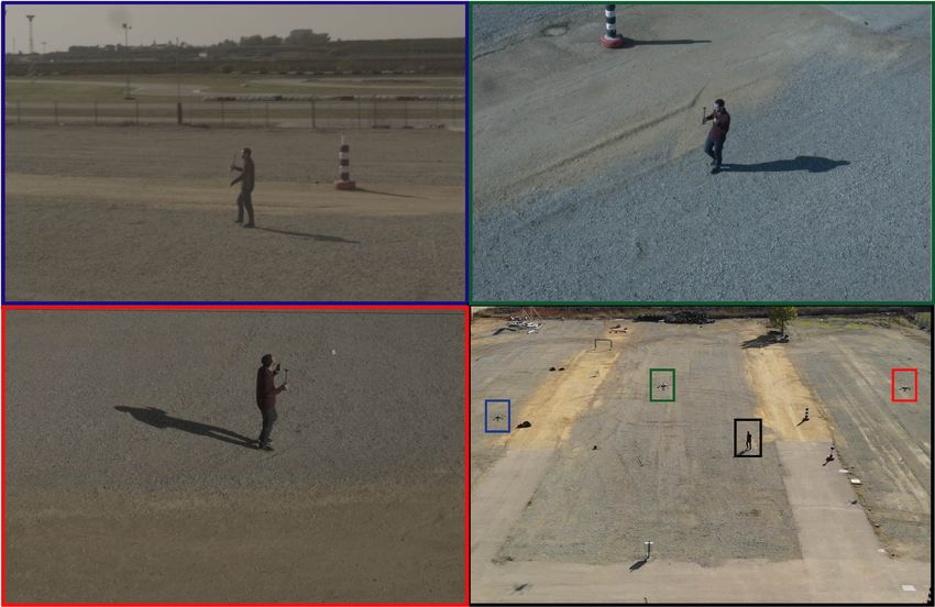
The cinematography UAVs used in our experiments were like
the one in Figure 9. They were custom-designed hexacopters
made of carbon fiber with a size of 1.80 × 1.80 × 0.70 m and had
the following equipment: a PixHawk 2 autopilot running PX4
for flight control; a RTK-GPS for precise localization; a 3-axis
gimbal controlled by a BaseCam (AlexMos) controller receiv-
ing angle rate commands; a Blackmagic Micro Cinema camera;
and an Intel NUC i7 computer to run our software for shot exe-
cution. The UAVs used Wi-Fi technology to share among them
their plans and communicate with our Ground Station. More-
over, as explained in Section 4, our target carried a GPS-based
device during the experiments, to provide positioning measures
to the Target Tracker component on board the UAVs. The de-
vice weighted around 400 grams and consisted of a RTK-GPS
receiver with a Pixhawk, a radio link and a small battery. This Figure 9: One of the UAVs used during the field experiments.
target provided 3D measurements with a delay below 100 ms,
that were filtered by the Kalman Filter on the Target Tracker to
achieve centimeter accuracy. These errors were compensated work Forces Pro [35] to generate a compiled library for the
by our gimbal controller to track the target on the image. non-linear optimization of our specific problem. The param-
We integrated the architecture described in Section 4 into our eters used for the algorithm in the experiments were also those
UAVs, using the ROS framework. We developed our method in Table 1. For collision avoidance, we used rcol = 5 m, a value
for trajectory planning (Section 3) in C++ 4 , using the frame- slightly increased for safety w.r.t. our simulations. All trajecto-
ries were computed on board the UAVs online at 0.5 Hz, with a
4 https://github.com/alfalcmar/optimal_navigation. receding horizon of N = 100 (10 s). Then, the Trajectory Fol-
111 2
3
3
Target
Figure 11: Example images from the cameras on board the UAVs during the
experiment: top left, UAV 1 (blue); top right, UAV 2 (green); and bottom left,
UAV 3 (red). Bottom right, a general view of the experiment with the three
UAVs and the target.
Traveled
UAV Acc (m/s2 ) Dist (m)
distance (m)
Figure 10: Trajectories followed by the UAVs and the human target during the
1 95 0.125 9.543
field experiment. UAV 1 (blue) does a lateral, UAV 2 (green) a flyby and UAV 2 141.4 0.108 9.543
3 (red) a lateral. 3 98.6 0.100 14.711
Table 4: Metrics of the trajectories followed by the UAVs during the field ex-
lower modules generated 3D velocity commands at 10 Hz to be periment. We measure the total traveled distance for each UAV, the average
sent to the UAL component, which is an open-source software norm of the 3D accelerations and the minimum distance (horizontally) to other
UAVs.
layer 5 developed by our lab to communicate with autopilot
controllers. Moreover, we assumed a constant speed model for
the target motion. This model was inaccurate, as the actual tar- itations and mutual visibility) and safety (i.e., inter-UAV colli-
get speed was unknown, but those uncertainties were addressed sion avoidance) constraints; and keeping the target on the cam-
by recomputing trajectories with the receding horizon. eras’ field of view, even under noisy target detections and un-
We designed a field experiment with 3 UAVs taking simul- certainties in its motion. Furthermore, we measured some met-
taneously different shots of a human target walking on the rics of the resulting trajectories (see Table 4) in order to eval-
ground. UAV 1 performs a lateral shot following the target side- uate the performance of our method. It can be seen that UAV
ways with a lateral distance of 20 m; UAV 2 performs a flyby accelerations were smooth in line with those produced in our
shot starting 15 m behind the target and finishing 15 m ahead in simulations and the minimum distances between UAVs were
the target motion line; and UAV 3 performs another lateral shot, always higher than the one imposed by the collision avoidance
but from the other side and with a lateral distance of 15 m. For constraint (5 m).
safety reasons, we established different altitudes for the UAVs,
3 m, 10 m and 7 m, respectively. In our decentralized trajectory
planning scheme, UAV 1 had the top priority, followed by UAV 7. Conclusions
2 and then UAV 3. Moreover, in order to design the shots of the
mission safely and with good aesthetic outputs, we created a re- In this paper, we presented a method for planning optimal
alistic simulation in Gazebo with all our components integrated trajectories with a team of UAVs in a cinematography applica-
and a Software-In-The-Loop approach for the UAVs (i.e., the tion. We proposed a novel formulation for non-linear trajectory
actual PX4 software of the autopilots was run in the simulator). optimization, executed in a decentralized and online fashion.
The full video of the field experiment can be found at https: Our method integrates UAV dynamics and collision avoidance,
//youtu.be/M71gYva-Z6M, and the actual trajectories fol- as well as cinematographic aspects such as gimbal limits and
lowed by the UAVs are depicted in Figure 10. Figure 11 shows mutual camera visibility. Our experimental results demonstrate
some example images captured by the onboard cameras during that our method can produce coordinated multi-UAV trajecto-
the experiment. The experiment demonstrates that our method ries that are smooth and reduce jerky movements. We also show
is able to generate online trajectories for the UAVs coping with that our method can be applied to different types of shots and
cinematographic (i.e., no jerky motion, gimbal mechanical lim- compute trajectories online for time horizons in the order of up
to 10 seconds, which seems enough for the considered cine-
matographic scenes outdoors. Moreover, our field experiments
5 https://github.com/grvcTeam/grvc-ual. proved the applicability of the method with an actual team of
12You can also read