PuppetMaster: Robotic Animation of Marionettes
←
→
Page content transcription
If your browser does not render page correctly, please read the page content below
PuppetMaster: Robotic Animation of Marionettes
SIMON ZIMMERMANN, ETH Zurich
ROI PORANNE, ETH Zurich and University of Haifa
JAMES M. BERN, ETH Zurich
STELIAN COROS, ETH Zurich
We present a computational framework for robotic animation of real-world
string puppets. Also known as marionettes, these articulated figures are
typically brought to life by human puppeteers. The puppeteer manipulates
rigid handles that are attached to the puppet from above via strings. The
motions of the marionette are therefore governed largely by gravity, the
pull forces exerted by the strings, and the internal forces arising from me-
chanical articulation constraints. This seemingly simple setup conceals a
very challenging and nuanced control problem, as marionettes are, in fact,
complex coupled pendulum systems. Despite this, in the hands of a master
puppeteer, marionette animation can be nothing short of mesmerizing. Our
goal is to enable autonomous robots to animate marionettes with a level of
skill that approaches that of human puppeteers. To this end, we devise a
predictive control model that accounts for the dynamics of the marionette
and kinematics of the robot puppeteer. The input to our system consists
of a string puppet design and a target motion, and our trajectory planning
algorithm computes robot control actions that lead to the marionette moving
as desired. We validate our methodology through a series of experiments
conducted on an array of marionette designs and target motions. These
experiments are performed both in simulation and using a physical robot,
the human-sized, dual arm ABB YuMi® IRB 14000.
CCS Concepts: • Theory of computation → Nonconvex optimization;
• Computing methodologies → Physical simulation; • Computer sys-
                                                                                                Fig. 1. A robot (ABB YuMi® IRB 14000) controlling a bird-shaped, string-
tems organization → Robotic control;
                                                                                                driven marionette. This type of puppet is notoriously difficult to animate.
Additional Key Words and Phrases: Computer graphics, robotics, puppeteer-                       Our control framework generates optimal motion trajectories for the robot
ing, sensitivity analysis                                                                       puppeteer such that the marionette performs a user-specified motion.
ACM Reference Format:
Simon Zimmermann, Roi Poranne, James M. Bern, and Stelian Coros. 2019.
PuppetMaster: Robotic Animation of Marionettes. ACM Trans. Graph. 38, 4,                        by a small number of cables, and the internal forces arising from
Article 103 (July 2019), 11 pages. https://doi.org/10.1145/3306346.3323003                      mechanical articulation constraints. As such, the map between the
                                                                                                actions of a puppeteer and the motions performed by the marionette
1    INTRODUCTION                                                                               is notoriously unintuitive, and mastering this unique art form takes
Marionettes are articulated, string-actuated puppets that have pro-                             unfaltering dedication and a great deal of practice.
vided a medium for animation in performance arts since Ancient                                     With the long term goal of endowing robots with human-level
Greece. In the hands of a skilled puppeteer, marionettes produce                                dexterity when it comes to manipulating complex physical systems,
motions that are incredibly expressive, fluid and compelling. How-                              we present PuppetMaster – a physics-based motion planning frame-
ever, their deceptively natural movements conceal the fact that                                 work for robotic animation of marionettes. As illustrated in Fig. 2,
marionettes are very challenging to control. Marionettes are under-                             the input to our computational puppeteering system consists of:
actuated, high-dimensional, highly non-linear coupled pendulum                                  1) a kinematic description of the robot puppeteer (i.e. the hierar-
systems. They are driven by gravity, the tension forces generated                               chical arrangement of actuators and rigid links); 2) the design of
Authors’ addresses: Simon Zimmermann, ETH Zurich; Roi Poranne, ETH Zurich and                   the marionette, which includes the articulated puppet itself, the
University of Haifa; James M. Bern, ETH Zurich; Stelian Coros, ETH Zurich.                      control handles that the robot will be manipulating, as well as the
                                                                                                strings that attach the puppet to the handles; and 3) a target motion
Permission to make digital or hard copies of all or part of this work for personal or
classroom use is granted without fee provided that copies are not made or distributed           that the marionette should aim to reproduce. Our core technical
for profit or commercial advantage and that copies bear this notice and the full citation       contribution is a novel trajectory optimization method built upon a
on the first page. Copyrights for components of this work owned by others than the
author(s) must be honored. Abstracting with credit is permitted. To copy otherwise, or
                                                                                                physics simulator using an implicit time-stepping scheme. To com-
republish, to post on servers or to redistribute to lists, requires prior specific permission   pute derivatives of the system’s forward dynamics, we show how
and/or a fee. Request permissions from permissions@acm.org.                                     to apply sensitivity analysis techniques to entire motion trajectories,
© 2019 Copyright held by the owner/author(s). Publication rights licensed to ACM.
0730-0301/2019/7-ART103 $15.00
                                                                                                as well as how to effectively exploit the specific sparsity structure
https://doi.org/10.1145/3306346.3323003                                                         imposed by the time domain. Our mathematical model forms the

                                                                                                         ACM Trans. Graph., Vol. 38, No. 4, Article 103. Publication date: July 2019.
103:2 •       Zimmermann, S. et al

basis of a general, unified framework that enables optimization                physically correct. However, in favor of optimization problems that
algorithms to concurrently reason about: the robot puppeteer’s                 are easier to solve, these constraints are often treated in a soft
workspace (i.e. the space of reachable configurations for its end              manner, resulting in animations where external fictitious forces are
effectors) and movements; the limited and indirect control provided            merely minimized [Barbič et al. 2009; Pan and Manocha 2018; Schulz
by string-based actuation setups; the dynamic motions generated                et al. 2014]. Given that we wish simulation results to carry over to the
by the puppet in response to the robot’s actions; and continuous               real world, we instead develop a trajectory optimization technique
design parameters such as the lengths of the strings and their points          that guarantees Newton’s second law of motion is always satisfied,
of attachment on the control handles. The output generated by our              even for intermediate results, up to unavoidable discretization errors
planning framework consists of optimal motion trajectories that are            introduced by numerical integration schemes.
specified in the configuration space of the robot puppeteer.                      Dexterous manipulation of complex physical systems is another
   To evaluate the efficacy of our robotic puppeteering framework,             topic of research in computer animation that is relevant to our work.
we designed a set of experiments of increasing complexity. These               In particular, the trajectory optimization formulation we introduce
experiments include different types of under-actuated dynamical                complements recent model-based [Bai et al. 2016; Clegg et al. 2015]
systems that we wish a robot to skillfully control, and a varied array         and learning-based [Clegg et al. 2018] techniques developed for ma-
of motion-based task specifications. To assess the degree to which             nipulation of cloth and clothing. Our technique leverages derivatives
simulation results carry over to the real world, we further fabricated         of the physics simulation which we use to compute a marionette’s
several physical prototypes that are puppeteered by an ABB YuMi –              motions. In this respect, we borrow concepts from recent differen-
a human-sized, dual-arm robot.                                                 tiable simulators for rigid bodies [Todorov 2014]. However, in our
                                                                               formulation, first and second derivatives are computed via sensi-
                                                                               tivity analysis, and they can be taken with respect to the robot’s
2    RELATED WORK
                                                                               actions, or with respect to continuous parameters that define the
The study of motion has been a core research topic in computer                 marionette’s design. First order Sensitivity analysis, in both its direct
graphics since the field’s very beginning. Nevertheless, animation             and adjoint form [McNamara et al. 2004], is often used to compute
predates computers by thousands of years: since ancient times, chil-           gradients for steady-state [Auzinger et al. 2018] or quasi-static prob-
dren and adults alike have been fascinated by physical systems                 lems that are governed by force equilibrium [Ly et al. 2018; Pérez
– mechanical automatons, animatronic figures, robotic creatures,               et al. 2017]. In this paper, we show how to extend this very useful
puppets and marionettes – that are designed to generate natural                optimization technique to second order, for trajectories computed
movements. In recent years, these types of physical animation de-              using forward dynamics simulations, and how to exploit the specific
vices have started to receive considerable attention from the com-             structure imposed by the time domain to increase the computational
puter graphics community. We have witnessed, for example, com-                 efficiency of the motion optimization process.
putational approaches to designing mechanical toys [Coros et al.                  For the history and engineering aspects of traditional marionette
2013; Song et al. 2017; Thomaszewski et al. 2014; Zhang et al. 2017],          design and manipulation, we refer the interested reader to [Chen
physical characters that produce motions by virtue of precisely con-           et al. 2004], and we note that the challenge of controlling marionette
trolled deformations [Bern et al. 2017; Gauge et al. 2014; Megaro              motions has been studied before. For example, sharing our vision,
et al. 2017; Skouras et al. 2013; Xu et al. 2018], robotic creatures           Murphey and his collaborators developed dynamic models tailored
that walk [Megaro et al. 2015; Schulz et al. 2017], fly [Du et al.             to marionettes [Johnson and Murphey 2007]. Building on the tech-
2016] or even roller blade [Geilinger et al. 2018], etc. Each of these         nique described in [Hauser 2002], they also formulated trajectory
application domains demands techniques that are tailored to the                optimization as unconstrained problems [Murphey and Johnson
unique challenges and characteristics of different types of physical           2011; Schultz and Murphey 2012]. This was achieved by defining a
systems. The problem that we tackle in this work, namely robotic               projection operator that takes a candidate, non-physical trajectory
manipulation of marionettes, is closest to the work of Skouras and             and finds a valid one. The operator is introduced in the optimization
colleagues [Skouras et al. 2013]. However, while they address the              problem as an objective, making constraints redundant. However,
problem of designing quasi-static movements, our goal is to gener-             computing the gradient of this new objective demands an optimiza-
ate highly dynamic motion trajectories for string-driven physical              tion problem to be solved. Our method on the other hand provides
systems using dexterous robots as puppeteers.                                  analytic expressions for both first and second derivatives. Further-
   In the early days of computer graphics, animation techniques                more, while previous work focuses largely on simple motions (e.g.
relied largely on interpolation of artist-prescribed key-frames. With          treating the marionette as a simple suspended mass [Murphey and
such an approach, the onus is on the animator to manually create               Johnson 2011]) or transferring the motions of a human puppeteer
the illusion that a character’s motions obey the laws of physics. The          onto a robot [Yamane et al. 2004], we demonstrate a diverse array
tedious and error-prone nature of this process led to the sub-field            of marionette motions that are generated automatically.
of physically based character animation, which has generated a                    It is also worth noting the connection between marionette ani-
rich body of research over the past three decades. Our work draws              mation and the transport of cable-suspended payloads using cranes
inspiration from techniques that formulate motion synthesis as                 [Zameroski et al. 2006] or helicopters [Bernard and Kondak 2009;
optimization problems [Cohen 1992; Witkin and Kass 1988]. In                   Bisgaard et al. 2009]. In this context, the main focus is the handling
these formulations, equations of motion based on Newton’s second               of oscillations in high speed, rest-to-rest motions. Trajectory opti-
law are incorporated as constraints, resulting in motions that look            mization approaches have been proposed to tackle this challenge, as

ACM Trans. Graph., Vol. 38, No. 4, Article 103. Publication date: July 2019.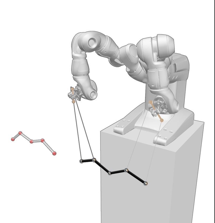
PuppetMaster: Robotic Animation of Marionettes • 103:3
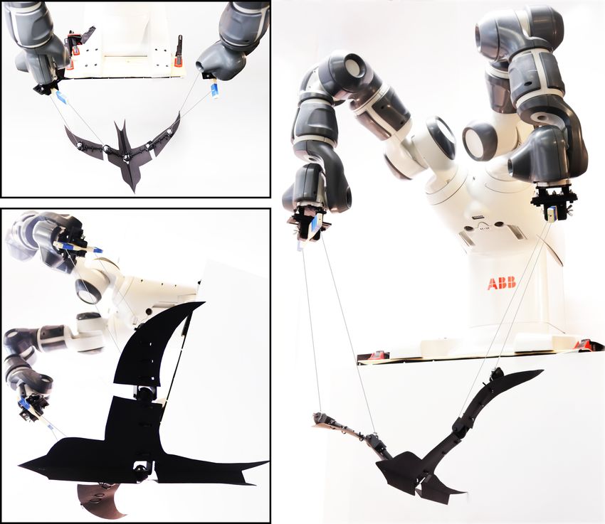
seen for example in [Sreenath et al. 2013] and [Sreenath and Kumar Robot puppeteer
2013], the latter of which focuses on collaborative transportation
via multi-drone systems. Methods based on reinforcement learning
have also been successfully developed [Crousaz et al. 2014; Faust
et al. 2013; Palunko et al. 2013], and they present an interesting q
Attachment
alternative to the model-based marionette control methodology we
points Handles
investigate in this paper.
3 OVERVIEW Target motion
ˆ
As illustrated in Fig. 2, our control framework takes as an input a
kinematic description of a robot puppeteer, the design of a string- s0
driven marionette, and a target motion. We visualize the marionette
as a virtual stick figure, and use two distinct visual styles, as seen
l0
in the figure, to portray the motion of the puppet, represented by a
vector x which encodes the trajectory for each point mass, and the
target motion x̂. Strings are used to attach the marionette to rigid
handles that are directly manipulated by the robot. We refer to the
points of attachment as p, and they control the pull forces applied Point mass
to the marionette through each string. The output of our system
consists of choreographed motions for the robot puppeteer, which Fig. 2. An overview of the main components of our system, which takes
as input a kinematic description of the robot puppeteer, a marionette de-
we encode using joint angle trajectories q. We refer the reader to
sign and a target motion. The output of our control framework consists of
the accompanying video for demonstrations and results.
precisely choreographed motions for the robot puppeteer.
We solve the robotic puppeteering control problem with a second-
order trajectory optimization method that exploits derivatives of
motions generated by forward dynamics simulation. These deriva- describe an inverse elastic shape design problem [Ly et al. 2018;
tives are computed using sensitivity analysis, as described in Section Megaro et al. 2017; Pérez et al. 2017]. First order sensitivity analysis
4. By exploiting the specific structure imposed by the time domain, has become a standard go-to technique for solving such problems,
we formulate a computationally-efficient trajectory optimization and it is therefore also suitable for our robotic marionette control
algorithm. In Section 5 we discuss the simulation model we use task. Briefly, sensitivity analysis provides an analytic expression
for our marionettes. Finally, in Section 6 we show experimental re- dx and it therefore enables the use of first order
for the Jacobian dp
sults, starting with simple systems such as a pendulum and a double gradient-based methods (e.g. L-BFGS) to minimize Eq. 2. To provide
pendulum, and ending with animal-inspired marionette designs. some intuition, for our problem setting, this Jacobian encodes the
way in which an entire motion trajectory x changes as a function of
4 PRELIMINARIES
the control actions p.
The control problem we seek to solve is characterized by two sets of
variables: state variables x, and control variables p, which represent First Order Sensitivity Analysis. Sensitivity analysis begins by
the motion trajectories of the marionette and of the robot, respec- applying the chain rule on O(x(p), p):
tively. The motion of the marionette is governed by the robot’s dO ∂O dx ∂O
actions and by its own non-linear dynamics. Without loss of gener- = + , (3)
dp ∂x dp ∂p
ality, we can therefore express x as an implicit function of p. While dx can be found
x(p) does not have a closed-form expression (we must compute it The analytic expression for the sensitivity term S := dp
through numerical simulation), the dependency between x and p is using the fact that G(x, p) is always zero (i.e. we assume that for any
captured by the relation p we can compute x(p) such that Eq. 1 is satisfied), which implies:
G(x, p) = 0, (1) dG ∂G ∂G
= S+ = 0. (4)
dp ∂x ∂p
which, as we will discuss shortly, encodes Newton’s second law of
motion for entire trajectories. Our control problem can therefore be By rearranging this equation, we get:
formulated as: ∂G −1 ∂G
min O(x(p), p), (2) S=− , (5)
p ∂x ∂p
where O(x(p), p) is an objective function that quantifies, for example, and plugging into (3), we obtain:
the degree to which the marionette’s motion matches its target, and dO ∂O ∂G −1 ∂G ∂O
the smoothness of the control actions. This problem formulation is =− + . (6)
dp ∂x ∂x ∂p ∂p
very generic. For example, if x was defined as the configuration of an
elastic object, p as the set of parameters that define its rest shape and We note that through a reordering of matrix multiplications, the
dx
well-known adjoint method [Cao et al. 2003] avoids computing dp
G(x, p) as the sum of internal and external forces, then Eq. 2 would
ACM Trans. Graph., Vol. 38, No. 4, Article 103. Publication date: July 2019.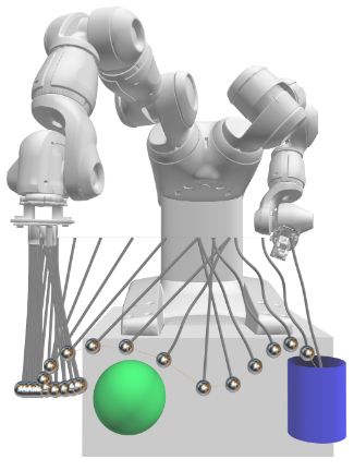
103:4 •       Zimmermann, S. et al

directly as it evaluates dO                                                                                                      Pendulum
                         dp . This is oftentimes more computationally                                   1.0
                                                                                                                       L-BFGS

                                                                                      Objective Value
                                                          dx to de-
efficient. However, as we will show next, we can leverage dp                                                           Gauss-Newton
rive a second-order, generalized Gauss-Newton solver that exhibits                                                     Newton
much better convergence properties than first order alternatives.

   Second Order Sensitivity Analysis. In our first experiments we
observed that first order optimization, i.e. L-BFGS, converges far too
                                                                                                 0             Iteration #         200 0          Time [s]     4
slowly. As an alternative, Newton’s method requires the Hessian
∂2 O , which can be derived using second order sensitivity analysis.                                                                 Bird
 ∂p2
                                                                                                        0.08

                                                                                      Objective Value
To begin with, we differentiate (3):
                                                                                                                      L-BFGS
               d2 O               d ∂O            d ∂O                                                                Gauss-Newton

                        d dO
                     =         =           S   +       .            (7)
               dp 2    dp dp     dp ∂x           dp ∂p
The formulas above involve third-order tensors, which lead to no-
tation that is slightly cumbersome. To simplify our exposition, we                                0            Iteration #           50 0         Times [s]        2
treat tensors as matrices and assume that contractions are clear
from context. For a conceptually similar but more formal derivation,                    Fig. 3. Comparison of the generalized Gauss-Newton approximation with
we refer the interested reader to [Jackson and Mccormick 1988].                         Newton and L-BFGS. The top row shows the number of iterations and
The second term in Eq. 7 is straightforward:                                            timings for one of the pendulum examples in Fig. 5. Newton’s method
                                                                                        occasionally stalls in non-convex regions, which largely contributes to the
                           d ∂O      ∂ 2O   ∂ 2O                                        less than satisfactory convergence. Its additional computational cost makes
                                = ST      +      ,                              (8)     it impractical for this problem. The bottom row shows the comparison for
                          dp ∂p      ∂x∂p ∂p2
                                                                                        the bird example in Fig. 8. In this case, Newton’s method takes an excessive
while the first term evaluates to                                                       amount of time and is not shown. In both cases it can be seen that the
                                                                                        generalized Gauss-Newton converges much faster. It is worth noting that
                d ∂O          d ∂O      ∂O d

                       S =           S+       S ,                               (9)     all intermediate results, whether or not the process converged, obey physics
               dp ∂x         dp ∂x      ∂x dp                                           becaues of the trajectory optimization strategy we employ.

with
                       d ∂O        ∂ 2O   ∂ 2O                                            Generalized Gauss-Newton. Although Newton’s method generally
                             = ST 2 +          .                               (10)     converges much faster than L-BFGS or gradient descent, there are
                      dp ∂x        ∂x     ∂x∂p
                                                                                        two issues with it. First, evaluating the second-order sensitivity term
       d S is a third-order tensor, and ∂O d S stands for

Here, dp                                ∂x dp
                                                                                        takes a non-negligible amount of time. Second, the Hessian is often
                                                                                        indefinite, and needs to be regularized. Both problems can be dealt
                        ∂O d        ∂O d2x i                                            with by simply excluding the tensor terms in (14). The result is a
                               Õ
                              S =              .                                        generalized Gauss-Newton approximation for the Hessian:
                        ∂x dp     i
                                    ∂x i dp2
                                                                                                                             ∂ 2O         ∂ 2O   ∂ 2O
                                   d S must be further broken down:                                                 H = ST        S + 2ST      +      .        (15)
The second-order sensitivity term dp                                                                                         ∂x 2         ∂x∂p ∂p2
                                                                                        Although H is not guaranteed to be positive-definite, we note that in
                                     ∂     ∂

                            d
                              S = ST    S+    S .                              (11)     our case, O is a convex function of x, and therefore the first term is
                           dp        ∂x    ∂p                                           always well-behaved. Furthermore, for our control problem, O does
The partial derivatives of S can be found by taking the second                          not explicitly couple x and p, and therefore the mixed derivative
derivatives in (4) and rearranging the terms. This results in                           (i.e. the second) term vanishes. The last term can be indefinite, but
                                                                                        we rarely encountered this case in practice.
                 ∂          ∂G −1 ∂ 2 G      ∂2 G

                    S=−                  S +        ,         (12)                         Sensitivity analysis for motion trajectories. The implicit relation-
                ∂x          ∂x      ∂x2      ∂p∂x                                       ship described by Eq. (1) is very general, and can easily be derived
                                                                                        for different types of dynamical systems and numerical integration
                    ∂        ∂G −1 ∂ 2 G    ∂2 G

                       S=−               S+        ,                           (13)     schemes. Here, we illustrate this process for mass spring systems,
                    ∂p       ∂x     ∂x∂p    ∂p2                                         since this is how we choose to model marionettes. In this context,
where once again we assume that the tensor expressions are self-                        the vector x has dimension 3nT , where n is the number of mass
evident. Combining all of the terms above leads to the following                        points, T is the number of time steps, and the constant 3 indicates
formula for the Hessian:                                                                that each mass point lives in a 3-dimensional space. We turn di-
                                                                                        rectly to the time-discretized setting and let xi , the i-th 3n block in
  d2 O   ∂O T ∂          ∂        T ∂ O        ∂ 2O     ∂ 2O
                                    2
                                                                                        x, denote the configuration of the system at time ti . As described

       =       S    S +    S   + S       S + 2        +      . (14)
  dp 2   ∂x      ∂x     ∂p          ∂x 2       ∂x∂p     ∂p2                             in [Martin et al. 2011], an Implicit Euler time stepping scheme is

ACM Trans. Graph., Vol. 38, No. 4, Article 103. Publication date: July 2019.
PuppetMaster: Robotic Animation of Marionettes • 103:5
−1
equivalent to finding xi that minimizes the functional ∂G ∂G
S = −
∂x
−1 ∂p
h2
Ui (xi ) = xÜ Ti MÜxi + W (xi , pi ) + gT xi , (16)
2
where xÜ i = ( xi −2xih−12 +xi −2 ) is the time-discretized acceleration, M = −
is the system’s mass matrix, h is the step size, W (xi , pi ) defines the
internal potential deformation energy stored in strings and trusses,
and the last term accounts for gravity; pi , similar to xi , encodes the
control actions taken at time step i. It is easy to verify that ∇xi Ui = 0
Fig. 4. The structure of the system can be used to compute S faster by block
(i.e. xi is a minimizer of Ui ) is equivalent to Newton’s second law, forward-substitution.
MÜxi = F(xi , pi ) where F(xi , pi ) = −∇xi W (xi , pi ), which means
that the equations of motion are satisfied.
Through Eq. 16, computing the motion of the marionette using
forward simulation is straightforward. We start from an input control We use a backtracking line search to find the step size α, where again,
trajectory p (the robot standing still is a valid choice for p), and x need to be recomputed for each test candidate p = p + αd in order
two fixed configurations, x0 and x−1 , which together represent the to evaluate O(x(p), p). We summarize the optimization procedure
starting state of the dynamical system. In order, from i = 1 to T , we in Algorithm 1. Note that in the next section we make a transition
then find xi that minimizes Ui using Newton’s method. from handle positions p to robot joint angles q, but the algorithm
In the context of forward dynamics, this standard numerical inte- essentially stays the same.
gration scheme also reveals the structure of the implicit relationship
described by Eq. (1). In particular, Gi , the i-th 3n block in G, is de-
Algorithm 1: Trajectory optimization
fined as ∇xi Ui . It is therefore clear that for any motion trajectory
computed through physics simulation, G(x, p) = 0, as required for Input: Dynamical system, initial p, initial x0 , xÛ 0 ,
sensitivity analysis. Output: Optimal control trajectory p
We discuss the specifics of our marionette model in the next sec-
tion, but we first highlight two important observations. First, it is while criterion not reached do
Compute x(p) using forward simulation
very easy to extend the concepts described above to different nu-
merical integration schemes. For example, the only change required Compute dO dp (Eq. (3))
to use BDF-2 (backward differentiation formula of second order), Compute H ((14) or (15))
which exhibits much less numerical damping than Implicit Euler, is Solve Hd = − dOdp
a different definition of the discretized acceleration. Second, upon Run backtracking line search in d
inspection, it is easy to see that the time domain imposes a very /* Simulate after every line search iteration */
specific structure on the system of equations that must be solved end
to compute the Jacobian dp dx in Eq. 4. This structure is visualized
in Fig. 4, and can be easily exploited to speed up computations. In
particular, since Gi depends explicitly only on xi , xi−1 , xi−2 and
pi (i.e. all other partial derivatives are 0), ∂G ∂p has a block diagonal
Relation to DDP. A well-known technique for optimal control is
∂G the Differential Dynamic Programming method (DDP). While New-
form, and ∂x has a banded block diagonal form. This allows us to ton’s method approximates the motion control objective through a
solve the resulting system using block forward-substitution, rather global quadratic function, DDP uses a sequence of local quadratic
than storing and solving the entire linear system represented by ∂G∂x . models derived for each individual time step. The resulting struc-
In our experiments, this results in a 5x speedup. We also note that ture gives rise to the characteristic backwards/forwards nature of
the resulting S is block triangular, which correctly indicates that xi DDP algorithms. Although both DDP and Newton’s method feature
does not depend on pj if j > i, or intuitively, the robot’s actions at quadratic convergence, the debate regarding which one performs
any moment in time only affect future motions of the marionette. best dates back to at least the 80s [Murray and Yakowitz 1984; Pan-
toja 1988] and continues today [Mizutani 2015]. Like Newton’s
Iterative optimization. Using either ddpO2 or its approximation H,
2
method, DDP and its Gauss-Newton approximation, the iterative
we can minimize (2) using a standard unconstrained optimization Linear Quadratic Regulator (iLQR), rely on a state transition func-
scheme, but we note one key difference: for each candidate p, we tion xi+1 = f (xi , pi ) and its first and second derivatives. In practice,
must always compute the corresponding x to ensure that (1) holds DDP and iLQR are typically applied in conjunction with explicit in-
before evaluating any of the derivatives. Once ∂O d2 O
∂p and H (or dp2 ) tegration schemes, because then f takes on an analytic form, and its
are computed, we find the search direction d by solving derivatives can be readily computed. Consequently, the techniques
we have described to compute derivatives of implicitly-integrated
dO forward dynamics simulations open up exciting opportunities for
Hd = − . (17)
dp DDP/iLQR optimal control formulations as well.
ACM Trans. Graph., Vol. 38, No. 4, Article 103. Publication date: July 2019.103:6 • Zimmermann, S. et al
5 ROBOTIC PUPPETEERING where s j01 j2 is the length of the string, k = 104 , and ψ (x) is a
5.1 The puppet model C 2 one-sided quadratic function modeling the unilateral nature
With the foundations for motion optimization laid out, we now of strings [Bern et al. 2017]:
describe the specifics of the simulation model we employ for mari- 1x2 + ϵ x + ϵ2 x≥0
2 2 6
onettes. Traditional marionettes are piece-wise rigid structures. In
ψ (x) = 1 x 3 + 1 x 2 + ϵ x + ϵ 2
0 > x > −ϵ (21)
our simulation model, we assume mass is concentrated at the joints.
6ϵ 2 2 6
0 otherwise
This matches the way we design and fabricate our physical proto-
types, which employ heavy steel balls as joint sockets, and much Here the constant ϵ = 1mm provides for a smooth transition be-
lighter 3D printed parts as structural frames (see the inset figure). tween the regime where the string is slack (and therefore applies
Furthermore, since we no force), and where it is taut and applies tension forces, which
are using fully implicit can pull but not push. First, second and third derivatives (the latter
integration schemes for required for Eq. 6) with respect to x and p are straightforward to
forward simulation, we compute analytically for both energy terms.
can model these struc-
tural frames as very stiff 5.2 Control
springs without worry-
We discussed our control optimization method in Section 4. Here
ing about stability prob-
we describe the different terms that define Eq. 2.
lems. A mass-spring representation of marionettes is therefore nat-
ural. This simple model has the additional benefit that it is uncon- Objectives. The main objective is, of course, to find a marionette
strained, and the mathematical formulation derived in the previous motion that is similar to the user specified trajectory x̂. To this end,
section needs only reason about positions, and not about rotations we define a simple quadratic objective that measures the similarity
as well. between the two:
The mass point representing each joint can optionally be con- O traj (x) = ∥x − x̂ ∥ 22 .
nected via strings to rigid control handles held by the robot. Impor-
We additionally regularize the acceleration of the string attachment
tant for our control problem is the world location of the attachment
j points to promote smooth motions, using the simple objective
point of string j at time index i. We denote this quantity by pi . Sim-
k
ilarly, we let xi represent the world position of the k-th mass point Ü 22 ,
O acc (p) = ∥p∥
at time index i. Its corresponding target location, which is provided where the acceleration vector pÜ is estimated using finite differences.
through the target animation, is represented by x̂ki . We assemble the Up to this point, the control problem operated directly in the space
positions of all mass points at time index i into a vector xi , and the of world trajectories for the string’s attachment points. However, we
positions of all string attachment points at time index i into a vector ultimately need to command the movements of the robot puppeteer,
pi . Finally, we assemble all xi into x, and all pi into p, forming the which will be specified as joint angle trajectories. These could be
state and control trajectories respectively. computed in post-processing using inverse kinematics (IK). The
To solve the equations of motion using Eq. (16), we formulate the pitfall of such a strategy is that it is quite likely that the motion
potential energy of the system as planner generates trajectories p which are not within the workspace
of the robot (i.e. they are not reachable), or they lead to inter-limb
W (xi , pi ) = Wpuppet (xi ) + Wstring (xi , pi ). (18) collisions. Following [Duenser et al. 2018], we eliminate this problem
with a simple extension that enables us to directly solve for control
The energy Wpuppet (xi ) measures the energy stored in the stiff
actions specified in the robot’s joint space.
springs we use to model a marionette’s body parts. Let L be the
set of pairs of joints connected by links. Then, Direct optimization of the robot’s motions. To compute trajectories
2 for the robot puppeteer’s joint angles, it suffices to express each
j j j j2 string attachment point pj as a kinematic function of the robot’s
Õ
Wpuppet (xi ) = k xi 1 − xi 2 − l 01 , (19)
{j 1, j 2 } ∈L joint angles q,
j
pi = FK(lj , qi ), (22)
j j
where k is a spring constant, and l 01 2 is the rest length defined by where FK is a standard forward kinematics function that computes
the marionette’s physical design. We use k = 104 for all our experi- the world coordinates of a point lj expressed in the local coordi-
ments, as we found this value sufficient to render the deformations nate frame of a robot’s gripper, and qi is a vector that stores the
of the robot’s body parts imperceptible. The energy Wstring (xi , pi ) robot’s joint angles at time index ti . With this definition in place,
measures the tension energy stored in the strings. Each string con- we can minimize the objective O(p(q)) directly as a function of q.
nects a marionette joint x j1 to an attachment point p j2 . We define the The changes introduced by this step are minimal – we only need to
set of joint-attachment point pairs by S, and define Wstring (xi , pi ) as apply the chain rule. For example, the gradient of the objective is
given by
j j j j2
Õ
Wstring (xi , pi ) = kψ xi 1 − pi 2 − s 01 , (20) dO dO dp ∂O
= + ,
(j 1, j 2 )∈S dq dp dq ∂q
ACM Trans. Graph., Vol. 38, No. 4, Article 103. Publication date: July 2019.PuppetMaster: Robotic Animation of Marionettes • 103:7
dp
where the Jacobian dq encodes how the world position of the attach-
ment points change with respect to the robot’s joint angles. This
Jacobian is straightforward to compute given the definition of the
forward kinematics map. The second derivative of the objective O
with respect to q can be computed in an analogous manner. Solving
directly for joint angle trajectories ensures that the optimization re-
sult is always feasible, and that it effectively exploits the workspace
of different types of robots. Furthermore, this formulation allows us
to define additional objectives to capture, for example, inter-limb
collisions or limits on joint angles and velocities. These objectives
take on standard forms, so we omit them here for brevity. We refer
the interested reader to [Duenser et al. 2018] for formal definitions.
Finding a convenient starting configuration. In simulation, we can Fig. 5. Interactive positioning of goals and obstacles. The user can reposition
set the marionette’s starting state (i.e. x0 and x−1 ) to any arbitrary the ball and the cup interactively, and the trajectory is updated in real-time.
values. However, when the robot starts to execute a performance, the See the accompanying video for more detail.
physical marionette must start from exactly the same configuration.
Consequently, x0 and x−1 should correspond to marionette poses
that are easily achievable. The only practical choice is to pick them (a) (b)
such that they represent a statically stable configuration given an
initial robot pose qinit . We find these configurations by setting
the simulated robot in the desired starting pose and then running
forward simulation until the system comes to rest.
6 EXPERIMENTAL RESULTS
In this section we summarize the results we generated with our
system. We begin with a few preliminary results and continue to
more elaborate examples that showcase our system’s capabilities.
Please refer to the accompanying video for a screen capture and
recording of the actual motions. We implemented our algorithm in
C++ using Eigen [Guennebaud et al. 2010], and ran it on a computer Fig. 6. Additional motions, also included in the accompanying video. Several
with an Intel Core i7-7709K 4.2Ghz. The average computation time robot poses are overlaid, and the trajectory of the point mass is approxi-
mately traced by a dashed line. (a) A double pendulum, which is known
for each forward simulation step (i.e. computing x(p)) as well as
for its chaotic behaviour, can still be accurately modeled for a short time
for computing the search direction d for each individual dynamical horizon. As in Fig. 5, we ask for a trajectory that avoids the obstacle, and
system can be found in Table 1. Acceptable control solutions begin reaches the cup. (b) In this case, the cup is fixed to the top of the handle
to emerge after a small number of iterations, and each intermediate and requires an agile motion to swing the point mass into the cup.
optimization result is valid due to the formulation we employ.
Interactive specification of goals. For small systems, our applica-
tion reacts at interactive rates. We began by testing a simple scenario model them with adequate accuracy. Finally, we ran an additional
involving a pendulum, where the goal is to place the suspended experiment where the cup was fixed to the top of the robot’s end
mass point inside a cup while avoiding a spherical obstacle. For this effector. Our optimization method successfully found a very agile
example, the robot’s end effector is constrained to move only along robot motion that swings the mass point just right so that it lands
a horizontal line through a dedicated control objective. The user can in the cup. This example also clearly shows the benefit of modeling
interactively position the cup and obstacle, and immediately observe strings as unilateral springs. We note that many of our other results,
the result. Fig 5 illustrates two examples that were obtained in this both in simulation and using physical prototypes, exploit the fact
manner. In one example the robot speeds towards the obstacle in that cables can go slack.
order to lift the weight above it, and then slows down to let it land in Puppet fabrication. We use heavy steel balls to fabricate ball-in-
the cup. In the second example, the robot first moves back and forth socket joints, and lightweight 3D printed frame structures for the
to gain momentum before swinging the weight above the obstacle. marionette’s bodies. The steel balls can be connected by strings to
This simple setting highlights the ability of our system to generate the control handles, and they are free to slide inside their sockets.
highly dynamic motions that are physically accurate. As shown in Fig. 7, hinge joints are also easy to model and fabricate.
We refer the reader to the accompanying video (and Fig. 6), where
we show a similar example, this time involving a double pendulum. Periodic motions. Periodic motions are very common in animation,
The dynamics of such systems are notorious for their chaotic be- and for marionettes in particular. We optimize for periodic motions
haviour, but for a reasonable planning horizon, we found we can still by adding an objective that minimizes the difference between the
ACM Trans. Graph., Vol. 38, No. 4, Article 103. Publication date: July 2019.103:8 • Zimmermann, S. et al
Naive design Optimized design
Fig. 9. Continuous design optimization for the Dragon puppet. With a naive
handle design, where both handles are linear, the robot cannot reproduce
the target motion to a satisfying degree. The design optimization procedure
suggests to use a triangular handle, which then results in a much more
faithful animation.
Fig. 7. Fabrication of a hinge joint. In simulation, these joint are represented
using a simple frame structure. The black sphere represents a mass point of
negligible weight, which functions to model the behaviour of a hinge joint.
Design optimization. Designing appropriate handles and picking
suitable string lengths is not an intuitive task, as these parameters
Init cycle Periodic motion shape the space of motions a marionette can perform. In some cases,
a quick trial-and-error search suffices to find reasonable parameter
values, but we found it very useful (and easy) to devise an automated
procedure instead. Since all of our objectives are smooth with respect
to design parameters, we can optimize for these as well, again using
sensitivity analysis. At a conceptual level, it suffices to replace p
Target motion by any design parameter in the derivation we presented in the
previous sections. We use this approach to optimize the locations
of the attachment points in local coordinates lj from Eq. 22, and
j j
the string lengths s 01 2 from Eq. (20). Fig. 9 shows a typical case,
where the motion trajectory generated with a sub-optimal handle
design cannot reproduce the target closely enough. After design
optimization, the resulting motion follows the target much more
Fig. 8. Designing a periodic motion for the Bird puppet. A periodic motion is closely. In this case, design optimization found that using a triangle-
normally very dynamic, and there are virtually no points where the puppet shaped handle performs better for this specific motion. This would
is at rest. However, we require all motions to start in a resting configuration. have been difficult to intuitively predict.
To avoid this issue, periodic motions start with an initialization cycle, where The design problem also involves discrete vari-
the robot brings the puppet from rest to a specific position and velocity ables: the decision regarding which point masses
within the periodic motion. It then switches to the target periodic motion should be stringed and to which attachment points
plays a crucial role in shaping the space of permissi-
ble motions. We explore various possibilities in Fig.
initial and final positions and velocities of all the components: pup-
10 for a simple design of a puppet’s leg. The target
pet joints and end effectors. Specifically, we extend the time horizon
motion appears in the inset. The figure shows dif-
by one sample at each end, x 0 and x t +1 , which are not played back,
ferent patterns of connectivity of the point masses. As can be seen,
and define the objective
the quality of the resulting motion is influenced by this discrete
O CycPos (x, p) = ∥x1 − xt +1 ∥ 2 + ∥x0 − xt ∥ 2 . design decision. We currently do not have a way of automatically
optimizing this aspect of the design, but we rely on the interactivity
As mentioned above, we start all of our motions at a rest pose.
of our system to let the designer experiment with different options.
Starting a periodic motion from a rest pose would mean that the
puppet should come to a rest after each cycle. We overcome this by Physical experiments. To investigate the consequences of mod-
running an initialization cycle before switching to the cyclic motion elling approximations and the corresponding sim-to-real gap, we
itself. Given a periodic motion, the user can pick a starting point recorded the motions of some of our physical marionettes using
on the period, and the system will find a motion that matches the an Optitrack motion capture system. Fig. 11 summarizes some of
position and velocity of the puppet at that point of the periodic our findings by reporting the mismatch between the simulation
motion. This is done using an objective for the final position and results and the recorded motions for the Chinese Dragon puppet.
velocity. We show an example for the Bird puppet in Fig. 8, where While the movements of the robot initially match the simulated
the user wished to create a flying motion. The entry point into the trajectories quite well, drift does accumulate over time. Depending
periodic motion is at its beginning, when the wings are at the very on the complexity of the underlying dynamical system, this drift
top. The velocity at this point is admittedly small, but not vanishing. can become problematic. For example, for the Puppy marionette,
We stress that every other entry point works as well. we have noticed that after about 10 motion cycles played in an
ACM Trans. Graph., Vol. 38, No. 4, Article 103. Publication date: July 2019.PuppetMaster: Robotic Animation of Marionettes • 103:9
(a) (b) (c)
(d) (e) (f ) Fig. 12. Several marionettes animated with our system. Please refer to the
accompanying video for motions performed both in simulation and using
physical prototypes.
7 CONCLUSION, LIMITATIONS AND FUTURE WORK
We presented a control framework for robotic animation of mar-
ionettes. As demonstrated through a variety of experiments, the
simulation-based motion optimization technique that we have de-
veloped provides a promising solution for this very challenging
Fig. 10. Comparisons of various stringing options. The choice of how to control problem. Nevertheless, our work represents only a first step
string a puppet, e.g. where to attach a string to and to which point masses, in endowing robots with human-level skill, and it highlights excit-
can have a great impact on the space of permissible motions. Note that the ing opportunities for future investigations. For example, there are
handle locations are omitted from this figure for simplicity. The color coding aspects of a marionette’s motion that we are currently not mod-
of the strings indicates attachment to the same handle.
eling: string collisions, play and friction in the mechanical joints,
deformations of the frame structure, forces generated by clothing
or other aesthetic layers, etc. Fortunately, as long as such charac-
1.0 Sim-vs-real: difference between predicted and captured motions teristics of the dynamical system can be adequately modeled in a
0.05
forward dynamics simulation, the control optimization step may
Y - Position [m]
x
0
remain unchanged. We believe this decoupling is very powerful, as
Position [m]
0.05 Averaged Error
it allows different modeling choices to be studied in isolation.
y
0
0.05
As there are still unmodeled aspects of a marionette’s dynamics,
Physical some mismatches between the results predicted in simulation and
z
Simulation
0.0 0
-0.8 X - Position [m] 1 0 Time [s] 11 the corresponding real-world motions are unavoidable. Empirically
we have noticed that the sensitivities of a marionette’s motions (i.e.
Fig. 11. Sim-vs-real comparison for the Chinese Dragon example. We how much they change due to an external perturbation) can depend
tracked the motions of four markers placed on the marionette using a quite strongly on the way in which it is designed. For now, the
motion capture system. The figure on the left shows the measured (in number of strings and assignment of attachment points to control
grey) and predicted (in red) trajectories in the x - y plane, starting with handles is kept fixed in our framework, but in the future we plan to
the initialization step and followed by 10 periodic cycles. The plots on the develop optimization techniques for such discrete design choices.
right show the position error between simulation predictions and physical We also currently play back the robot puppeteer’s movements in an
measurements averaged over the four markers along the x, y and z axes.
open-loop manner. Nevertheless, feedback mechanisms that are able
to gracefully recover from perturbations or drift that accumulate
over time are also very important and should be investigated. And
last but not least, we are very excited by the prospect of mathemati-
open-loop fashion, the motions of the physical prototype can get cally analyzing the stability of a marionette’s motions, and by the
out of sync and no longer resemble the desired bounding gait. To possibility of explicitly incorporating aspects of robust design and
overcome problems due to drift, feedback loops should be used to control in our trajectory optimization scheme.
stabilize the nominal trajectories computed through optimization. Our long term goal is to enable robots to manipulate various types
of complex physical systems – clothing, soft parcels in warehouses
Further results. In addition to the examples shown in the paper, or stores, flexible sheets and cables in hospitals or on construction
we show several more results in the accompanying video. The re- sites, plush toys or bedding in our homes, etc – as skillfully as
sults show a variety of marionette designs and animations: a fish humans do. We believe the technical framework we have set up for
swimming, a snake slithering, and a puppy bounding and trotting. robotic puppeteering will also prove useful in beginning to address
See Fig. 12 and Table 1 for more information on the puppets. this very important grand-challenge.
ACM Trans. Graph., Vol. 38, No. 4, Article 103. Publication date: July 2019.103:10 • Zimmermann, S. et al
Table 1. List of puppets discussed in the paper and video. We list the number of point masses, strings and attachments points, and the duration of the
trajectory. The number of time steps was 40 in all cases. We also provide information regarding the number of iterations applied until a reasonable match of
the target trajectory was reached, as well as the average time per iteration to compute the forward simulation step x(p) and the search direction d. The latter
includes the time required to compute the gradient and the hessian H as well as the solve of the linear system presented in Eq. 17. We note that our code was
not optimized for run time and improvements can be made in order to significantly decrease these numbers.
# point # attachment planning
Puppet # strings animation # iterations time x(p) time d
masses points horizon
Pendulum 1 1 1 preliminary 1.0s / 1.33s 10 0.0041s 0.0561s
Double Pendulum 2 2 1 preliminary 1.0s / 1.33s 10 0.0043s 0.0585s
Single Leg 3 2-4 2-4 preliminary 1.0s 11 0.0027s 0.1252s
Chinese Dragon 5 5 5 flying 1.0s 19 0.0069s 0.4464s
Swallow 5 4 4 flying 1.33s 55 0.0065s 0.3216s
Fish 11 7 7 swimming 1.0s 21 0.0220s 2.2532s
Snake 9 9 9 slithering 1.6s 27 0.0102s 2.5396s
Puppy 14 10 10 bounding 1.0s 37 0.0216s 4.6403s
Puppy 14 10 10 trotting 1.0s 25 0.0270s 4.7045s
REFERENCES Damien Gauge, Stelian Coros, Sandro Mani, and Bernhard Thomaszewski. 2014. In-
Thomas Auzinger, Wolfgang Heidrich, and Bernd Bickel. 2018. Computational design teractive Design of Modular Tensegrity Characters. In The Eurographics / ACM
of nanostructural color for additive manufacturing. ACM Trans. Graph. 37, 4 (2018), SIGGRAPH Symposium on Computer Animation, SCA 2014, Copenhagen, Denmark,
159:1–159:16. https://doi.org/10.1145/3197517.3201376 2014. 131–138. https://doi.org/10.2312/sca.20141131
Yunfei Bai, Wenhao Yu, and C. Karen Liu. 2016. Dexterous Manipulation of Cloth. Moritz Geilinger, Roi Poranne, Ruta Desai, Bernhard Thomaszewski, and Stelian Coros.
Comput. Graph. Forum 35, 2 (2016), 523–532. https://doi.org/10.1111/cgf.12852 2018. Skaterbots: Optimization-based Design and Motion Synthesis for Robotic Crea-
Jernej Barbič, Marco da Silva, and Jovan Popović. 2009. Deformable Object Animation tures with Legs and Wheels. In Proceedings of ACM SIGGRAPH, ACM Transactions
Using Reduced Optimal Control. ACM Trans. Graph. 28, 3, Article 53 (July 2009), on Graphics (TOG) (Ed.), Vol. 37. ACM.
9 pages. https://doi.org/10.1145/1531326.1531359 Gaël Guennebaud, Benoît Jacob, et al. 2010. Eigen v3. http://eigen.tuxfamily.org.
James M. Bern, Kai-Hung Chang, and Stelian Coros. 2017. Interactive design of animated John Hauser. 2002. A Projection Operator Approach To The Optimization Of Trajectory
plushies. ACM Trans. Graph. 36, 4 (2017), 80:1–80:11. https://doi.org/10.1145/3072959. Functionals. IFAC Proceedings Volumes 35, 1 (2002), 377 – 382. https://doi.org/10.
3073700 3182/20020721-6-ES-1901.00312 15th IFAC World Congress.
M. Bernard and K. Kondak. 2009. Generic slung load transportation system using small Richard H. Jackson and Garth P. Mccormick. 1988. Second-order Sensitivity Analysis
size helicopters. In 2009 IEEE International Conference on Robotics and Automation. in Factorable Programming: Theory and Applications. Math. Program. 41, 1-3 (May
3258–3264. https://doi.org/10.1109/ROBOT.2009.5152382 1988), 1–27. https://doi.org/10.1007/BF01580751
Morten Bisgaard, Jan Bendtsen, and Anders La Cour-Harbo. 2009. Modelling of Generic E. Johnson and T. D. Murphey. 2007. Dynamic Modeling and Motion Planning for
Slung Load System. In AIAA Modeling and Simulation Technologies Conference and Marionettes: Rigid Bodies Articulated by Massless Strings. In Proceedings 2007 IEEE
Exhibit. American Institute of Aeronautics and Astronautics. https://doi.org/10. International Conference on Robotics and Automation. 330–335. https://doi.org/10.
2514/6.2006-6816 1109/ROBOT.2007.363808
Yang Cao, Shengtai Li, Linda Petzold, and Radu Serban. 2003. Adjoint sensitivity analysis Mickaël Ly, Romain Casati, Florence Bertails-Descoubes, Mélina Skouras, and Laurence
for differential-algebraic equations: The adjoint DAE system and its numerical Boissieux. 2018. Inverse Elastic Shell Design with Contact and Friction. In SIGGRAPH
solution. SIAM Journal on Scientific Computing 24, 3 (2003), 1076–1089. Asia 2018 Technical Papers (SIGGRAPH Asia ’18). ACM, New York, NY, USA, Article
I.-Ming Chen, Raymond Tay, Shusong Xing, and Song Huat Yeo. 2004. Marionette: From 201, 16 pages. https://doi.org/10.1145/3272127.3275036
Traditional Manipulation to Robotic Manipulation. In International Symposium Sebastian Martin, Bernhard Thomaszewski, Eitan Grinspun, and Markus H. Gross.
on History of Machines and Mechanisms. Springer, Dordrecht, 119–133. https: 2011. Example-based elastic materials. ACM Trans. Graph. 30, 4 (2011), 72:1–72:8.
//doi.org/10.1007/1-4020-2204-2_10 https://doi.org/10.1145/2010324.1964967
Alexander Clegg, Jie Tan, Greg Turk, and C. Karen Liu. 2015. Animating human dressing. Antoine McNamara, Adrien Treuille, Zoran Popović, and Jos Stam. 2004. Fluid Control
ACM Trans. Graph. 34, 4 (2015), 116:1–116:9. https://doi.org/10.1145/2766986 Using the Adjoint Method. In ACM SIGGRAPH 2004 Papers (SIGGRAPH ’04). ACM,
Alexander Clegg, Wenhao Yu, Jie Tan, C. Karen Liu, and Greg Turk. 2018. Learning to New York, NY, USA, 449–456. https://doi.org/10.1145/1186562.1015744
dress: synthesizing human dressing motion via deep reinforcement learning. ACM Vittorio Megaro, Bernhard Thomaszewski, Maurizio Nitti, Otmar Hilliges, Markus H.
Trans. Graph. 37, 6 (2018), 179:1–179:10. https://doi.org/10.1145/3272127.3275048 Gross, and Stelian Coros. 2015. Interactive design of 3D-printable robotic crea-
Michael F. Cohen. 1992. Interactive Spacetime Control for Animation. SIGGRAPH tures. ACM Trans. Graph. 34, 6 (2015), 216:1–216:9. https://doi.org/10.1145/2816795.
Comput. Graph. 26, 2 (July 1992), 293–302. https://doi.org/10.1145/142920.134083 2818137
Stelian Coros, Bernhard Thomaszewski, Gioacchino Noris, Shinjiro Sueda, Moira For- Vittorio Megaro, Jonas Zehnder, Moritz Bächer, Stelian Coros, Markus H. Gross, and
berg, Robert W. Sumner, Wojciech Matusik, and Bernd Bickel. 2013. Computa- Bernhard Thomaszewski. 2017. A computational design tool for compliant mecha-
tional design of mechanical characters. ACM Trans. Graph. 32, 4 (2013), 83:1–83:12. nisms. ACM Trans. Graph. 36, 4 (2017), 82:1–82:12. https://doi.org/10.1145/3072959.
https://doi.org/10.1145/2461912.2461953 3073636
Cédric De Crousaz, Farbod Farshidian, and Jonas Buchli. 2014. Aggressive optimal E. Mizutani. 2015. On Pantoja’s problem allegedly showing a distinction between
control for agile flight with a slung load. In in IROS 2014 Workshop on Machine differential dynamic programming and stagewise Newton methods. Internat. J.
Learning in Planning and Control of Robot Motion. Control 88, 9 (2015), 1702–1711. https://doi.org/10.1080/00207179.2015.1013063
Tao Du, Adriana Schulz, Bo Zhu, Bernd Bickel, and Wojciech Matusik. 2016. Com- Todd D Murphey and E. Johnson. 2011. Control aesthetics in software architecture
putational multicopter design. ACM Trans. Graph. 35, 6 (2016), 227:1–227:10. for robotic marionettes. In American Control Conference (ACC), 2011. IEEE, IEEE,
http://dl.acm.org/citation.cfm?id=2982427 3825–3830.
Simon Duenser, James M. Bern, Roi Poranne, and Stelian Coros. 2018. Interactive D. M. Murray and S. J. Yakowitz. 1984. Differential dynamic programming and Newton’s
Robotic Manipulation of Elastic Objects. In 2018 IEEE/RSJ International Conference method for discrete optimal control problems. Journal of Optimization Theory and
on Intelligent Robots and Systems, IROS 2018, Madrid, Spain, October 1-5, 2018. 3476– Applications 43, 3 (01 Jul 1984), 395–414. https://doi.org/10.1007/BF00934463
3481. https://doi.org/10.1109/IROS.2018.8594291 I. Palunko, A. Faust, P. Cruz, L. Tapia, and R. Fierro. 2013. A reinforcement learning
A. Faust, I. Palunko, P. Cruz, R. Fierro, and L. Tapia. 2013. Learning swing-free tra- approach towards autonomous suspended load manipulation using aerial robots. In
jectories for UAVs with a suspended load. In 2013 IEEE International Conference on 2013 IEEE International Conference on Robotics and Automation. 4896–4901. https:
Robotics and Automation. 4902–4909. https://doi.org/10.1109/ICRA.2013.6631277 //doi.org/10.1109/ICRA.2013.6631276
ACM Trans. Graph., Vol. 38, No. 4, Article 103. Publication date: July 2019.PuppetMaster: Robotic Animation of Marionettes • 103:11
Zherong Pan and Dinesh Manocha. 2018. Active Animations of Reduced Deformable
Models with Environment Interactions. ACM Trans. Graph. 37, 3, Article 36 (Aug.
2018), 17 pages. https://doi.org/10.1145/3197565
J. F. A. De O. Pantoja. 1988. Differential dynamic programming and Newton’s method. In-
ternat. J. Control 47, 5 (1988), 1539–1553. https://doi.org/10.1080/00207178808906114
Jesús Pérez, Miguel A. Otaduy, and Bernhard Thomaszewski. 2017. Computational
design and automated fabrication of kirchhoff-plateau surfaces. ACM Trans. Graph.
36, 4 (2017), 62:1–62:12. https://doi.org/10.1145/3072959.3073695
J. Schultz and T. Murphey. 2012. Trajectory generation for underactuated control of a
suspended mass. In 2012 IEEE International Conference on Robotics and Automation.
123–129. https://doi.org/10.1109/ICRA.2012.6225032
Adriana Schulz, Cynthia R. Sung, Andrew Spielberg, Wei Zhao, Robin Cheng, Eitan
Grinspun, Daniela Rus, and Wojciech Matusik. 2017. Interactive robogami: An
end-to-end system for design of robots with ground locomotion. I. J. Robotics Res.
36, 10 (2017), 1131–1147. https://doi.org/10.1177/0278364917723465
Christian Schulz, Christoph von Tycowicz, Hans-Peter Seidel, and Klaus Hildebrandt.
2014. Animating Deformable Objects Using Sparse Spacetime Constraints. ACM
Trans. Graph. 33, 4, Article 109 (July 2014), 10 pages. https://doi.org/10.1145/2601097.
2601156
Mélina Skouras, Bernhard Thomaszewski, Stelian Coros, Bernd Bickel, and Markus H.
Gross. 2013. Computational design of actuated deformable characters. ACM Trans.
Graph. 32, 4 (2013), 82:1–82:10. https://doi.org/10.1145/2461912.2461979
Peng Song, Xiaofei Wang, Xiao Tang, Chi-Wing Fu, Hongfei Xu, Ligang Liu, and Niloy J.
Mitra. 2017. Computational design of wind-up toys. ACM Trans. Graph. 36, 6 (2017),
238:1–238:13. https://doi.org/10.1145/3130800.3130808
Koushil Sreenath and Vijay Kumar. 2013. Dynamics, Control and Planning for Coop-
erative Manipulation of Payloads Suspended by Cables from Multiple Quadrotor
Robots. https://doi.org/10.15607/RSS.2013.IX.011
K. Sreenath, N. Michael, and V. Kumar. 2013. Trajectory generation and control of
a quadrotor with a cable-suspended load - A differentially-flat hybrid system. In
2013 IEEE International Conference on Robotics and Automation. 4888–4895. https:
//doi.org/10.1109/ICRA.2013.6631275
Bernhard Thomaszewski, Stelian Coros, Damien Gauge, Vittorio Megaro, Eitan Grin-
spun, and Markus H. Gross. 2014. Computational design of linkage-based characters.
ACM Trans. Graph. 33, 4 (2014), 64:1–64:9. https://doi.org/10.1145/2601097.2601143
Emanuel Todorov. 2014. Convex and analytically-invertible dynamics with contacts
and constraints: Theory and implementation in MuJoCo. In 2014 IEEE International
Conference on Robotics and Automation, ICRA 2014, Hong Kong, China, May 31 - June
7, 2014. 6054–6061. https://doi.org/10.1109/ICRA.2014.6907751
Andrew Witkin and Michael Kass. 1988. Spacetime Constraints. SIGGRAPH Comput.
Graph. 22, 4 (June 1988), 159–168. https://doi.org/10.1145/378456.378507
Hongyi Xu, Espen Knoop, Stelian Coros, and Moritz Bächer. 2018. Bend-it: design and
fabrication of kinetic wire characters. ACM Trans. Graph. 37, 6 (2018), 239:1–239:15.
https://doi.org/10.1145/3272127.3275089
Katsu Yamane, Jessica K. Hodgins, and H. Benjamin Brown. 2004. Controlling a motor-
ized marionette with human motion capture data. International Journal of Humanoid
Robotics 01, 04 (Dec. 2004), 651–669. https://doi.org/10.1142/S0219843604000319
D. Zameroski, G. Starr, J. Wood, and R. Lumia. 2006. Swing-free trajectory generation
for dual cooperative manipulators using dynamic programming. In Proceedings
2006 IEEE International Conference on Robotics and Automation, 2006. ICRA 2006.
1997–2003. https://doi.org/10.1109/ROBOT.2006.1641998
Ran Zhang, Thomas Auzinger, Duygu Ceylan, Wilmot Li, and Bernd Bickel. 2017.
Functionality-aware retargeting of mechanisms to 3D shapes. ACM Trans. Graph.
36, 4 (2017), 81:1–81:13. https://doi.org/10.1145/3072959.3073710
ACM Trans. Graph., Vol. 38, No. 4, Article 103. Publication date: July 2019.You can also read